Enhancing Semi-Supervised Clustering: A Feature Projection Perspective Wei Tang
Hui Xiong
Shi Zhong
Jie Wu
Dept. of CSE Florida Atlantic Univ.
MSIS Dept. Rutgers University
Data Mining & Research Yahoo Inc.
Dept. of CSE Florida Atlantic Univ.
[email protected]
[email protected]
[email protected]
[email protected]
ABSTRACT Semi-supervised clustering employs limited supervision in the form of labeled instances or pairwise instance constraints to aid unsupervised clustering and often significantly improves the clustering performance. Despite the vast amount of expert knowledge spent on this problem, most existing work is not designed for handling high-dimensional sparse data. This paper thus fills this crucial void by developing a Semi-supervised Clustering method based on spheRical KmEans via fEature projectioN (SCREEN). Specifically, we formulate the problem of constraint-guided feature projection, which can be nicely integrated with semi-supervised clustering algorithms and has the ability to effectively reduce data dimension. Indeed, our experimental results on several real-world data sets show that the SCREEN method can effectively deal with high-dimensional data and provides an appealing clustering performance.
Categories and Subject Descriptors H.2.8 [Database Management]: Database Applications Data Mining; I.5.3 [Pattern Recognition]: Clustering
General Terms Algorithms, Experimentation
Keywords Semi-Supervised Clustering, Pairwise Instance Constraints, Feature Projection
1. INTRODUCTION Semi-supervised clustering, learning from a combination of labeled and unlabeled data, has recently become a topic of significant interest to data mining and machine learning communities. Indeed, in many application domains, additional information such as some labeled instances or pairwise instance constraints are available and can be used to aid the unsupervised clustering process [4, 5, 10, 25, 26].
Permission to make digital or hard copies of all or part of this work for personal or classroom use is granted without fee provided that copies are not made or distributed for profit or commercial advantage and that copies bear this notice and the full citation on the first page. To copy otherwise, to republish, to post on servers or to redistribute to lists, requires prior specific permission and/or a fee. KDD’07, August 12–15, 2007, San Jose, California, USA. Copyright 2007 ACM 978-1-59593-609-7/07/0008 ...$5.00.
Existing methods for semi-supervised clustering can be generally grouped into three categories. First, the constraintbased methods aim to guide the clustering process with pairwise instance constraints [25] or initialize cluster centroids by labeled instances [4]. Second, the distance-based methods employ metric learning techniques to get an adaptive distance measure used in the clustering process based on the given pairwise instance constraints [26]. Finally, the hybrid method proposed by Basu et al. [5] unifies the first two methods under a general probabilistic framework. However, most existing semi-supervised methods are not designed for handling high-dimensional data. It is wellknown that the traditional Euclidean notion of density is not meaningful in high-dimensional data sets [7]. Since most semi-supervised clustering techniques are based on proximity or density, they often have difficulties in dealing with high-dimensional data. Therefore, it is necessary to integrate feature reduction into the process of semi-supervised clustering. The key challenge is how we can incorporate supervision into dimensionality reduction such that the reduced data can still capture the available class information. To this end, we propose a Semi-supervised Clustering method based on spheRical K-mEans via fEature projectioN (SCREEN). Specifically, we first formulate the problem of constraint-guided feature projection and provide an analytical solution to the associated optimization problem. Then, we exploit this constraint-guided feature projection technique to reduce the dimensionality of the original dataset and use constrained spherical K-means algorithm on the low-dimensional projected data for clustering. In this paper, we consider supervision provided in the form of must-link and cannot-link constraints on pairs of instances. A must-link constraint means that the pair of instances involved must reside in the same cluster while a cannot-link constraint means that the pair of instances should always be placed in different groups. Indeed, the use of must-link and cannot-link constraints is a natural and practical choice, because the labeled instances may not be available and are harder to collect than pairwise constraints. For example, in the context of clustering GPS data for lanefinding [25] or grouping different actors in movie segmentation [3], the complete class information may not be available in these cases, but the pairwise instance constraints can be extracted automatically with minimal effort. Also, a user who is not a domain expert is more willing to provide an answer to whether two objects are similar/dissimilar more than to specify explicit labels. Moreover, pairwise instance constraints are more general than class labels in that we
can always generate equivalent pairwise instance constraints from labeled instances, but not vice versa. Finally, we have conducted experiments on some realworld datasets from different application domains. Our experimental results show that, for high-dimensional data, the SCREEN method can achieve better clustering performance than the state-of-the-art, semi-supervised clustering methods. In addition to this, we provide an analysis on the relative importance of must-link and cannot-link constraints. This analysis indicates that cannot-link constraints are much more important than must-link constraints in providing supervision for the clustering process. Overview. The remainder of this paper is organized as follows. In Section 2, we introduce the general framework of our proposed SCREEN algorithm. Section 3 discusses the experimental results on several real-world datasets. Related work on the existing methods of semi-supervised clustering is discussed in Section 4. Finally, in Section 5, we draw conclusions and make suggestions for future work. Table 1: Summary of notations. Symbols Description N number of instances in the original dataset K number of pre-specified clusters X = {xi }N set of N unlabeled instances 1 U = {µi }K set of K cluster centroids 1 CM L set of must-link constraints CCL set of cannot-link constraints Cd×m difference matrix formed by CCL Mm×m covariance matrix of Cd×m F = {Fl }k1 projection matrix calculated from Mm×m ξl corresponding eigen value of Fl β ratio between must-links and cannot-links
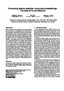
Figure 1 shows the framework of the SCREEN method. Given a set of instances and a set of supervision in the form of must-link constraints CM L = {(xi , xj )} where (xi , xj ) must reside in the same cluster, and cannot-link constraints CCL = {(xi , xj )} where (xi , xj ) should be in the different clusters, the SCREEN method is composed of three steps. In the first step, a pre-processing method is exploited to reduce the unlabelled instances and pairwise constraints according to the transitivity property of must-link constraints. In the second step, a constraint-guided feature projection method, called SCREENP ROJ , is used to project the original data into a low-dimensional space. Finally, we apply a version of semi-supervised clustering algorithms based on constrained spherical K-means on the projected low-dimensional dataset to produce the clustering results. The rest of this section is organized as follows. In Section 2.1, we introduce our initialization method for the unlabeled instances and pairwise constraints in detail. Section 2.2 presents the constraint-guided feature projection method– SCREENP ROJ –which gives an analytical solution to the optimization problem in finding the projection matrix. Finally, in Section 2.3, we describe our semi-supervised clustering based on constrained spherical K-means to produce the final clustering results. b5 b1 a2
Must−link Cannot−link
Must−link a
a3
b
b4
b w=5
a w=3
b2
a1
d
b3 Cannot−link
d w=1 Cannot−link
c1
c
c3 Must−link
c w=3
c2
Figure 2: An Illustration of Initialization.
2. THE SCREEN METHOD Before we describe the SCREEN method, we summarize the main notations used in this paper in Table 1.
Unlabeled Instances
Must−links Cannot−links
Preprocessing
Reduced Instances
Cannot−link Constraints
Feature Projection
Projected Instances
PC Spherical K−means
Cluster 1
Cluster 2
...
Cluster k
Figure 1: The Framework of the SCREEN Method.
2.1
Initialization
If there is no error in the pairwise constraints, it is easy to demonstrate that the must-link constraints represent an equivalence relation. This enables us to replace each transitive closure of must-link constraints with its average instance as demonstrated in Figure 2, where the solid line represents the must-link constraint and the dashed line represents the cannot-link constraint. In Figure 2, original instances are shown in white nodes and the average instances of transitive closures are represented by grey nodes. Sets {a1 , a2 , a3 }, {b1 , b2 , b3 , b4 , b5 }, and {c1 , c2 , c2 } represent different transitive closures forced by must-link constraints. After initialization, we can eliminate all must-link constraints and use the average instances a, b and c in each closure to represent the original cannot-link constraints. In the transformed dataset, the size of each transitive closure becomes the weight of the representative instance. Note that if there are some erroneous constraints, we need to identify and remove them in the initialization step. However dealing with the mis-specified constraints is out of the scope of this paper. The benefit of initialization is that we simplify the problem of constraint-guided clustering where we only need to focus on the cannot-link constraints in the optimization process as described in the following subsection. Another ben-
efit is that we can further reduce the size of unlabelled instances and cannot-link constraints. This is helpful for dealing with some large datasets.
2.2 SCREENP ROJ - A Constraint-Guided Feature Projection In the previous work [5, 26], the pairwise constraints were used for learning an adaptive metric between the prototype of instances. However, learning a distance metric among high-dimensional instances is very time consuming. More importantly, recent research on high-dimensional space has shown that the concept of distance in high-dimensional space may not be meaningful [7]. Instead of using constraintguided metric learning, in this paper we propose a constraintguided feature projection approach (SCREENP ROJ ) to further improve the performance of semi-supervised clustering in the high-dimensional datasets. The objective is to learn the projection matrix Fd×k = {F1 , . . . , Fk } containing k orthogonal unit-length d-dimensional vectors, which can project the original datasets into a low-dimensional space such that the distance between any pair of instances involved in the cannot-link constraints are maximized while the distance between any pair of instances involved in the must-link constraints are minimized. The objective function we try to maximize is: f=
X
kF T (x1 −x2 )k2 −
X
kF T (x1 −x2 )k2
(x1 ,x2 )∈CM L
(x1 ,x2 )∈CCL
(1) subject to the constraints FiT Fj
=
1 if i = j 0 if i 6= j
X
kw1 w2 · F T (x′1 − x′2 )k2
Theorem 1. Given the desired dimensionality k (k < d), ′ the set of cannot-link constraints CCL , and the covariance matrix M = cov(C) (where C is defined as above), the optimal projection matrix Fd×k is comprised of the first k eigenvectors of M corresponding to the k largest eigenvalues. Proof. Consider the objective function X kw1 w2 · F T (x′1 − x′2 )k2 f = ′ (x′1 ,x′2 )∈CCL
(3)
X
=
w12 w22
′ (x′1 ,x′2 )∈CCL
=
=
X
FlT (x′1 − x′2 )(x′1 − x′2 )T Fl
l
2
3
X
6 X 7 6 7 FlT 6 w12 w22 · (x′1 − x′2 )(x′1 − x′2 )T 7 Fl 4 ′ ′ 5
X
FlT (CC T )Fl =
l
l
(x1 ,x2 ) ′ ∈CCL
X
FlT M Fl
l
where Fl ’s are subject to constraints FlT Fh = 1 for l = h and 0 otherwise. Using the traditional Lagrange multiplier optimization technique, we write the Lagrangian LF1 ,...,Fk = f (F1 , . . . , Fk ) −
(2)
where k · k denotes L2 norm and F is the projection matrix whose column vectors are orthogonal to each other. As we described in Section 2.1, by applying the initialization methods shown in Figure 2, we can eliminate each transitive closure from must-link constraints with its equivalent average instance. Then, the objective function in Equation (1) can be further reduced to: f=
mal projection matrix F is given by the first k eigenvectors of the covariance matrix Md×d for a difference matrix Cd×m , where each column of C is a weighted difference vec′ tor w1 w2 · (x′1 − x′2 ) ∈ Rd for a pair (x′1 , x′2 ) in CCL and m is the number of pairs of cannot-link constraints.
k X
ξl (FlT Fl − 1) .
(5)
l=1
By taking the partial derivative of LF1 ,...,Fk with respect to each Fl and setting it to zero, we get ∂L = 2M Fl − 2ξl Fl = 0 ∀l = 1, . . . , k ∂Fl ⇒ M Fl = ξl Fl ∀l = 1, . . . , k .
(6)
It is clear from Equation (6) that solution Fl is an eigenvector of M and ξl is the corresponding eigenvalue of M. To maximize f , F must be the first k eigenvectors of M which makes f the sum of the k largest eigenvalues of M .
′ (x′1 ,x′2 )∈CCL ′
where {wi }N i=1 is the set of weights (which is measured by the number of instances in each transitive closure) for the reduced instances after pre-processing to the must-link constraints and N ′ is the reduced size of instances (N ′ ≤ N ). Note that in Equation (3), we still adopt the Euclidean distance instead of the cosine similarity as in the SPKM algorithm to calculate the objective value. This is because we work on the unit-length instances that satisfy the property in the following equation: kx − µk2 = kxk2 + kµk2 − 2xT µ = 2 − 2xT µ
(4)
From Equation (4), we can see that using the cosine similarity is equivalent to using the Euclidean distance when operating on the unit-length instances. There exists an analytical solution to the above optimization problem of finding the optimal projection matrix F in Equation (3). The following theorem shows that the opti-
After the constraint-guided feature projection as described above, we can represent the original instances in a lowdimensional space which conforms to the class information given in the form of pairwise constraints.
2.3
Constrained Spherical K-means
Since we eliminate the must-link constraints and shrink the original dataset in the initialization step, our version of constrained spherical K-means for semi-supervised clustering is slightly different from the one as shown in [25]. In this section, we introduce our version of constrained spherical K-means algorithm for semi-supervised clustering. Given a set of reduced instances X ′ = {x′1 , . . . , x′N ′ } with the corresponding weights W = {w1 , . . . , wN ′ }, a set of cannot-link constraints, and a pre-specified number of clusters K, we aim to find K disjoint partitions. As shown in [12], finding a feasible solution for the cannot-link constraints is much harder than that for the must-link constraints. It is computationally intractable to find an exact
Algorithm: SCREEN
cluster assignment which does not break any cannot-link constraints. Therefore, we adopt a local greedy heuristic to update cluster centroids as follows. Given each cannot-link constraint (x′i , x′j ) ∈ CCL , we find two different cluster centroids µx′i and µx′j such that
′
Input: Set of unit-length instances X ′ = {xi }N 1 , set ′ of corresponding weight W = {wi }N 1 , set of cannot-link constraints CCL = {(x′i , x′j )}, and number of clusters K. Output: K partitions of the instances.
wi ·
T x′ i µx′ i
+ wj ·
x′i
T x′ j µx′ j
(7)
Steps:
x′j
1. X ′ = SCREENP ROJ (X , W, CCL )
is maximized and assign and to these two different centroids to avoid violating the cannot-link constraint. Figure 3 shows the pseudo-code of our Pairwise Constrained Spherical K-means (PCSKM) clustering algorithm. Algorithm: The Pairwise Constrained Spherical K-means (PCSKM) Clustering Algorithm ′ Input: Set of unit-length instances X ′ = {x′i }N 1 , set of ′ corresponding weight W = {wi }N 1 , set of cannot-link constraints CCL = {(x′i , x′j )}, and number of clusters K. Output: K partitions of the instances. Steps: 1. Initialize the K unit-length cluster centroids {µh }K h=1 , set t ← 1 2. Repeat until convergence For i = 1 to m
2. Xk′ = PCSKM(X ′ , W, CCL ), where k = 1, . . . , K 3. post-process Xk′ to be in accordance with the original instances X
Figure 4: An Overview of the SCREEN Method.
3.1
1. Six UCI datasets: balance-scale, ionosphere, iris, soybean, vehicle, and wine. Those datasets have been used in learning a distance metric [26] and the work on the constrained feature projection via RCA [3]. We use these relatively low-dimensional datasets to demonstrate the performance of SCREENP ROJ , in comparison with other dimensionality reduction methods such as PCA and RCA.
(a) For each instance x′i which does not involve in any cannot-link constraint, find the closest centroid yn = arg maxk x′ T i µk ; (b) For each pair of instances (x′i , x′j ) involved in cannot-link constraint, find two different centroids µk and µk′ which maximize wi · x′ T i µk + wj · x ′ T µ ; ′ j k (c) For cluster k, let Xk′ P = {x′i |yi =P k}, the centroid is estimated as µk = x∈X ′ /k x∈X ′ k ; k
2. Six data sets: tr11, tr12, tr23, tr31, tr41, and tr45 from the TREC collection are used to compare the performance of SCREENP ROJ with PCA and RCA on highdimensional datasets. These datasets are available in the CLUTO toolkit [17].
k
3. t ← t + 1 ;
Figure 3: The Pairwise Constrained Spherical Kmeans Clustering Algorithm.
3. In order to evaluate the overall performance of our SCREEN method, we also compare it with the stateof-the-art, semi-supervised clustering algorithms including the constrained metric learning method [26] and the HMRF-Kmeans algorithm [4] on the nine datasets of the 20-Newsgroup corpus. The 20-Newsgroup data consists of approximately 20, 000 newsgroup articles collected evenly from 20 different Usenet newsgroups. Many of the newsgroups share similar topics and about 4.5% of the documents are cross-posted over different newsgroups making the class boundary rather fuzzy. We applied the same pre-processing steps as in [13], i.e., removed stop words, ignored file headers, subject line and selected the top 2000 words by mutual information. Specific details of the datasets are given in Table 2. The Bow [19] library is used in generating those datasets from the 20-Newsgroup corpus.
It is worth noting that our algorithm for semi-supervised clustering differs from the one used in [5] in that we do not consider the relative importance among cannot-link constraints, and we do not utilize pairwise constraints to supervise the cluster centroids initialization. However, these techniques can be easily incorporated into our algorithm. Finally, an overview of our SCREEN method is shown in Figure 4. Please note that since the pre-process step to the pairwise constraints will shrink the original dataset, we need to post-process the resultant K partitions (clusters) in order to be in accordance with the original dataset.
3. EXPERIMENTAL RESULTS In this section, we study the performance of the SCREEN method. Specifically, we demonstrate: (1) the effectiveness of constraint-guided feature projection, (2) the relative impact of Must-link and Cannot-link constraints on the performance of the SCREEN method, (3) the choice of reduced dimensionality, (4) the computational performance of the SCREEN method, and (5) the clustering performance of SCREEN, compared with several existing semi-supervised clustering algorithms.
The Experimental Setup
Experimental Datasets. Our experiments were performed on a couple of real-world datasets from different application domains. There are six UCI datasets 1 [20], six datasets derived from TREC collections 2 and nine datasets constructed from 20-Newsgroup [18]. The descriptions of these data sets are summarized as follows.
Evaluation Measures. In this paper, we use normalized mutual information (NMI) as the clustering validation measure. NMI, an external validation metric, estimates the quality of clustering with respect to the given true labels of 1 2
http://www.ics.uci.edu/∼mlearn/MLRepository.html http://trec.nist.gov
Table 2: Nine Datasets from the 20-Newsgroup Corpus. Dataset Newsgroup included Group doc. Tot. doc. Binary1,2,3 talk.politics.mideast, talk.politics.misc 250 500 Multi51,2,3 comp.graphics, rec.motorcycles, 100 500 rec.sports.baseball, sci.space, talk.politics.mideast alt.atheism, comp.sys.mac.hardware, misc.forsale, rec.autos, rec.sport.hockey, sci.crypt, sci.electronics, sci.med, sci.space, talk.politics.gun
Multi101,2,3
50
500
0.55
0.95
Normalized mutal information
0.4 0.35 0.3 0.25 0.2
0.1 10
20
30
40 50 60 70 Number of constraints
80
90
0.18 0.16
0.85
0.8
0.75
0.85 0.8 0.75 0.7
30
40 50 60 70 Number of constraints
80
90
0.7 10
100
Original PCA RCA SCREENPROJ
0.45
20
(c)
Ionosphere (N=351,C=2,D=34,d=5)
0.5 Normalized mutal information
0.9
(b)
20
0.55
Original PCA RCA SCREENPROJ
0.95
0.12 10
100
Balance-scale (N=625,C=3,D=4,d=2)
Normalized mutal information
0.2
Original PCA RCA SCREENPROJ
0.9
0.14
0.15
(a)
0.22
0.4 0.35 0.3 0.25 0.2 0.15
30
40 50 60 70 Number of constraints
80
90
100
Iris (N=150,C=3,D=4,d=2)
Original PCA RCA SCREEN
1.2 Normalized mutal information
Normalized mutal information
0.45
Original PCA RCA SCREENPROJ
0.24
Normalized mutal information
Original PCA RCA SCREENPROJ
0.5
1
PROJ
0.8
0.6
0.4
0.1
0.65
(d)
10
20 30 Number of constraints
40
50
Soybean (N=47,C=4,D=35,d=4)
0.05 10
(e)
100
0.2 10
Vehicle (N=846,C=4,D=18,d=5)
(f)
20
30
40 50 60 70 Number of constraints
80
90
20
30
40 50 60 70 Number of constraints
80
90
100
Wine (N=178,C=3,D=13,d=5)
Figure 5: The clustering performance on six UCI datasets with different numbers of constraints (N : size of dataset; C: number of clusters; D: dimensionality of original data; d: reduced dimensionality after projection).
the datasets [24]. If Zˆ is the random variable denoting the cluster assignments of the instances and Z is the random variable denoting the underlying class labels, then NMI is defined as ˆ Z) I(Z; NMI = (8) ˆ + H(Z))/2 (H(Z) ˆ Z) = H(Z) − H(Z|Z) ˆ is the mutual information where I(Z; between the random variables Zˆ and Z, H(Z) is the Shanˆ is the conditional entropy of non entropy of Z, and H(Z|Z) ˆ Z given Z [11]. The range of NMI values is 0 to 1. In general, the larger the NMI value is, the better the clustering quality is. NMI is better than other external clustering validation measures such as purity and entropy, since it does not necessarily increase when the number of clusters increases. Finally, we implemented the SCREEN algorithm in Matlab and conducted our experiments on a machine with 4 Intel Xeon 2.8 GHz CPUs and 2G main memory running under the GNU/Linux operating system. For each test dataset, we
repeated experiments for 20 trials. For the UCI datasets, we randomly generated 100 pairwise constraints in each trial. For the Trec datasets and data sets from the 20-Newsgroup collection, we randomly generated 500 pairwise constraints from half of the dataset, and tested the performance on the whole dataset. Also, the final result is the average of the results from the 20 trials.
3.2
The Effectiveness of SCREENP ROJ
In this section, we compare SCREENP ROJ with some existing dimensionality reduction methods such as PCA and RCA3 . In order to do a thorough comparison, we used both relatively low-dimensional datasets from the UCI repository and high-dimensional datasets from the Trec corpus. For the low-dimensional UCI datasets, we used the standard Kmeans algorithm as the baseline clustering algorithm. For 3 Thanks to the authors for providing their code on-line at http://www.cs.huji.ac.il/∼tomboy/code/RCA.zip for [3]
0.8
0.6 0.5 0.4 0.3
Original PCA PCA+RCA PCA+SCREENPROJ
0.2
20
30
40 50 60 70 Number of constraints
80
90
0.6 0.5 0.4 0.3 Original PCA PCA+RCA PCA+SCREEN
0.2 0.1
100
10
0.4 0.35 0.3 0.25 0.2
0.1
30
40 50 60 70 Number of constraints
80
90
100
0.05 10
0.7
0.5 0.4 0.3 Original PCA PCA+RCA PCA+SCREENPROJ 20
30
40 50 60 70 Number of constraints
(d) tr31
80
90
0.6 0.5 0.4 0.3
Original PCA PCA+RCA PCA+SCREENPROJ
0.2
100
Normalized mutal information
0.8
0.7 Normalized mutal information
0.8
0 10
30
0.1 10
20
30
40 50 60 70 Number of constraints
80
90
100
(c) tr23
0.6
0.1
20
(b) tr12
0.7
0.2
Original PCA PCA+RCA PCA+SCREENPROJ
0.15
PROJ
20
(a) tr11
Normalized mutal information
Normalized mutal information
Normalized mutal information
Normalized mutal information
0.45
0.7
0.7
0.1 10
0.5
0.8
40 50 60 70 Number of constraints
80
90
0.6 0.5 0.4 0.3
Original PCA PCA+RCA PCA+SCREENPROJ
0.2 0.1 10
100
20
30
(e) tr41
40 50 60 70 Number of constraints
80
90
100
(f) tr45
Figure 6: Clustering performance on 6 Trec datasets with different numbers of constraints. the high-dimensional Trec datasets, we chose the spherical K-means algorithm [14] instead. For six UCI datasets, Figure 5 shows the clustering performance of standard K-means applied to the original as well as projected data by different dimension reduction algorithms with different numbers of pairwise constraints. As can be seen, RCA performs well on low-dimensional data. Also, the performance of RCA significantly improves as the number of available constraints increases. However, we can also observe that the performance of RCA can be worse than that of PCA when there is a small number of constraints in the datasets such as Vehicle and Wine (we know that PCA is unsupervised and does not use any pairwise constraints). In contrast, the performance of SCREENP ROJ is always comparable to, or better than that of PCA. Finally, we observe that the performance of SCREENP ROJ is comparable to that of RCA on Soybean and Iris datasets. However, our experiments on six high-dimensional Trec data sets show that the performance of RCA heavily depends on the dimensionality of the original data. Also, it is computationally expensive to directly apply RCA to highdimensional datasets. Indeed, for data sets with extremely high dimensions, we need to first reduce their dimension to a lower level before applying the RCA method. Therefore, for the purpose of a fair comparison, we first used PCA to project the original data into a 100-dimensional space, and then applied the different algorithms to further reduce the dimensionality to 30. Figure 6 shows the results of this experiment on six Trec datasets. In the figure, we observe that SCREENP ROJ nearly always achieves the best performance on all six test datasets. In contrast, although we first reduce the dimension of six data sets to 100 using PCA, the performance of RCA is still the worst among all the algorithms. In other words, RCA may not be a good dimension reduction method for high-dimensional data.
3.3
Must-link vs. Cannot-link
Here, we compare the relative impact of must-link and cannot-link constraints on the performance of the SCREEN method. In this experiment, we incorporate a parameter β to the objective function in Equation (3) to adjust the relative impact between must-link and cannot-link constraints: f
=
X
(1 − β) ·
kF T (x1 − x2 )k2
(x1 ,x2 )∈CCL
−β ·
X
kF T (x1 − x2 )k2
(9)
(x1 ,x2 )∈CM L
From Equation (9), we observe that β = 0 is equivalent to only using cannot-link constraints in finding the optimal feature projection matrix. When β = 1, we only use mustlink constraints to perform the feature projection. In our experiments, we varied the value of β in steps of 0.1 from 0 to 1. The clustering results, as measured by NMI, are plotted in Figure 7 with respect to different values of β. In the figure, the x-axis denotes the different values of parameter β and the y-axis denotes the clustering performance measured by NMI. As can be seen in Figure 7, there is no significant difference on the clustering performance when β is in the range of 0.1 to 0.9. However, when using only must-link constraints (β = 1) the clustering performance deteriorates sharply. This indicates that the cannot-link constraints are more important than the must-link constraints in guiding the feature projection to get meaningful representation for each instance in the low-dimensional space.
3.4
The Choice of Dimension k In this section, we empirically evaluate the impact of different number of reduced dimension k on the performance of
3.5
Normalized Mutual Information
0.9
Binary
1
0.8
Binary2
0.7
Binary3
0.6
Multi51
0.5
Multi5
Multi52 3
Multi101
0.4
Multi10
2
0.3
Multi103
0.2 0.1 0 0.1 0.3 0.5 0.7 0.9 Ratio between must−link and cannot−link constraints (Beta)
Figure 7: The relative impact of must-link and cannot-link constraints.
In the following two subsections, we evaluate the overall computational and clustering performance of our SCREEN method. The benchmark algorithms are listed as follows. • SPKM: the standard spherical K-means algorithm [14] which does not use pairwise constraints. It is worth noting that the method proposed in this paper is tailored for high-dimensional sparse data with directional characteristics, which mainly stem from text documents represented by the vector space model (VSM) [6]. The most relevant work in this application domain is SPKM, which adapts the standard K-means algorithm to cluster the normalized unit-length instances by using the cosine similarity as the proximity function. Hence, we chose SPKM as the baseline; • PCSKM: the pairwise constrained spherical K-means algorithm described in Figure 3, which can be regarded as another implementation of semi-supervised, constrained K-means described in [25];
80 70
Dimensionality k
Computational Performance
• PCSKM+M: the pairwise constrained spherical K-means algorithm preceded by an additional metric learning to get an adaptive distance between instances, which is proposed by Xing et al. [26];
60 50 40
• MPCSKM: the HMRF-Kmeans algorithm proposed by Basu et al [5]. This algorithm unifies the metric learning and constrained clustering into a general probabilistic framework4 .
30 20 10 Binary
Multi5
Multi10
Trec
Figure 8: The Choice of Reduced Dimension k.
the SCREEN method. Specifically, we test the performance of SCREEN in terms of NMI with respect to different values of k varing from 10 to 100. Given a specified k, we repeat experiments 20 times. In each trial, we randomly generate 250 pairwise constraints as additional information. The experimental results on the datasets from 20-Newsgroup and Trec collections are shown in Figure 8 as four boxplots, which corresponds to the experimental results on sub-datasets from Binary, Multi5, Multi10, and Trec. There are three sub-datasets: Binary1 , Binary2 , and Binary3 from the Binary data collection. The Binary boxplot shows the k values when SCREEN achieves the best clustering performance on these three sub-datasets. Also, the M ulti5 boxplot shows the k values when SCREEN has the best clustering performance on three sub-datasets: M ulti51 , M ulti52 , M ulti53 . In addition, the M ulti10 boxplot presents the k values for the case that SCREEN has the best clustering performance on three sub-datasets: M ulti101 , M ulti102 , M ulti103 . Finally, there are six sub-datasets: tr11, tr12, tr23, tr31, tr41, and tr45 from the Trec corpus. The T rec boxplots shows six k values which lead to the best clustering performance of SCREEN on these datasets. In Figure 8, we observe that SCREEN achieves the best performance at different k values for different datasets. However, we notice that the clustering performance is maximized when the median of k values is between k = 20 and k = 40. In all our experiments, we use this as a guideline for the choice of k values.
First, we evaluate the computational performance of the semi-supervised clustering algorithms on the selected 20Newsgroup datasets with respect to different numbers of pairwise constraints. Due to the space limit, for each category of the datasets we only give out one result since the datasets from the same category usually lead to similar outputs. The experimental results are summarized in Figure 9, where the x-axis denotes the number of pairwise constraints and the y-axis denotes the elapsed running time in log scale. Please note that since the MPCSKM algorithm is not implemented in Matlab, we did not include this algorithm for this comparison. As demonstrated in Figure 9, the execution time of SPKM is consistently the lowest among all the methods since it does not perform extra work in addition to enforcing the clustering process based on the pairwise constraints. The PCSKM+M algorithm via metric learning method is always the slowest when compared to other methods. This is because the metric learning method has to learn a different weight for each individual dimension. When the dimensionality is very high, the cost of metric learning will be very high compared to the constraint-guided feature projection. In Figure 9, we can see that the SCREEN method, which utilizes the feature projection method, is only slightly slower than the PCSKM algorithm due to the extra work on the supervised dimensionality reduction, but much faster than that of PCSKM+M algorithm. This is because it only involves an eigen value decomposition of a covariance matrix formed by cannot-link constraints, which can be implemented efficiently by Singular Value Decomposition (SVD). In addition, one can still explore some iterative methods, such as 4 Thanks to the authors for putting their implementation on-line at http://www.cs.utexas.edu/users/ml/risc/ for [5].
4
4
10 SPKM PCSKM PCSKM+M SCREEN
3
10 Execution time (secs)
10 Execution time (secs)
4
10 SPKM PCSKM PCSKM+M SCREEN
3
2
10
1
10
0
10
2
10
1
10
0
−2
10
50
150
200 250 300 350 Number of constraints
400
450
500
10
1
10
10
−1
100
2
10
0
10
−1
10
SPKM PCSKM PCSKM+M SCREEN
3
10 Execution time (secs)
10
50
−1
100
150
(a) Binary1
200 250 300 350 Number of constraints
400
450
500
10
50
100
(b) M ulti51
150
200 250 300 350 Number of constraints
400
450
500
(c) M ulti101
Figure 9: A Comparison of Computational performance using 20-Newsgroup datasets.
0.6 0.5 0.4 0.3
0.6 0.5 0.4 0.3 0.2
0.2 0.1 50
0.7
100
150
200 250 300 350 Number of constraints
400
450
0.1 50
500
150
Normalized mutal information
Normalized mutal information
0.5 0.4 0.3
0.8
400
450
0.5 0.4 0.3
0.1 50
500
0.9
0.6 0.5 0.4
150
200 250 300 350 Number of constraints
400
450
500
0.2 50
0.8
100
150
200 250 300 350 Number of constraints
400
450
Normalized mutal information
0.3
50
0.3
0.1 50
100
150
200 250 300 350 Number of constraints
(g) M ulti101
100
400
450
500
150
200 250 300 350 Number of constraints
450
500
SPKM PCSKM PCSKM+M SCREEN MPCSKM
0.7
0.4
0.1 50
400
0.5
(f) M ulti53
0.5
0.2
500
0.8
0.6
0.2
450
0.6
500
SPKM PCSKM PCSKM+M SCREEN MPCSKM
0.7
0.4
400
0.7
0.8
0.5
200 250 300 350 Number of constraints
SPKM PCSKM PCSKM+M SCREEN MPCSKM
(e) M ulti52
SPKM PCSKM PCSKM+M SCREEN MPCSKM
150
0.4
0.3
100
100
(c) Binary3
0.7
0.8
Normalized mutal information
0.6
1
(d) M ulti51
0.6
200 250 300 350 Number of constraints
SPKM PCSKM PCSKM+M SCREEN MPCSKM
0.9
0.6
0.7
0.7
1 SPKM PCSKM PCSKM+M SCREEN MPCSKM
0.7
0.2 50
0.8
SPKM PCSKM PCSKM+M SCREEN MPCSKM
(b) Binary2
1
0.8
0.9
0.2 100
(a) Binary1
0.9
1 Normalized mutal information
0.7
SPKM PCSKM PCSKM+M SCREEN MPCSKM
Normalized mutal information
0.8
0.8
Normalized mutal information
0.9
0.9
SPKM PCSKM PCSKM+M SCREEN MPCSKM
Normalized mutal information
Normalized mutal information
1
0.6 0.5 0.4 0.3 0.2 0.1
100
150
200 250 300 350 Number of constraints
(h) M ulti102
400
450
500
0
50
100 150 Number of constraints
200
250
(i) M ulti103
Figure 10: A Comparison of Clustering performance using 20-Newsgroup datasets. EM algorithm for PCA [23] or Nystrom method [9], to further improve the efficiency.
3.6 A Comparison of Clustering Performance Here, we compare the clustering performance of various semi-supervised clustering algorithms. The results are shown in Figure 10, where the x-axis denotes the number of pairwise constraints, and the y-axis denotes the clustering per-
formance in terms of NMI. We have tested various values of k - the number of reduced dimension. Due to the space limit, we select k = 30 to report the results. In general, it is clear that on most datasets, the clustering performance of all algorithms constantly improve with the increase of the number of pairwise constraints. However, the clustering performance of the SCREEN method is more stable compared to the other methods, and always
outperforms the PCSKM+M algorithm via metric learning and MPCSKM algorithm via HMRF model. This is mainly due to the fact that constraint-guided feature projection can easily produce more condensed and meaningful representations for each instance. In addition, PCSKM+M is not much better than the PCSKM algorithm except for the Multi10 dataset. This is because it is a big challenge for metric learning to learn a reasonable distance measure between any pair of sparse instances in the original high-dimensional space.
4. RELATED WORK The related literature on semi-supervised clustering can be grouped into three categories: constraint-based methods, distance-based methods, and a combination of constraintbased and distance-based methods. For constraint-based methods, the cop-kmeans algorithm [25] guides the cluster allocation process by a constraint motivated heuristic objective function. However, this algorithm strictly enforces the clustering process such that any violation of the given pairwise constraints is forbidden, which limits its use, especially in a noisy environment. In contrast, our version of semi-supervised clustering algorithm allows some relaxation of the pairwise constraints. Also, Basu et al. [4] proposed a seeded K-means which tries to get better initial cluster centroids from the labeled instances in addition to constraining the clustering process, while their supervised cluster initialization is based on the labeled instances instead of pairwise constraints. For distance-based methods, Cohn et al. [10] used gradient descent for weighted Jensen-Shannon divergence in the context of EM clustering. Xing et al. [26] combined the Newton Raphson method and iterative projection together to learn a Mahalanobis distance for K-means clustering. De Bie et al. [8] proposed a more efficient algorithm for learning the distance metric with side information, which utilized Canonical Correlation Analysis (CCA) to approximate LDA. In general, the metric learning used in the distancebased method, which is equivalent to learning an adaptive weight for each dimension, is either based on iterative algorithms, such as gradient descent and Newton’s method, or involves some matrix operations. However, the distancebased method has high computational cost when applied to the high-dimensional data. Indeed, data represented in matrix is often singular when the sparsity of the data is high. This makes some matrix operations, such as inversion, computationally intractable. For hybrid methods, Basu et al. [5] introduced a general probabilistic framework which unifies the constraint-based and distance-based method into the Hidden Markov Random Field (HMRF). The proposed HMRF-EM algorithm can interweave the constrained clustering and distance learning interactively in the process of semi-supervised clustering. Also, the related literature on feature reduction includes Principle Component Analysis (PCA) [22] which tries to find a low rank approximation to represent the high-dimensional data, and Fisher’s Linear Discriminant Analysis (LDA) [15] which tries to find one or more directions along which different classes can be best separated while the variance of each class is minimized given the label for each instance. The PCA method works in an unsupervised manner where the class information is not available, which makes the reduced dataset incapable of capturing the original class information. In contrast, the LDA method needs to know the exact
information in order to calculate the between/within-class scatter matrix. Our constraint-guided feature projection method differs from the traditional LDA method in that we incorporate a more general supervision in the form of pairwise constraints instead of the complete class information which may be unavailable in certain application domains. To the best of our knowledge, the most related work is the Relevant Component Analysis (RCA) algorithm [3], which is based only on must-link constraints and tries to learn a Mahalanobis distance using Whitening transform [16]. In this paper, our major focus is to provide an alternative way to improve the semi-supervised clustering for high-dimensional sparse data by constraint-guided feature projection instead of metric learning. Existing approaches for clustering high-dimensional data usually involve the use of feature projection and feature selection. Feature projection techniques, as we described above, attempt to represent a dataset by its latent variables which are usually much fewer than the number of original features. Feature selection methods select only the most relevant dimensions from a dataset to summarize its instances. The typical algorithms of feature selection include “wrapper methods” and “filter methods”. The recently proposed subspace clustering algorithm [21] can be regarded as an extension to the feature selection methods which attempts to find clusters in different subspaces of the same datasets. Existing subspace clustering algorithm can be grouped into two categories: the top-down method such as projected clustering [1] and the bottom-up method such as CLIQUE [2] etc. An excellent survey on techniques of subspace clustering is available in [21]. It is worth noting that the recently proposed method on semi-supervised projected clustering [27] utilized the limited supervision in the form of labeled instance in subspace clustering. The motivation of this work is to find a more compact representation for each cluster to efficiently represent the instances within it. Also, they used feature selection instead of feature projection in applying the supervision in each cluster. This is different from our method.
5.
CONCLUSIONS AND FUTURE WORK
In this paper, we proposed a Semi-supervised Clustering method based on spheRical K-mEans via fEature projectioN (SCREEN), which is tailored for handling sparse, highdimensional, data. Specifically, the SCREEN method first uses the constraint-guided feature projection to reduce the dimensionality and then applies the constrained spherical K-means algorithm to cluster data with reduced dimension. In the development of the SRCEEN method, we formulate the problem of constraint-guided feature projection as an optimization problem. The goal is to find a feature projection matrix based on the pairwise instance constraints, and give an analytical solution which can be implemented without too much effort. In addition, for the constrained spherical K-means algorithm, we introduce a heuristic solution to loosely enforce the pairwise constraints, which enable it to be applied in much wider application domains. Finally, we have compared the SCREEN method with existing semi-supervised clustering methods using real-world datasets. The experimental results indicate that SCREEN can achieve a better clustering performance with a smaller computational cost. We also studied the relative impact of must-link and cannot-link constraints in guiding the clustering process. Our analysis shows that the cannot-link con-
straints are more important than the must-link constraints in providing meaningful class information. There are several potential directions for future research. First, we are interested in automatically identifying the right number for the reduced dimensionality based on the background knowledge other than providing a pre-specified value. Second, we plan to explore alternative methods to employ supervision in guiding the unsupervised clustering, e.g., supervised feature clustering.
6. ACKNOWLEDGMENTS We thank Dr. Xingquan Zhu at Florida Atlantic University for his insightful comments. This research was supported in part by an IBM Faculty Award, by a Faculty Research Grant from Rutgers Business School-Newark and New Brunswick, and by a Motorola Research Grant.
7. REFERENCES [1] C. C. Aggarwal, C. M. Procopiuc, J. L. Wolf, P. S. Yu, and J. S. Park. Fast algorithms for projected clustering. In Proc. of the ACM SIGMOD International Conference on Management of Data (SIGMOD-99), pages 61–72, 1999. [2] R. Agrawal, J. Gehrke, D. Gunopulos, and P. Raghavan. Automatic subspace clustering of high dimensional data for data mining applications. In Proc. of the ACM SIGMOD International Conference on Management of Data (SIGMOD-98), pages 94–105, 1998. [3] A. Bar-Hillel, T. Hertz, N. Shental, and D. Weinshall. Learning distance functions using equivalence relations. In Proc. of the 20th International Conference on Machine Learning (ICML-03), pages 11–18, 2003. [4] S. Basu, A. Banerjee, and R. J. Mooney. Semi-supervised clustering by seeding. In Proc. of the 19th International Conference on Machine Learning (ICML-02), pages 19–26, 2002. [5] S. Basu, M. Bilenko, and R. J. Mooney. A probabilistic framework for semi-supervised clustering. In Proc. of the 10th ACM SIGKDD International Conference on Knowledge Discovery and Data Mining (KDD-04), pages 59–68, 2004. [6] M. Berry, Z. Drmac, and E. Jessup. Matrics, vector spaces, and information retrieval. SIAM Review, 41(2):335–362, 1999. [7] K. Beyer, J. Goldstein, R. Ramakrishnan, and U. Shaft. When is nearest neighbors meaningful? In Proc. of International Conference on Database Theory (ICDT-99), 1999. [8] T. Bie, M. Momma, and N. Cristianini. Efficiently learning the metric using side-information. In Proc. of the 14th International Conference on Algorithmic Learning Theory (ALT-03), pages 175–189, 2003. [9] C. Burges. Geometric methods for feature extraction and dimensionality reduction: a guided tour. Technical Report MSR-TR-2004-55, Microsoft, 2004. [10] D. Cohn, R. Caruana, and A. McCallum. Semi-supervised clustering with user feedback. Technical Report TR2003-1892, Cornell Univ., 2003. [11] T. M. Cover and J. A. Thomas. Elements of information theory. Wiley-Interscience, 1991.
[12] I. Davidson and S. S. Ravi. Clustering with constraints: Feasibility issues and the k-means algorithm. In Proc. of the 5th SIAM International Conference on Data Mining (SDM-05), 2005. [13] I. S. Dhillon, S. Mallela, and D. S. Modha. Information-theoretic co-clustering. In Proc. of the 9th ACM SIGKDD International Conference on Knowledge Discovery and Data Mining (KDD-03), pages 89–98, 2003. [14] I. S. Dhillon and D. S. Modha. Concept decompositions for large sparse text data using clustering. Machine Learning, 42:143–175, 2001. [15] R. O. Duda, P. E. Hart, and D. H. Stork. Pattern classification. Wiley Interscience, 2nd edition, 2000. [16] K. Fukunaga. Statistical pattern recognition. Academic Press, San Diego, CA, 2nd edition, 1990. [17] G. Karypis. Cluto - a clustering toolkit, 2002. http://glaros.dtc.umn.edu/gkhome/views/cluto/. [18] K. Lang. News weeder: learning to filter netnews. In Proc. of the 12th International Conference on Machine Learning (ICML-95), pages 331–339, 1995. [19] A. K. McCallum. Bow: A toolkit for statistical language modeling, text retrieval, classification and clustering, 1996. http://www.cs.cmu.edu/∼mccallum/bow. [20] D. J. Newman, S. Hettich, C. L. Blake, and C. J. Merz. UCI repository of machine learning databases, 1998. http://www.ics.uci.edu/∼mlearn/MLRepository.html. [21] L. Parsons, E. Haque, and H. Liu. Subspace clustering for high dimensional data: a review. SIGKDD Explorations, 6(1):90–105, 2004. [22] K. Pearson. On lines and planes of closest fit to systems of points in space. Philosophical magazine, 2(6):559–572, 1901. [23] S. Roweis. EM algorithms for PCA and SPCA. In Advances in Neural Information Processing Systems 16 (NIPS-97), pages 626–632, 1998. [24] A. Strehl, J. Ghosh, and R. Mooney. Impact of similarity measures on web-page clustering. In Proc. of the Workshop on Artificial Intelligence for Web Search, pages 58–64, 2000. [25] K. Wagstaff, C. Cardie, S. Rogers, and S. Schroedl. Constrained k-means clustering with background knowledge. In Proc. of the 18th International Conference on Machine Learning (ICML-01), pages 577–584, 2001. [26] E. P. Xing, A. Y. Ng, M. I. Jordan, and S. Russell. Distance metric learning with application to clustering with side-information. In Advances in Neural Information Processing Systems 15 (NIPS-02), pages 505–512, 2003. [27] K. Y. Yip, D. W. Cheung, and M. K. Ng. On discovery of extremely low-dimensional clusters using semi-supervised projected clustering. In Proc. of the 21st International Conference on Data Engineering (ICDE-05), pages 329–340, 2005.