Science, Hong Kong Baptist University, Kowloon Tong, Hong Kong SAR, ..... [2] P. Mitra, C. A. Murthy and S. K. Pal, âUnsupervised feature selection.
Iterative Feature Selection in Gaussian Mixture Clustering with Automatic Model Selection Hong Zeng and Yiu-ming Cheung
Abstract— This paper proposes an algorithm to deal with the feature selection in Gaussian mixture clustering by an iterative way: the algorithm iterates between the clustering and the unsupervised feature selection. First, we propose a quantitative measurement of the feature relevance with respect to the clustering. Then, we design the corresponding feature selection scheme and integrate it into the Rival Penalized EM (RPEM) clustering algorithm (Cheung 2005) that is able to determine the number of clusters automatically. Subsequently, the clustering can be performed in an appropriate feature subset by gradually eliminating the irrelevant features with automatic model selection. Compared to the existing methods, the numerical experiments have shown the efficacy of the proposed algorithm on the synthetic and real world data.
I. I NTRODUCTION Gaussian mixture (GM) clustering has been widely applied to a variety of fields including data mining, time series forecasting, image processing, and so forth. In general, GM clustering needs to make the model selection, i.e. determine the number of components in a mixture (also called model order interchangeably), and estimate the parameters of each component in a mixture based on the observations. However, from the practical viewpoint, the elements of each observation (also called features hereinafter) may not make the same contribution to the data cluster structure at all. That is, there may be some irrelevant features in the observations. Under the circumstances, the inclusion of such irrelevant features in the clustering will not only drastically increase the computational complexity, but also mask the cluster structure due to the curse of dimensionality. In order to perform an appropriate data partition, a refined subset of most informative features is often expected. However, due to the absence of the ground-truth labels that could guide the assessment of the relevance for each feature with respect to the clustering, it is a nontrivial task to conduct the feature selection in the unsupervised learning. The problem becomes even more challenging when the true number of clusters is unknown a priori, as the optimal feature subset and the optimal number of clusters are inter-related: different clustering results might be obtained on different feature subsets. This suggests that the feature selection, which is to identify the features that significantly contribute to the grouping, should be taken into account jointly with the clustering. In the literature, there have been several representative methods that address the issue of the feature selection Hong Zeng and Yiu-ming Cheung are with the Department of Computer Science, Hong Kong Baptist University, Kowloon Tong, Hong Kong SAR, China (email: {hzeng, ymc}@comp.hkbu.edu.hk).
for the clustering. In the approaches [1], [2], they ignore this interrelationship between the feature selection and the clustering task and typically choose the features prior to a clustering algorithm. Though it may significantly reduce the dimensionality, these selected features may not be necessarily well suited to the mining algorithm [5]. Thus, in order to obtain both optima for the feature subset and the clustering structure, some approaches, e.g. see [3], [4], wrap the feature selection around the clustering algorithm by first conducting a combinatorial search for candidate subsets in the whole feature space, then evaluating these subsets using the clustering algorithm. Subsequently, the best subset is chosen using a certain criterion during the repeated wrapping around. This kind of approaches may suffer from a heavy computational burden with the time-consuming searching strategy and the repeated execution of the clustering algorithms. Recently, the approaches [5], [6] have managed to tackle these two issues in a single optimization paradigm. The preliminary experiments in [5], [6] have shown the promising results. Nevertheless, such a method supposes that the explicit parametric form of irrelevant feature distribution is known a priori, which may be impossible from the practical point of view.
In this paper, we propose an algorithm that deals with the feature selection for the clustering in an iterative way: the algorithm iterates between the clustering and the unsupervised feature selection. First, we will present a quantitative measurement of the feature relevance with respect to the clustering. Then, we will design the corresponding feature selection scheme and integrate it into an efficient clustering algorithm, namely the Rival Penalized EM algorithm [13], which is able to determine the number of clusters automatically. Consequently, our proposed clustering method can perform the model and feature selection in a single paradigm, but without knowing the explicit parametric form of the irrelevant feature distribution in advance. The numerical simulations have shown that the proposed algorithm outperforms the existing ones on both of the synthetic and real world data.
The remainder of the paper is organized as follows. Section II overviews the RPEM algorithm. Section III describes the proposed feature selection procedure. Then, Section IV presents the proposed algorithm and Section V shows the experimental results. Finally, we draw a conclusion in Section VI.
II. T HE R IVAL P ENALIZED EM A LGORITHM FOR THE G AUSSIAN M IXTURE C LUSTERING Suppose that the observation data set XN = {x1 , x2 . . . xN } is generated from a mixture of k ∗ Gaussian components, i.e., ∗
p(xt |Θ∗ ) =
k X
αj∗ p(xt |θj∗ )
(1)
where
αj p(xt |θj ) p(xt |Θ)
h(j|xt , Θ) =
is the posterior probability that xt belongs to the j th component in the mixture, and k is greater than or equal to k ∗ . g(j|xt , Θ)’s are designable weight functions, satisfying the constraints below: k X
j=1
with
g(j|xt , Θ) = ζ, 1 ≤ t ≤ N,
j=1 ∗
k P j=1
αj∗ = 1
and
∀1 ≤ j ≤ k ∗ ,
αj∗ > 0,
and ∀j, g(j|xt , Θ) = 0
where each observation xt (1 ≤ t ≤ N ) is a vector of ddimensional features: [x1t , . . . , xdt ]T . Furthermore, p(xt |θj∗ ) is the j th Gaussian component with the parameter θj∗ , αj∗ represents the true mixing coefficient, or the proportion of the j th component in the mixture. The main purpose of clus∗ tering analysis is to find an estimate of Θ∗ = {αj∗ , θj∗ }kj=1 , denoted as Θ = {αj , θj }kj=1 , from N observations. A general approach is to search a set of parameters which could reach a maxima of the fitness in terms of maximum likelihood (ML) defined below: ˆ M L = arg max{log p(XN |Θ)}. Θ Θ
The commonly used search strategy is the Expectation Maximization (EM) algorithm [7], [8], [9]. However, there is no penalty in the above likelihood, which means the model order k ∗ cannot be automatically determined and has to be pre-specified. Although some model selection criteria, e.g. see [10], [11], have been proposed in the literature, they may require users to compare the candidate models for a range of orders to determine the optimal one, whose computation is laborious. Recently, an approach called Rival Penalized EM (RPEM for short) [13] has been proposed, by which the order is determined simultaneously with the parameter estimation. It is achieved by introducing unequal weights into the conventional maximum likelihood as the regularization terms. The weighted likelihood is written below: Q(Θ, XN ) = = =
N 1 X log p(xt |Θ) N t=1
1 N
M(Θ, xt )
where ζ is a positive constant. In [13], they are constructed from the following equation: g(j|xt , Θ) = (1 + εt )I(j|xt , Θ) − εt h(j|xt , Θ) with
=
(2)
(4) and εt is a small positive quantity. This construction of weight functions reflects the pruning scheme: when a sample xt comes from a component that indeed exists in the mixture, the value of h(j|xt , Θ) is likely to be the greatest, thus this component will be the winner. Accordingly, a positive weight g(c|xt , Θ) will keep it in the temporary model. In contrast, all other components fail in the competition and are treated as the ‘pseudo-components”. As a result, the negative weights are assigned to them as a penalty. Over the learning process of Θ, only the genuine clusters will survive, whereas the “pseudo-clusters” will gradually faded out from the mixture. The RPEM gives an estimate of Θ∗ via maximizing weighted likelihood (MWL) in (2), i.e., ˆ M W L = arg max{Q(Θ, XN )}. Θ Θ
The more detailed implementation of the RPEM can be found in [13]. In the following, we summarize its major steps in Algorithm 1.
1 epoch count ← 0; 2 while epoch count ≤ epochmax do 3 for t ← 1 to N do ˆ ˆ 4 Step 1: Calculate h(j|xt , Θ)’s to obtain g(j|xt , Θ)’s;
k X j=1
g(j|xt , Θ) log h(j|xt , Θ)
Step 2: ˆ (new) = Θ ˆ (old) + ∆Θ = Θ ˆ (old) + η Θ
6 where η is a learning rate. 7 end 8 epoch count ← epoch count + 1; 9 end
g(j|xt , Θ) log[αj p(xt |θj )]
j=1
−
1 if j = c ≡ arg max1≤i≤k h(i|x, Θ); 0 j = r 6= c.
input : {x1 , x2 , . . . , xN }, k, η, epochmax , initial Θ ˆ output: The converged Θ
t=1
k X
½
I(j|x, Θ) =
5
M(Θ, xt )
h(j|xt , Θ) = 0,
Algorithm 1: The RPEM algorithm.
N k 1 XX g(j|xt , Θ) log p(xt |Θ) N t=1 j=1 N X
if
(3)
¯
ˆ ¯ ∂M(xt ;Θ) ¯ ˆ (old) ∂Θ Θ
III. U NSUPERVISED F EATURE S ELECTION It is found that a feature should be irrelevant to the data cluster structure if the clusters are indistinguishable each other when the observations are projected onto this feature. To illustrate this scenario, we show an example using a 2component bivariate Gaussian mixture in Figure 1. If we project the two clusters onto the Y axis, it is unable to distinguish these two clusters by the feature Y, because the observations from the two clusters are almost projected onto the same dense region of this dimension. Hence, the feature 2.5
2
Y
1.5
1
1
2
0.5
0
−0.5 0.5
1
1.5
2
2.5
3
X
Fig. 1. The feature X is relevant to the partitioning, while the feature Y is irrelevant.
Y will not be helpful in finding the cluster structure, i.e., it is irrelevant for the clustering. On the contrary, the projections onto the X axis can provide the useful information regarding the cluster structure, thus the feature X is relevant for the clustering. Subsequently, we define the following quantitative measure for the relevance of each feature: SCOREl =
k k s2l,j 1X 1X Scorel,j = (1 − 2 ) l = 1, . . . , d k j=1 k j=1 sl
where k is the number of clusters, s2l,j is the variance of the j th cluster on the lth dimension, and s2l is the global variance of the whole data on the lth dimension: s2l =
N N 1 X 1 X (xl,t − ml )2 , ml = xl,t N − 1 t=1 N t=1
The Scorel,j indicates the relevance of the lth feature with respect to the j th cluster. Thus, the average relevance of the lth feature for the clustering is represented by the SCOREl . When the SCOREl receives a value close to the maximum value (i.e. 1), it approximately indicates that all the local variances of the k clusters on this dimension are considerably small in comparison to the global variance of this dimension, which is tantamount to indicating these clusters far away from each other on this dimension. Hence, these features are very relevant to the partitioning task. Otherwise, the SCOREl will receive the score close to the minimum value (i.e. 0).
According to the score of each feature, we could obtain 0 the refined relevant feature subset R in the following way: 0
R = R − {l|SCOREl < β · max(SCOREi ), l ∈ R} i∈R
where R is the current relevant feature subset, and β is a user-defined threshold value. IV. THE I TERATIVE F EATURE S ELECTION AND C LUSTERING Since the optimal number of clusters and the optimal features subset are inter-related, we integrate the feature selection scheme of Section III into the RPEM algorithm, thus the clustering and the unsupervised feature selection work in an iterative way. Specifically, at the end of each epoch of the RPEM algorithm, the approximately optimal number of clusters and the corresponding parameters can be estimated on a given feature space. The proposed feature selection method outputs a ranking of each feature in terms of the discriminability with respect to a reference partition, i.e., the current data partition. A new partition is performed on the currently chosen feature space in the epoch. Subsequently, the relevant feature subset is refined based on the current reference partition. Algorithm 2 presents the details of the algorithm. Algorithm 2: The RPEM with Iterative Feature Selection.
1 2 3 4 5 6
7 8 9 10 11
input : {x1 , x2 , . . . , xN }, kmax , η, epochmax , initial Θ ˆ onR, ˆ the relevant feature subset R ˆ output: The converged Θ ˆ R ← {all f eatures}; epoch count ← 0; while epoch count ≤ epochmax do for t ← 1 to N do ˆ ˆ ˆ Step 1: Calculate h(j|xt , Θ)’s to obtain g(j|xt , Θ)’s on R; ˆ on R; ˆ Step 2: Update parameters Θ ¯ ˆ ¯ ˆ (new) = Θ ˆ (old) + ∆Θ = Θ ˆ (old) + η ∂M(xt ;Θ) Θ ¯ ˆ (old) ∂Θ Θ end 0 ˆ ← FeatureSelection(R); ˆ R ˆ←R ˆ0 ; R epoch count ← epoch count + 1; end
Procedure FeatureSelection(R) input : R 0 output: R 1 Calculate SCOREl , l ∈ R; 0 2 R ← R − {l|SCOREl < β · maxi∈R (SCOREi ), l ∈ R};
The rationale behind this iterative execution of clustering and the feature selection can be interpreted as follows: Although the optimal feature subset on which an optimal clustering may be obtained is not known a priori, we can expect to obtain a potential optimal clustering result on the current given subset. By evaluating on the current reference clustering, it then performs the feature selection procedure
to further refine the relevant feature subset, which may lead to an even better partition in the next epoch. In the above algorithm, the weight function g(j|xt , Θ)’s are designed as:
data. We appended 8 independent variables, sampled from a standard normal distribution, to each data generated from the following bivariate Gaussian mixture structure, yielding a 10-dimensional data set with 1000 points.
g(j|xt , Θ) = I(j|xt , Θ) + h(j|xt , Θ), j = 1, . . . , kmax
·µ 0.3 ∗ N
where the I(j|xt , Θ) is defined by (4). It is easy to verify that the above design still satisfies the required constraints on the g(j|xt , Θ). Obviously, such a design gives the winning component only, i.e., the cth component, at each time step an extra award whose value is I(c|xt , Θ) = 1. This weight design actually penalizes those rival components in an implicit way. Consequently, it is able to automatically determine an appropriate number of components as well. Since the RPEM algorithm is able to prune the redundant components, the relevance score calculation in each epoch should be therefore adjusted as:
1 1
·µ +0.3 ∗ N
¶ µ 0.1 ; 0.0 5 5
¶ µ 0.1 ; 0.0
0.0 0.1
¶¸
0.0 0.1
·µ + 0.4 ∗ N
1 5
¶ µ 0.1 ; 0.0
0.0 0.1
¶¸
¶¸
Apparently, the last 8 dimensions are unimodal and irrelevant to the clustering. The objective is to detect the clustering on the first two dimensions and identify the last 8 irrelevant features. We ran the proposed algorithm 10 times, the 3 components and the irrelevant features were always correctly found in all runs we have tried so far. Figure. 2 shows the learning curves of the component weights and the size of relevant features subset in a typical run. knz knz 2 We then compared our algorithm with the one proposed by X X s 1 1 l,j SCOREl = Scorel,j = (1− 2 ) l = 1, . . . , d Law et, al [5]. The algorithm in [5] makes the soft decisions knz j=1 knz j=1 sl on whether the feature is relevant for the clustering or not, where knz is the number of the clusters in the current and has to pre-assume the irrelevant features conformed to a Gaussian distribution. Otherwise, its performance would be reference partition with degraded to a certain degree. For example, we appended 8 knz = kmax − |K|, K = {j|αj ≡ 0, j = 1, . . . , kmax }. variables uniformly distributed between 0 and 5, to the data |K| is the cardinality of the set K, which contains the index from the above bivariate mixture structure, provided that the variables marking the clusters whose weights have been distribution of the irrelevant features is the Gaussian when pruned towards zero. In general, we should not include such using the algorithm in [5]. It is found that the algorithm of [5] was unable to give a proper inference about the clusters components in the feature relevance score calculation. any more. Instead, it always largely over-fitted the data as V. E XPERIMENTAL R ESULTS illustrated in Figure 3. This implies that the algorithm of [5] This section shows the experimental results on two syn- is sensitive to the distribution of irrelevant features. In contrast, the proposed algorithm circumvents this senthetic data sets and four real world benchmark data sets from the UCI repository [14]. In all the experiments, the sitivity. As shown in Figure 3, it has succeeded to infer initial number of components kmax should be large enough the clustering structure in the original feature space. The so that the initialization properly covers the data. We used reason is that we assume all the features are relevant at the following inequality to estimate the appropriate initial first, and then prune the features from the relevant feature subset, according to the “scoring” derived upon the reference number of components suggested in [12]: clustering in the current epoch. In our method, we need not log σ assume the explicit form of the distribution of the irrelevant k> log(1 − αmin ) features. Figure 4 demonstrates its learning curves of the where αmin = min{α1 , . . . , αk } is the mixing proportion component weights and the size of the relevant feature of the component which is mostly likely to be missed in subset. It is interesting to note that, both in Figure 2 and the initialization. Under the circumstances, if we desire the 4, the components weights were gradually converged over probability of a successful initialization is no lower than the epochs when the feature elimination was undergoing, 1 − σ = 0.95, and suppose αmin = 0.2, k should be indicating that the feature selection had indeed facilitated greater than 12. We therefore set kmax = 20, and the initial the clustering. component weights αj = 1/kmax (j = 1, . . . , kmax ). The Further, we show the proposed algorithm on 4 benchmark initial centers of each clusters mj ’s were randomly chosen real-world data sets [14] in comparison to the RPEM algofrom data points, the initial variances of the clusters on rithm and the algorithm in [5]. The characters of the data are each dimension were set to a fraction (e.g., we arbitrary summarized in Table I. Each data set has N data points with set it at 1/5) of the global variance on the lth dimension: d features from k ∗ classes. We evaluate the accuracy of the s2l,j = 51 s2l , and the constant β was set to 0.2. We found that obtained partition with the error rate index. After dividing the initialization to these parameters performed reasonably the original data set into the training set and the testing set well. of the equal size, we executed the above algorithms on the Firstly, we investigated the capability of the proposed algo- training set to obtain the parameters of the Gaussian mixture rithm on the model and feature selections using a synthetic model, then each data point in the testing set was classified
0.45
10
0.4
9
0.35
8
0.3 7 α
|R|
0.25 6
0.2 5 0.15 4
0.1
3
0.05 0
0
500
1000
2 190
1500
200
210
220
epoch
230
240
250
260
epoch
(a)
(b)
max Fig. 2. The results on the first synthetic data set. (a) the learning curve of ({α ˆ j }kj=1 ); (b) the interval when the feature elimination was undergoing, where |R| denotes the size of the relevant feature subset.
7
7
6
6
5
5
4
4
3
3
2
2
1
1
0
0
−1
0
1
2
3
4
5
−1
6
0
1
2
(a)
3
4
5
6
7
(b)
Fig. 3. (a) The clustering results on the second synthetic data set obtained by the algorithm in [5], and (b) the proposed algorithm on the first two features, ˆ∗ = 8 (over-fitting), and in (b), k ˆ∗ = 3. with the circle marking each cluster and the “o” marking the center of each cluster. In (a), k
0.45
10
0.4
9
0.35
8
0.3 7 α
|R|
0.25 6
0.2 5 0.15 4
0.1
3
0.05 0
0
500
1000 epoch
(a)
1500
2 190
200
210
220
230
240
250
260
epoch
(b)
max Fig. 4. The results on the second synthetic data set. (a) the learning curve of ({α ˆ j }kj=1 ); (b) the interval when the feature elimination was undergoing, where |R| denotes the size of the relevant feature subset.
based on its posterior probability with a class label assigned. The error rate is computed by the mismatch degree between the obtained labels and the ground-truth class labels. The mean and the standard deviation of the error rate, along with those of the estimated number of clusters in 10-fold runs on the 4 real world data sets are listed in Table II. TABLE I T HE R EAL W ORLD DATA S ETS Data set
d
N
k∗
wine
13
178
3
German
24
1000
2
wdbc
30
569
2
ionosphere
34
351
2
It could be observed from Table II that the proposed method has reduced the error rates on all sets compared to the RPEM algorithm. This is because not all features are relevant with respect to the partitioning task. These features with less discriminating power might confuse the RPEM clustering algorithm. Due to the iterative execution of the clustering and the feature selection, the potential optimal cluster-searching space shrank, thus leading to a better performance. The proportions of the average selected features by our algorithm in the whole feature set for each data sets (denoted as PFS) are reported in Table III. When comparing the proposed algorithm with the algorithm in [5], although they are comparative in terms of error rate, our algorithm seems always given a closer estimation of the model order than algorithm in [5], the latter one is more likely to use more components especially for relatively high dimensional data set. VI. C ONCLUSION We have presented a feature relevance measurement and integrated it into the RPEM algorithm. Subsequently, the proposed algorithm is able to find an appropriate number of clusters and relevant features for GM clustering. The experimental results have shown that the proposed algorithm outperforms the RPEM and the algorithm of [5]. ACKNOWLEDGMENT This work was supported by the grants from the Research Grant Council of Hong Kong SAR (Project Codes: HKBU 2156/04E and HKBU 210306), and by the Faculty Research Grants of Hong Kong Baptist University (Project Codes: FRG/05-06/II-42 and FRG/06-07/II-07). R EFERENCES [1] M. C. Dash, K. Scheuermann and P. H. Liu, “Feature selection for clustering-A filter solution”, Proc. IEEE International Conference on Data Mining, Maebashi City, Japan, pp. 115–122, 2002. [2] P. Mitra, C. A. Murthy and S. K. Pal, “Unsupervised feature selection using feature similarity”, IEEE Transactions on Pattern Analysis and Machine Intelligence, vol. 24, no. 3, pp. 301–312, Mar. 2002. [3] J. Dy and C. Brodley, “Visualization and interactive feature selection for unsupervised data”, Proc. ACM Special Interest Group on Knowledge Discovery in Data, Boston, Massachusetts, United States, pp. 360–364, 2000.
TABLE II R ESULTS OF THE 10- FOLD RUNS ON THE T EST S ETS FOR E ACH A LGORITHM Data Set
Method
wine
RPEM algorithm in [5] proposed method RPEM algorithm in [5] proposed method RPEM algorithm in [5] proposed method RPEM algorithm in [5] proposed method
German
wdbc
ionosphere
Model Order mean ± std 2.5 ± 0.7 3.3 ± 1.4 3.2 ± 0.4 2.1 ± 0.2 1.7 ± 0.5 2.6 ± 1.1 1.7 ± 0.4 5.7 ± 0.3 2.6 ± 0.7 1.8 ± 0.5 3.2 ± 0.6 fixed at 2
Error Rate mean ± std 0.0843 ± 0.0261 0.0673 ± 0.0286 0.0506 ± 0.0269 0.4620 ± 0.0531 0.3510 ± 0.0716 0.3096 ± 0.0153 0.2610 ± 0.0781 0.1005 ± 0.0349 0.1044 ± 0.0217 0.4056 ± 0.0121 0.2268 ± 0.0386 0.2198 ± 0.0761
TABLE III T HE PROPORTION OF THE AVERAGE SELECTED FEATURES BY OUR ALGORITHM IN THE WHOLE FEATURE SET IN THE 10- FOLD RUNS
Data PSF
synthetic1 20%
synthetic2 20%
wine 93.1%
German 24.2%
wdbc 48.7%
ionosphere 85.3%
[4] J. Dy and C. Brodley, “Feature selection for unsupervised learning”, The Journal of Machine Learning Research, vol. 5, pp. 845–889, 2004. [5] M. H. C. Law, M. A. T. Figueiredo and A. K. Jain, “Simultaneous feature selection and clustering using mixture models,” IEEE Transactions on Pattern Analysis and Machine Intelligence, vol. 26, no. 9, pp. 1154–1166, September 2004. [6] C. Constantinopoulos, M. K. Titsias and A. Likas, “Bayesian feature and model selection for Gaussian mixture models,” IEEE Transactions on Pattern Analysis and Machine Intelligence, vol. 28, no. 6, pp. 1013– 1018, June 2006. [7] A. P. Dempster, N. M. Laird and D.B. Rubin, “Maximum Likelihood from Incomplete Data via the EM Algorithm,” Journal of Royal Statistical Society (B), vol.39, no. 1, pp. 1–38, 1977. [8] D. MacKay, “Information Theory, Inference, and Learning Algorithms”, Cambridge Univ. Press, 2003. [9] C. Bishop, “Pattern Recognition and Machine Learning”, Springer, 2006. [10] G. Schwarz,“Estimating the dimension of a model”, Annals of Statistics, vol.6, no. 2, pp.461–464, 1978. [11] C. Wallace and P. Freeman,“Estimation and inference via compact coding,”Journal of Royal Statistical Society (B), vol.49, no. 3, pp. 240– 265, 1987. [12] M.A.T. Figueiredo and A.K. Jain,“Unsupervised Learning of Finite Mixture Models,” IEEE Transactions on Pattern Analysis and Machine Intelligence, vol. 24, no. 3, pp. 381-396, March 2002. [13] Y. M. Cheung, “Maximum weighted likelihood via rival penalized EM for density mixture clustering with automatic model selection,” IEEE Transactions on Knowledge and Data Engineering, vol. 17, no. 6, pp. 750–761, June 2005. [14] C. L. Blake and C. J. Merz, “UCI repository of machine learning databases,” http://www.ics.uci.edu/mlearn/MLRepository.html, University of California at Irvine, 1998.