Enhancing Spectral Synthesis Techniques with Performance ...

Enhancing Spectral Synthesis Techniques with Performance Gestures using the Violin as a Case Study Alfonso Antonio Pérez Carrillo

TESI DOCTORAL UPF / 2009

A dissertation submitted to the Department of Information and Communication Technologies of the Universitat Pompeu Fabra for the program in Computer Science and Digital Communications in partial fulfillment of the requirements for the degree of — Doctor per la Universitat Pompeu Fabra — with the mention of European Doctor

Doctoral dissertation direction: Doctor Xavier Serra Department of Information and Communication Technologies Universitat Pompeu Fabra, Barcelona

iii

Abstract In this work we investigate new sound synthesis techniques for imitating musical instruments using the violin as a case study. It is a multidisciplinary research, covering several fields such as spectral modeling, machine learning, analysis of musical gestures or musical acoustics. It addresses sound production with a very empirical approach, based on the analysis of performance gestures as well as on the measurement of acoustical properties of the violin. Based on the characteristics of the main vibrating elements of the violin, we divide the study into two parts, namely bowed string and violin body sound radiation. With regard to the bowed string, we are interested in modeling the influence of bowing controls on the spectrum of string vibration. To accomplish this task we have developed a sensing system for accurate measurement of the bowing parameters. Analysis of real performances allows a better understanding of the bowing control space, its use by performers and its effect on the timbre of the sound produced. Besides, machine learning techniques are used to design a generative timbre model that is able to predict spectral envelopes corresponding to a sequence of bowing controls. These envelopes can then be filled with harmonic and noisy sound components to produce a synthetic string-vibration signal. In relation to the violin body, a new method for measuring acoustical violin-body impulse responses has been conceived, based on bowed glissandi and a deconvolution algorithm of non-impulsive signals. Excitation is measured as string vibration and responses are recorded with multiple microphones placed at different angles around the violin, providing complete radiation patterns at all frequencies. Both the results of the bowed string and the violin body studies have been incorporated into a violin synthesizer prototype based on sample concatenation. Predicted envelopes of the timbre model are applied to the samples as a time-varying filter, which entails smoother concatenations and phrases that follow the nuances of the controlling gestures. These transformed samples are finally convolved with a body impulse response to recreate a realistic violin sound. The different impulse responses used can enhance the listening experience by simulating different violins, or effects such as stereo or violinist motion. Additionally, an expressivity model has been integrated into the synthesizer, adding expressive features such as timing deviations, dynamics or ornaments, thus augmenting the naturalness of the synthetic performances.

v

Resumen En esta tesis se investigan nuevas técnicas de síntesis de sonidos de instrumentos musicales, poniendo el violín como caso de estudio. Es una investigación multidisciplinar que cubre varios campos como síntesis espectral, aprendizaje automático, gestos musicales y acústica musical. Se ocupa de la producción de sonido a través de un enfoque muy empírico, basado en el análisis de gestos interpretativos musicales así como en la medición de propiedades acústicas del violín. Debido a las características de los principales elementos vibradores del violín, el estudio se divide en dos partes, a saber, vibración de la cuerda frotada y radiación de sonido del cuerpo del violín. Respecto a la cuerda frotada, nos interesa modelar la influencia de los controles del arco en el espectro de la vibración de la cuerda. Para poderlo llevar a cabo, se desarrolló un sistema de medida que permite la adquisición de parámetros de control de arco durante interpretaciones musicales reales. El análisis de estas interpretaciones permiten un mejor conocimiento del espacio de control, su uso por los violinistas y el efecto de dichos controles en el sonido producido. Además, técnicas de aprendizaje automático son usadas para diseñar un modelo generativo de timbre que es capaz de predecir envolventes espectrales correspondientes a una secuencia de controles de arco. Estas envolventes pueden posteriormente ser rellenadas con componentes armónicos y con ruido para producir una señal sintética de vibración de la cuerda. En cuanto al cuerpo del violín, se diseñó un nuevo método para medir respuestas acústicas a impulso, basado en grabaciones de glissandi y en un algoritmo de deconvolución de señales no impulsivas. La excitación es medida como vibración de la cuerda y múltiples respuestas son obtenidas con micrófonos colocados a diferentes ángulos alrededor del violín, proporcionando completos patrones de radiación en todas las frecuencias. Ambas partes han sido incorporadas en un prototipo de sintetizador comercial basado en concatenación de muestras. Las envolventes predichas por el modelo de timbre se aplican a las muestras a modo de filtro variable en el tiempo, lo que conlleva concatenaciones más suaves y frases que siguen los matices de los gestos de control. Estas muestras transformadas son finalmente convolucionadas con una respuesta del cuerpo, para recrear un sonido de violín realista. Las múltiples respuestas obtenidas se usan para mejorar la experiencia sonora, siendo posible la simulación de diferentes violines o de efectos como estereo o el movimiento del violinista. Adicionalmente, un modelo de expresividad ha sido desarrollado e integrado, el cuál es capaz de predecir propiedades expresivas como desviaciones de tiempo, dinámica u ornamentos, lo que hace aumentar la naturalidad de la interpretación sintética.

vii

Resum En aquesta tesi s’investiguen noves tècniques de síntesi de sons d’instruments musicals, posant el violí com a cas d’estudi. És una investigació multidisciplinar que cobreix diversos camps com síntesi espectral, aprenentatge automàtic, gestos musicals i acústica musical. S’ocupa de la producció de so a través d’un enfocament molt empíric, basat en l’anàlisi de gestos interpretatius musicals així com en el mesurament de propietats acústiques del violí. A causa de les característiques dels principals elements vibradors del violí, l’estudi es divideix en dues parts, a saber, vibració de la corda fregada i radiació de so del cos del violí. Respecte a la corda fregada, ens interessa modelar la influència dels controls l’arc en l’espectre de la vibració de la corda. Per poder dur a terme, es va desenvolupar un sistema de mesura que permet l’adquisició de paràmetres de control d’arc durant interpretacions musicals reals. L’anàlisi d’aquestes interpretacions permeten un millor coneixement de l’espai de control, el seu ús pels violinistes i l’efecte d’aquests controls en el so produït. A més, tècniques d’aprenentatge automàtic són utilitzades per a dissenyar un model generatiu de timbre que és capaç de predir envoltants espectrals corresponents a una seqüència de controls d’arc. Aquestes envoltants poden posteriorment ser emplenades amb components harmònics i amb soroll per produir un senyal sintètic de vibració de la corda. Pel que fa al cos del violí, es va dissenyar un nou mètode per a mesurar respostes acústiques a impuls, basat en enregistraments de glissandi i en un algorisme de deconvolució de senyals no impulsius. L’excitació és mesura com vibració de la corda i múltiples respostes són obtingudes amb micròfons col.locats a diferents angles al voltant del violí, proporcionant complets patrons de radiació en totes les freqüències. Ambdues parts han estat incorporades en un portotipo de sintetitzador comercial basat en concatenació de mostres. Les envoltants predites pel model de timbre s’apliquen a les mostres a manera de filtre variable en el temps, el que comporta concatenacions més suaus i frases que segueixen els matisos dels gestos de control. Aquestes mostres transformades són finalment convolucionades amb una resposta del cos, per a recrear un so de violí realista. Les múltiples respostes obtingudes es fan servir per a millorar la experiència sonora, sent possible la simulació de diferents violins o d’efectes com estèreo o el moviment del violinista. Addicionalment, un model d’expressivitat ha estat desenvolupat i integrat, el qual és capaç de predir propietats expressives com desviacions de temps, dinàmica o ornaments, el que fa augmentar la naturalitat de la interpretació sintètica.

Acknowledgements This work has allowed me to combine two of my greatest passions: music and technology and has given me the possibility to carry out research in this exciting topic. I have to thank many people that have made this possible. It has been a great pleasure to work at MTG, a lively environment full with colleagues with great interests and personal qualities. Thanks to Xavier Serra, my supervisor, for offering me the possibility of working in this environment and providing me with an excellent framework to materialize my ideas. After an initial research during my DEA dissertation, the topic gained the attention of Yamaha Corporation, thanks to the interest of Hideki Kenmochi and a joint work was started. This gave a boost to the research and more people got involved, which constituted the perfect infrastructure to develop the work. During this collaboration I had the pleasure to work with Jordi Bonada from whom I have learned a lot and has been my main advisor, Esteban Maestre who has been working for his PhD in a complementary topic that combined together strengthens the research, Enric Guaus who was the electronics and sensor expert and provided many contacts with other research laboratories and musicians and Merljin Blaaw the magician programmer. Thanks as well to Rafael Ramírez for his help and collaboration with the expressivity models. During the research I could visit other groups and meet researchers that share common interests. Thanks to Erwin Schoonderwaldt and Anders Askenfelt for inviting me to KTH to make measurements with the bowing machine. Thanks to Jim Woodhouse for his help with the admittance measurements and the use of the resources at his department in Cambridge. Thanks to Vesa Välimäki for giving me the chance of doing a stage at TKK in Helsinki to perform radiation measurements with their excellent equipment and installations and for his support and encouragement. Thanks to Jukka Pätynen for instructing me in the use of the multichannel anechoic chamber at TKK. Thanks to Widmer Kausel for receiving and helping me doing admittance measurements at IWK in Wien. Thanks as well to Erwin Schoonderwaldt, Mathias Demoucron and Nicolas Rasamimanana, who are doing research related to bowed strings and with whom I could share impressions and get feedback. I am very grateful to the violinists who took part in the recordings: Walter Ebenberger, Oriol Saña, Friedemann Breuninger and Guillermo Navarro. This research was funded by a scholarship from Universitat Pompeu Fabra and from several projects where I was collaborating: the EU-IST European Project Sound to Sense, Sense to Sound (S2S2 ), the Spanish Government project proMusic, and mainly the Violin Performer Model project in collaboration with Yamaha. Stages at TKK and CUED in Cambridge were funded by an AGAUR grant from the Catalan Government. Finally thanks to my family and Kristin who have been a firm support, especially during the hard times.

ix

Contents Contents

xi

List of Figures

xiv

List of Tables

xvii

1

2

Introduction 1.1 General Context and Objectives . . . . . . . . . . . 1.1.1 Motivation . . . . . . . . . . . . . . . . . . 1.1.2 Joint Research Support and Research Teams . 1.1.3 Goal . . . . . . . . . . . . . . . . . . . . . . 1.2 Scientific Context . . . . . . . . . . . . . . . . . . . 1.2.1 Sound Synthesis Techniques . . . . . . . . . 1.2.2 Performer-Instrument Interaction . . . . . . 1.2.3 Musical Gesture . . . . . . . . . . . . . . . 1.2.4 Main Vibrating Elements of the Violin . . . . 1.2.5 Expressivity . . . . . . . . . . . . . . . . . . 1.3 Outline . . . . . . . . . . . . . . . . . . . . . . . .

. . . . . . . . . . .

. . . . . . . . . . .

. . . . . . . . . . .

. . . . . . . . . . .

. . . . . . . . . . .

. . . . . . . . . . .

. . . . . . . . . . .

. . . . . . . . . . .

. . . . . . . . . . .

. . . . . . . . . . .

1 1 1 2 2 3 3 5 6 7 7 8

Literature Review 2.1 Sound Synthesis Techniques . . . . . . . . . . . 2.1.1 Sampling . . . . . . . . . . . . . . . . . 2.1.2 Spectral Models . . . . . . . . . . . . . 2.1.3 Spectral Techniques based on Samples . . 2.1.4 Physical Models . . . . . . . . . . . . . 2.1.5 Combining Physical and Spectral Models 2.2 Violin Acoustics . . . . . . . . . . . . . . . . . . 2.2.1 Source-Radiator Separation . . . . . . . 2.2.2 Source: String Vibration . . . . . . . . . 2.2.3 Radiator: Violin Body . . . . . . . . . . 2.3 Performance Gestures . . . . . . . . . . . . . . . 2.3.1 Bow Position, Velocity and Acceleration 2.3.2 Bow Force . . . . . . . . . . . . . . . . 2.4 Expressive Performance Models . . . . . . . . . 2.4.1 Analysis by Synthesis . . . . . . . . . . 2.4.2 Automatic Learning Techniques . . . . .

. . . . . . . . . . . . . . . .

. . . . . . . . . . . . . . . .

. . . . . . . . . . . . . . . .

. . . . . . . . . . . . . . . .

. . . . . . . . . . . . . . . .

. . . . . . . . . . . . . . . .

. . . . . . . . . . . . . . . .

. . . . . . . . . . . . . . . .

. . . . . . . . . . . . . . . .

. . . . . . . . . . . . . . . .

9 9 9 10 11 11 11 12 12 12 15 20 20 21 22 22 22

. . . . . . . . . . . . . . . .

. . . . . . . . . . . . . . . .

xi

xii

CONTENTS

2.5 3

4

5

2.4.3 Case Base Reasoning . . . . . . . . . . . . . . . . . . . . . . . 2.4.4 Melodic Structure: Narmour Groups . . . . . . . . . . . . . . . Machine Learning Techniques . . . . . . . . . . . . . . . . . . . . . .

Techniques for Measuring Violin Performances 3.1 Recordings Setup . . . . . . . . . . . . . . 3.2 Score Design . . . . . . . . . . . . . . . . 3.2.1 Coverage . . . . . . . . . . . . . . 3.2.2 Manual Snippet Selection . . . . . 3.2.3 Automatic Snippet Generation . . . 3.2.4 Special Scores . . . . . . . . . . . 3.3 Performer Actions . . . . . . . . . . . . . . 3.3.1 Bow Motion . . . . . . . . . . . . 3.3.2 Bow Force . . . . . . . . . . . . . 3.3.3 Other Parameters . . . . . . . . . . 3.4 Audio Signal . . . . . . . . . . . . . . . . 3.4.1 Signal Separation: Source-Filter . . 3.4.2 String Vibration . . . . . . . . . . . 3.4.3 Bridge Vibration . . . . . . . . . . 3.5 Automatic Data Alignment . . . . . . . . .

23 23 23

. . . . . . . . . . . . . . .

. . . . . . . . . . . . . . .

. . . . . . . . . . . . . . .

. . . . . . . . . . . . . . .

. . . . . . . . . . . . . . .

. . . . . . . . . . . . . . .

. . . . . . . . . . . . . . .

. . . . . . . . . . . . . . .

. . . . . . . . . . . . . . .

29 29 30 31 34 35 36 37 38 43 47 47 47 48 49 51

Generative Timbre Model Driven by Performance Controls 4.1 Data Representation . . . . . . . . . . . . . . . . . . . . 4.1.1 Inputs: Performance Controls . . . . . . . . . . 4.1.2 Output: Timbre . . . . . . . . . . . . . . . . . . 4.2 Input Parameter Space . . . . . . . . . . . . . . . . . . 4.3 Inputs Influence on Timbre . . . . . . . . . . . . . . . . 4.3.1 Influence on Perceptual Features . . . . . . . . . 4.3.2 Influence on the Spectral Envelope . . . . . . . . 4.4 Building the Model . . . . . . . . . . . . . . . . . . . . 4.4.1 Prediction Error . . . . . . . . . . . . . . . . . . 4.4.2 Linear Regression . . . . . . . . . . . . . . . . 4.4.3 Feed-Forward Neural Networks . . . . . . . . . 4.4.4 Recurrent Neural Networks . . . . . . . . . . . 4.4.5 Gaussian Mixture Models . . . . . . . . . . . . 4.4.6 Support Vector Machines . . . . . . . . . . . . . 4.4.7 Summary and Discussion . . . . . . . . . . . . . 4.5 Application to Sound Synthesis . . . . . . . . . . . . . . 4.5.1 Sinusoidal plus Residual Synthesis . . . . . . . . 4.5.2 Gesture Based Timbre Transformations . . . . . 4.5.3 Controlling the Model . . . . . . . . . . . . . . 4.6 Discussion . . . . . . . . . . . . . . . . . . . . . . . . .

. . . . . . . . . . . . . . . . . . . .

. . . . . . . . . . . . . . . . . . . .

. . . . . . . . . . . . . . . . . . . .

. . . . . . . . . . . . . . . . . . . .

. . . . . . . . . . . . . . . . . . . .

. . . . . . . . . . . . . . . . . . . .

. . . . . . . . . . . . . . . . . . . .

. . . . . . . . . . . . . . . . . . . .

57 57 58 62 64 65 67 68 70 73 73 74 80 81 82 82 83 83 83 85 86

Violin Body Model 5.1 Experimental Measurements . . . . . . . . . . 5.2 Method . . . . . . . . . . . . . . . . . . . . . 5.2.1 Signal Separation . . . . . . . . . . . . 5.2.2 Excitation and Response Measurement

. . . .

. . . .

. . . .

. . . .

. . . .

. . . .

. . . .

. . . .

89 89 90 91 91

. . . . . . . . . . . . . . .

. . . . . . . . . . . . . . .

. . . . . . . . . . . . . . .

. . . .

. . . . . . . . . . . . . . .

. . . .

. . . . . . . . . . . . . . .

. . . .

. . . . . . . . . . . . . . .

. . . .

. . . .

CONTENTS

5.3

5.4

5.5 6

7

xiii

5.2.3 Energy Weighted Multiple Frame Deconvolution 5.2.4 Discussion . . . . . . . . . . . . . . . . . . . . Measuring Radiation Directivity . . . . . . . . . . . . . 5.3.1 Setup and Methodology . . . . . . . . . . . . . 5.3.2 Violin Coordinates Calibration . . . . . . . . . . 5.3.3 Microphone Calibration . . . . . . . . . . . . . 5.3.4 Directional Radiation . . . . . . . . . . . . . . . Application to Sound Synthesis . . . . . . . . . . . . . . 5.4.1 Convolution . . . . . . . . . . . . . . . . . . . . 5.4.2 Stereo Simulation . . . . . . . . . . . . . . . . . 5.4.3 Performer Motion Simulation . . . . . . . . . . 5.4.4 Room Simulation . . . . . . . . . . . . . . . . . Discussion . . . . . . . . . . . . . . . . . . . . . . . . .

Concatenative Synthesizer Prototype 6.1 Introduction . . . . . . . . . . . . . . . . . 6.2 Synthesizer overview . . . . . . . . . . . . 6.3 Controlling the synthesizer . . . . . . . . . 6.4 Sample Selection . . . . . . . . . . . . . . 6.4.1 Discarding Candidates . . . . . . . 6.4.2 Cross-propagating candidates . . . 6.4.3 Find Optimal Sample Sequence . . 6.5 Synthesis Algorithm . . . . . . . . . . . . 6.6 Expressivity Models . . . . . . . . . . . . 6.6.1 Vibrato . . . . . . . . . . . . . . . 6.6.2 Expressive Performances . . . . . . 6.7 Synthesis Example . . . . . . . . . . . . . 6.7.1 Wavesurfer Score Edition . . . . . 6.7.2 Comparison with other Synthesizers

. . . . . . . . . . . . . .

. . . . . . . . . . . . . .

. . . . . . . . . . . . . .

. . . . . . . . . . . . . .

. . . . . . . . . . . . . .

. . . . . . . . . . . . . .

. . . . . . . . . . . . . .

. . . . . . . . . . . . .

. . . . . . . . . . . . .

. . . . . . . . . . . . .

. . . . . . . . . . . . .

. . . . . . . . . . . . .

. . . . . . . . . . . . .

. . . . . . . . . . . . .

. . . . . . . . . . . . .

93 96 96 97 99 100 101 103 103 103 103 107 108

. . . . . . . . . . . . . .

. . . . . . . . . . . . . .

. . . . . . . . . . . . . .

. . . . . . . . . . . . . .

. . . . . . . . . . . . . .

. . . . . . . . . . . . . .

. . . . . . . . . . . . . .

. . . . . . . . . . . . . .

109 109 110 111 112 113 113 113 114 116 116 117 120 122 122

Conclusion 125 7.1 Summary of Contributions . . . . . . . . . . . . . . . . . . . . . . . . 125 7.2 Future Work and Extensions . . . . . . . . . . . . . . . . . . . . . . . 128

A String Vibration Experiments A.1 Bowing Machine . . . . . . . . . . A.2 Measured String Velocity . . . . . . A.3 Parametric Timbre Model . . . . . . A.4 Controls Influence on the Spectrum

. . . .

. . . .

. . . .

. . . .

. . . .

. . . .

. . . .

. . . .

. . . .

. . . .

. . . .

. . . .

. . . .

. . . .

. . . .

. . . .

. . . .

. . . .

. . . .

131 131 132 134 135

B Preliminary Sensing System

141

C Scores

143

D List of Publications by the Author

153

Bibliography

155

List of Figures 1.1 1.2 1.3 1.4

Digital synthesis techniques taxonomy from ?. . Proposed taxonomy for synthesis . . . . . . . . Sound quality vs Model parametrization . . . . Performance loop . . . . . . . . . . . . . . . .

. . . .

4 5 6 6

2.1 2.2 2.3 2.4 2.5

Signal path in violin sound production. . . . . . . . . . . . . . . . . . . . . Measuring string vibration with force transducers . . . . . . . . . . . . . . String movement in Helmholtz motion. . . . . . . . . . . . . . . . . . . . Schelleng’s Diagram . . . . . . . . . . . . . . . . . . . . . . . . . . . . . Relationship between string displacement and the amplitude of various modes of the string. . . . . . . . . . . . . . . . . . . . . . . . . . . . . . . . . . . Ideal string velocity shape in time and frequency . . . . . . . . . . . . . . Main violin body resonances . . . . . . . . . . . . . . . . . . . . . . . . . Main radiation directions for the violin after Meyer. . . . . . . . . . . . . . Main violin controls. . . . . . . . . . . . . . . . . . . . . . . . . . . . . . Hyperbow from IRCAM. . . . . . . . . . . . . . . . . . . . . . . . . . . . Hyperbow from MIT. . . . . . . . . . . . . . . . . . . . . . . . . . . . . . Basic Narmour I-R structures. . . . . . . . . . . . . . . . . . . . . . . . . Single neuron representation . . . . . . . . . . . . . . . . . . . . . . . . . Feed Forward Network with three layers . . . . . . . . . . . . . . . . . . . NARX recurrent network architecture . . . . . . . . . . . . . . . . . . . .

12 13 14 14

Recording setup scheme. . . . . . . . . . . . . . . . . . . . . . . . . . . . Recording session and 3D violin model . . . . . . . . . . . . . . . . . . . Playable space representation. . . . . . . . . . . . . . . . . . . . . . . . . Overview of the recording script generation process . . . . . . . . . . . . . Score coverage histogram. . . . . . . . . . . . . . . . . . . . . . . . . . . Detail of Polhemus sensors placement on violin body and bow . . . . . . . Polhemus Liberty system stylus sensor and close up of the sensor’s tip used during the calibration. . . . . . . . . . . . . . . . . . . . . . . . . . . . . . 3.8 Points marked during the calibration process: String ends, bow hair ribbon ends and fingerboard end. . . . . . . . . . . . . . . . . . . . . . . . . . . . 3.9 Motion descriptors: Bow inclination, angle between violin horizontal plane and hair ribbon. Used for automatic detection of the string being played. . . 3.10 Score for the calibration of the string detection angle. . . . . . . . . . . . .

30 31 32 33 37 39

2.6 2.7 2.8 2.9 2.10 2.11 2.12 2.13 2.14 2.15 3.1 3.2 3.3 3.4 3.5 3.6 3.7

xiv

. . . .

. . . .

. . . .

. . . .

. . . .

. . . .

. . . .

. . . .

. . . .

. . . .

. . . .

. . . .

. . . .

. . . .

15 15 18 19 20 21 22 24 25 26 27

40 41 41 42

List of Figures 3.11 String detection. From top to bottom: audio, inclination angle and detected string. . . . . . . . . . . . . . . . . . . . . . . . . . . . . . . . . . . . . . 3.12 Motion descriptors I. . . . . . . . . . . . . . . . . . . . . . . . . . . . . . 3.13 Motion descriptors II . . . . . . . . . . . . . . . . . . . . . . . . . . . . . 3.14 Dual gage configuration for bending measurement. . . . . . . . . . . . . . 3.15 Gages mounted on the bow. . . . . . . . . . . . . . . . . . . . . . . . . . . 3.16 Explanation of bow force calibration parameters. . . . . . . . . . . . . . . 3.17 Detail of the methacrylate and the support for the load cell. The cylinder is bowed while all sensors are mounted on the bow. . . . . . . . . . . . . . . 3.18 Data used for bow force calibration: a) bow displacement, b) bow inclination, c) bow tilt, d) gages and e) load cell . . . . . . . . . . . . . . . . . . . . . 3.19 Different bridge pickups. . . . . . . . . . . . . . . . . . . . . . . . . . . . 3.20 Waveform of different signals related to string vibration. . . . . . . . . . . 3.21 Response of a G-string glissando for microphone, LRBAGGS pickup and Yamaha VNP1 pickup. . . . . . . . . . . . . . . . . . . . . . . . . . . . . 3.22 LRBAGGS average magnitude response . . . . . . . . . . . . . . . . . . . 3.23 Dynamic programming matrix for finding the most likely note segmentation. 3.24 Score Alignment visualization in SMSTools. . . . . . . . . . . . . . . . . . 4.1 4.2 4.3 4.4 4.5 4.6 4.7 4.8 4.9 4.10 4.11 4.12 4.13 4.14 4.15 4.16 4.17 4.18 4.19

Bow position obtained with respect to the playing string for legatos going through all the strings G-D-A-E and back. . . . . . . . . . . . . . . . . . . Tilt and bow-width in contact with the string . . . . . . . . . . . . . . . . . Main input control descriptors, corresponding to several notes articulated with detaché. Background in grey represents the waveform of the pickup signal. Distribution of the main input parameters for each string: beta, absolute velocity, acceleration, force, pitch and tilt. . . . . . . . . . . . . . . . . . . Pickup signal at note transition during a detaché articulation. Tilted line is bow velocity. . . . . . . . . . . . . . . . . . . . . . . . . . . . . . . . . . The harmonic envelope is a 3rd order spline interpolation of the harmonic amplitudes. Energy is weighted at each band by a triangular function. . . . Playable space regions in the G-string I . . . . . . . . . . . . . . . . . . . Playable space regions in the G-string II . . . . . . . . . . . . . . . . . . . Relationship among control parameters and perceptual features I . . . . . . Relationship among control parameters and perceptual features II . . . . . . Effect of the main control parameters on the normalized harmonic energy bands. . . . . . . . . . . . . . . . . . . . . . . . . . . . . . . . . . . . . . Effect of the main control parameters on the normalized residual energy bands. First band energy for different values of force and velocity . . . . . . . . . Basic setup: Neural Network for a specific string and energy band. . . . . . Network architecture for a RMS-energy relative model with 3 control inputs. Correlation coefficient curves for different values of the NN parameters. . . Recurrent NARX Network. It has a tapped delay at the input and a feed-back connection from the output layer to the input layer. . . . . . . . . . . . . . Error evolution for different training set sizes and different number of Gaussians . . . . . . . . . . . . . . . . . . . . . . . . . . . . . . . . . . . . . Gesture based spectral transformation scheme . . . . . . . . . . . . . . . .

xv

43 44 45 45 46 46 47 48 50 51 52 52 53 55

58 60 61 62 63 64 66 67 68 69 71 72 73 75 79 80 81 82 84

xvi

List of Figures

4.20 Gesture trajectory adaptation: Original control trajectories of the concatenated samples are transformed to have continuity while being inside the playable space . . . . . . . . . . . . . . . . . . . . . . . . . . . . . . . . . 5.1 5.2 5.3 5.4 5.5 5.6 5.7 5.8

5.9 5.10 5.11 5.12 5.13 5.14 5.15 5.16 6.1 6.2 6.3 6.4 6.5 6.6 6.7

Comparing typical admittance measurements at the bridge . . . . . . . . . Mobility at two points of the upper plate, measured with laser and a force hammer. . . . . . . . . . . . . . . . . . . . . . . . . . . . . . . . . . . . . Signal path of violin sound production and perception. Excitation and Responses can be applied and/or measured at different points along the path. . Observation of the richness of the input excitation signal used for deconvolution: histogram maxima for each of the spectral bins. . . . . . . . . . . . . Schematic block diagram of the body impulse response estimation process. Graphical illustration of the estimation of the phase value of the bin k by finding the maximum of an energy-weighted phase histogram. . . . . . . . Magnitude of different Transfer Functions . . . . . . . . . . . . . . . . . . Repeated computation of the magnitude response from different glissando recordings at the same angles and distances to show the coherence of the different estimations: Responses are almost the same. . . . . . . . . . . . . Rotating structure for holding the violin with two kun violin shoulder-rests. It is mounted on a protractor to measure the azimuth. . . . . . . . . . . . . Violin mounted in the structure with markers. Elevation: 0 degrees (top) and 90 degrees(bottom). . . . . . . . . . . . . . . . . . . . . . . . . . . . . . . Microphone position. Projection in the horizontal plane. . . . . . . . . . . Radiativity ratio (dB) between two random directions. . . . . . . . . . . . . Violin directivity patterns . . . . . . . . . . . . . . . . . . . . . . . . . . . Coordinate systems (source, sensor and violin) used to obtain listener position with respect to the violin: azimuth(AZ) and elevation (EL) . . . . . . . . . Spherical position of sampled IR around the violin (each ‘x’ in the gray lines) and listener trajectory with respect to the violin during a real performance. . Dynamic convolution scheme . . . . . . . . . . . . . . . . . . . . . . . . .

86 90 91 92 93 94 95 96

97 99 100 101 102 104 105 107 108 110 114 116 117 118 120

6.8 6.9

A diagram of the most important modules of the synthesizer . . . . . . . . Viterbi algorithm for note selection . . . . . . . . . . . . . . . . . . . . . . Vibrato characterization. . . . . . . . . . . . . . . . . . . . . . . . . . . . Framework for expressive performance modeling. . . . . . . . . . . . . . . Ornaments detection: mordents and bowed-triplets. . . . . . . . . . . . . . Contextual and prediction predicates. . . . . . . . . . . . . . . . . . . . . . Note duration deviation ratio for a tune with 89 notes. Comparison between a performance and a prediction. . . . . . . . . . . . . . . . . . . . . . . . . General process to synthesize an expressive performance. . . . . . . . . . . Wavesurfer segmentation visualization . . . . . . . . . . . . . . . . . . . .

A.1 A.2 A.3 A.4 A.5 A.6

Bowing machine. . . . . . . . . . . . . . . . . . . . . . . . . . . Neodymium magnet and optic sensor to measure string vibration. . Capture and release in velocity. . . . . . . . . . . . . . . . . . . . String vibration in time and frequency. . . . . . . . . . . . . . . . Sinc-shaped Timbre Envelope with decay. . . . . . . . . . . . . . String velocity spectral decay. . . . . . . . . . . . . . . . . . . .

131 133 133 134 135 136

. . . . . .

. . . . . .

. . . . . .

. . . . . .

. . . . . .

121 121 123

A.7 A.8 A.9 A.10

Effect on spectrum when increasing Bow Pressure. . . . . . . . . . . Effect on spectrum when increasing Bow Pressure (Bowing Machine). Effect on spectrum when increasing Bow Velocity (Bowing Machine). Effect on spectrum when increasing bbd (Bowing Machine). . . . . .

. . . .

. . . .

. . . .

137 138 138 139

B.1 Preliminary sensing system. . . . . . . . . . . . . . . . . . . . . . . . . . 142 C.1 C.2 C.3 C.4 C.5 C.6 C.7 C.8 C.9

Source snippets I. . . . . . . . . . . Source snippets II. . . . . . . . . . Source snippets III. . . . . . . . . . Automatically generated scores I. . . Automatically generated scores II. . Automatically generated scores III. . Automatically generated scores IV. . Automatically generated scores V. . Automatically generated scores VI. .

. . . . . . . . .

. . . . . . . . .

. . . . . . . . .

. . . . . . . . .

. . . . . . . . .

. . . . . . . . .

. . . . . . . . .

. . . . . . . . .

. . . . . . . . .

. . . . . . . . .

. . . . . . . . .

. . . . . . . . .

. . . . . . . . .

. . . . . . . . .

. . . . . . . . .

. . . . . . . . .

. . . . . . . . .

. . . . . . . . .

. . . . . . . . .

. . . . . . . . .

. . . . . . . . .

144 145 146 147 148 149 150 151 152

List of Tables 1.1

Digital Synthesis Techniques Taxonomy from Smith . . . . . . . . . . . .

3

3.1

Most common violin bow strokes. . . . . . . . . . . . . . . . . . . . . . .

34

4.1 4.2 4.3 4.4 4.5

Frequency band centers in Hz. Notice that they are spaced logarithmically. . Multiple Linear Regression. Parameters and Regression coefficients . . . . Default NN parameter values. . . . . . . . . . . . . . . . . . . . . . . . . Input for different setups and correlation coefficients (I). Default NN parameters. Input for different setups and correlation coefficients (II). Default NN parameters. . . . . . . . . . . . . . . . . . . . . . . . . . . . . . . . . . . . . . .

64 74 75 77

Measured distance and angles to the center of the anechoic chamber. . . . .

98

5.1

78

xvii

CHAPTER

Introduction 1.1 1.1.1

General Context and Objectives Motivation

Imitating the sound of musical instruments has been one of the most ambitious challenges in the field of digital music. During the past decades, much research has been devoted to the development of new sound synthesis techniques and impressive results have been obtained for many musical instruments. However, in relation with continuous excitation instruments, such as the violin, not many advances have been achieved and a lot of work is still required to obtain successful results. This thesis is drafted in the hope to be a valuable contribution to such a field. Most current synthesis techniques of musical instruments are either based on physical models or on systems combining recorded samples with spectral models. Physical models are used with great success for the imitation of impulsively excited instruments such as hammered strings (?), plucked strings (?), or percussive instruments. However, continuously excited instruments, such as bowed strings or wind instruments, require a much higher degree of control, and therefore they need much more control data in order to produce realistic sounds. In practice, these instruments require the same instrument being modeled as the control interface (??) and synthesis from a musical score becomes cumbersome. At present, the best sounding commercial systems for bowed strings are based on concatenation of recorded samples, with almost no sample transformation, resulting in a very low degree of control and expressive capabilities. This implies that all playable sounds must be previously recorded. Spectral transformations (such as time stretch and pitch shift) of recorded sounds improve control, making it possible to cover different sounds with the same sample but still they are quite restricted. There is a great variety of these techniques, which can be classified by the degree of dependence on samples and spectral transformations. They range from samplers to pure (spectral) parametrical models. In general, there is a tradeoff between control (parametrical models) and sound quality (sample based). 1

1

2

CHAPTER 1. INTRODUCTION

This research is aimed at improving existing musical instrument synthesis techniques, specifically for the violin, in order to keep the sound quality inherent in recorded samples while providing high level of control. The work is based on the analysis of performance gestures, the development of new spectral transformation techniques that relate gestures to sound and on the study of the acoustical properties of the instrument. It is a multidisciplinary research, which involves sound synthesis, as well as related disciplines such as machine learning, signal processing, acoustics, analysis of musical gestures, or sensing systems. One of the most direct applications is a synthesizer which could be used by musicians, composers and producers to synthesize realistic violin performances. Other possible applications are instrument extension, where control parameters can be explored for artistic purposes or an educational framework, with possibilities of gesture analysis and visualization. The fact that this research has a direct application, is very encouraging. As a violinist, the author of this thesis is motivated by the wish for a better understanding of the sound produced by a violin during a performance and the challenge of modeling such a complex system.

1.1.2

Joint Research Support and Research Teams

This research has been mainly carried out at the Music Technology Group of the Pompeu Fabra University. During the work several collaborations with other research teams where possible. A significant part was done in the context of a joint research project with Yamaha Corp. Acoustical measurements were performed at different laboratories. String vibration experiments were carried out with the help of the bowing machine at the Royal Institute of Technology (KTH) in Stockholm. The main sound radiation measurements were done using the installations (multichannel anechoic chamber) at the Helsinki University of Technology (HUT). Admittance measurements were done at the Engineering Department of the University of Cambridge, at the Institute of Musical Acoustics (IWK) in Vienna and at the University La Salle in Barcelona.

1.1.3

Goal

As mentioned at the beginning of this Chapter, the main goal of this dissertation is to investigate and propose new techniques to improve existing musical instrument synthesis models, specifically for the violin. In order to show the potential of our investigations we build a prototype of synthesizer, capable of reproducing the sound of a violin, having as input simply the score. The synthesis should sound as natural and realistic as possible. The starting point of our proposal is a sample-based concatenative synthesis. One of the intentions is to show that synthesis results are improved by being aware of performance gestures, that is, how samples are played. We pretend to measure violin performance gestures together with sound, analyze the performer gesture space, find its most relevant dimensions and understand their influence on sound. This knowledge could help to develop new spectral transformation techniques driven by gestures. Samples could be transformed according to a continuous flow of controls that would make concatenations smooth and minimize the sensation of listening to a sequence of samples played in very different contexts. We expect to keep sound quality inherent in recorded samples while providing the system with high level of control. Additionally, it is necessary to define

1.2. SCIENTIFIC CONTEXT

3

recording scripts that cover most of the relevant violin playing contexts. An important issue is to automate this process to facilitate their creation and maximize their coverage while minimizing their length. Another concern is the processes involved in violin sound production. Our intention is to decompose the sound production mechanism into bowed string vibration and the contribution of the violin body, inspired by the source plus filter synthesis paradigm. The acoustic violin sound could be then reconstructed by means of signal convolution. An additional goal is to explore and develop methods to capture and model relevant aspects of expressivity.

1.2 1.2.1

Scientific Context Sound Synthesis Techniques

One of the most commonly accepted taxonomies of sound synthesis techniques is the one suggested by ? (table 1.1). It classifies the techniques into four main groups: abstract algorithms, processing of recorded samples, spectral models and physical models. Processed Recording Concrete Wavetable Time Sampling Granular

Spectral Models Additive Subtractive SMS Source + Filter Phase-lock vocoder

Physical Models Karplus-Strong Ext. Waveguide Cordis-Anima Modal Modalys

Abstract Algorithms VCO, VCA, VCF Original FM Waveshaping Phase Distortion Karplus Strong

Table 1.1: Digital Synthesis Techniques Taxonomy from ?. Some original technique names have been removed or updated.

The category abstract algorithms is not of our interest, as it is difficult to produce musical instrument sounds by exploring the parameters of a mathematical expression. Spectral models focus on the perception of the sound, and are usually based on analysis of recordings in the spectral domain. Processed recordings methods produce sequences of recorded samples and have the ability to make transformations in the time domain while Physical models focus the sound production mechanism of the instrument. Spectral models can be seen as an evolution of processing recorded samples, because the best way to improve transformations of recordings, is to understand their effect on hearing, and the closest representation of the sound to hearing is the spectrum. Sampling synthesis transforms samples in the time domain and spectral synthesis processes samples in the frequency domain. Schwartz (?) proposes a hierarchical tree taxonomy (Figure 1.1), which divides techniques into those based on sample concatenation and parametric models. In this case, spectral models are called signal models and both physical and spectral models are under the parametric synthesis category. These taxonomies help to categorize general synthesis models but our interest is in synthesizers using those technologies. Since such synthesizers may well combine technologies of two or more categories, we propose a more adequate classification for musical instrument synthesis techniques, with four main overlapping groups (Figure 1.2a):

Musical Sound Synthesis Sound synthesis methods fall roughly in the same classes as speech synthesis (section 3.1), as illustrated in figure 4.1: Parametric synthesis and concatenative synthesis are the two large groups. Parametric synthesis could also be called model based synthesis, as it is subdivided into synthesis by a signal model and physical modeling. The latter is called articulatory synthesis for speech. The signal model can be subtractive synthesis based on oscillators and filters, as source–filter or formant 4 CHAPTER 1. isINTRODUCTION synthesis is usually called in a musical context, or additive synthesis, which known as Harmonics plus Noise Model (HNM) in speech (see section 3.1.2.3).

Sound Synthesis

Parametric Synthesis

Signal Models

Subtractive

Physical Models

Additive

Concatenative Synthesis

Fixed Inventory

Sampling

Unit Selection

Granular Synthesis

Figure 4.1: Classes of musical synthesis methods Figure 1.1: Digital synthesis techniques taxonomy from ?. The synthesis of the singing voice occupies an intermediate position between speech and musical synthesis and is briefly presented in section 4.1.

spectral models, physical sampling controldata-driven centered models. The latter group Approaches to musical soundmodels, synthesis that areand somehow and concatenative can be found throughout history. category, They are which usuallyisnot yet identified as next such section but the (Section brief discussion is our newly proposed introduced in the 1.2.2).in section argues that they can and be seen as instancesare of fixed inventory Some4.2 synthesis techniques synthesizers located in the concatenative picture as ansynthesis. example. Since start ofmodel this thesis, numerous sprangwith up using ideas of concatenative Ourthe proposed (in the center) other sharesapproaches characteristics all four categories: it is data-driven synthesis baseduse on of unit selection. They are sometimes referred ascontrols mosaicing and sample-based, it makes spectral transformations, it is centered ontothe that described in section 4.3. Some of these approaches have found their way into the artistic projects the performer executes and it takes advantage of some acoustical properties of sound described in section 4.4. I hope to show that all these approaches are very closely related to, or can production. even be seen as a specialisation of the formalisation of data-driven synthesis proposed in this work, i.e. they could arguably be unified within the Caterpillar framework. The larger problem of music selection (i.e. selecting a playlist of songs from a music collection) has Parametric vs Concatenative 23 The division into parametric and concatenative models in the taxonomy proposed by Schwartz (Figure 1.1) is very useful to classify sample-based systems using spectral transformations, which is the starting point for our model. There is a great variety of these systems that can be differentiated by their use of samples and spectral transformations. At one side, we have concatenative techniques that use recorded samples and concatenate them to form complete phrases. See ? for a summary of these techniques. At the other side there are fully parametrical models that do not use samples at all. The use of recorded samples provides intra-sample recording quality, but the larger the dependence on them, the less flexible and controllable the system becomes. This tradeoff between parametrization and use of recordings is represented in Figure 1.3. The best quality is provided by a recording but has no controls at all. Vienna Symphonic Library (VSL) is almost entirely based on recordings. As we go towards a more parametrical model, quality decreases. Systems like Vocaloid (?) or Synful (?) are based on high quality spectral transformations of the recorded samples, trying to capture the articulation of musical sounds when concatenating samples, so that control is possible while keeping high sound quality. Salto (?), a saxophone synthesizer is almost a pure parametrical model that only uses recorded note attacks. It has a higher degree of control, but this comes at the price of a lower sound quality, compared to purely sample based systems. The same applies for the violin-family prototype developed by ?.

1.2. SCIENTIFIC CONTEXT

5

Sampling Vienna Symphonic Library (VSL)

Vocaloid

Synful

Garritan Stradivarius

Salto

Proposed model

Demoucron Digital Violin model waveguides Serafin Physical Violin model STK

Spectral Techniques

Spectral Synthesis Model (SMS) Schoner Phase Violin Vocoder model

Commuted waveguide Synthesis

Models

Control based Techniques

(a) Proposed taxonomy for synthesis techniques

Vienna Symphonic Library Garritan Stradivarius Vocaloid Synful Demoucron Violin Model Serafin Violin Model Schoner Violin Model Salto STK Digital waveguides Commuted waveguides SMS Phase Vocoder

Description Synthesizer Synthesizer Synthesizer Synthesizer Violin Model Violin Model Violin Model Saxophone Model Instrument Models General Technique General Technique General Technique General Technique

Reference http://www.vsl.co.at http://www.garritan.com http://www.vocaloid.com/ http://www.synful.com/ ? ? ? ? http://ccrma.stanford.edu/software/stk/ ? ?? ? ?

(b) References for the examples in the figure.

Figure 1.2: Proposed taxonomy for synthesis techniques with four main overlapping categories: spectral models, physical models, sampling and control centered models. Position of control-based techniques in the center is only due to make possible the intersection all of them. Some examples of techniques and synthesizers are indicated. Our proposed method shares characteristics will all four groups.

1.2.2

Performer-Instrument Interaction

A low grade violin played by a first class violinist will definitely sound better than a Stradivarius in the hands of an amateur. With this sentence we want to emphasize the importance of the interaction and control during a musical performance. Sound of impulsively excited instruments, such as piano or guitar, which have a relatively low degree of interaction, is imitated with great success. But this is not the case for sustained excitation instruments such as wind instruments or bowed instruments for which the degree of interaction with the performer is much higher. A music performance can be regarded as a process in which a small amount of information (in the form of a symbolic score or in form of musical intention) is transformed into a much bigger amount of information, namely the actual sound of the performance. This recursive process is carried out by three primary components, represented in Figure 1.4. In the diagram we show how the two main synthesis techniques, physical and

6

CHAPTER 1. INTRODUCTION

Quality of sound

+

Starting point (our model)

Recording

towards maximum parametrization without loosing sound quality

VSL

Synful Garritan

Vocaloid

Schoner

Salto

-

+

Parametrization

Figure 1.3: Sound quality vs Model parametrization in spectral models making use of samples. Generally more parametrical models produce lower quality of sound as they make less use of recorded samples. This is a subjective representation to help to understand the exposed idea, and not a result of any comparative study. Referenced systems are cited in table 1.2b

spectral models (together with sampling) are linked to the instrument and the listener, respectively. The third component is the performer, who generates the controls. In synthesis of musical performances, the most important part is the succession of actions by the performer that will determine the resulting sound. There is a need for models that focus on the performer: control centered models. In this research, we propose to inform the synthesis with the control actions executed by the performer, in order to achieve a better sounding and more natural synthesis. In Section 3.3 we describe a system that is able to capture those actions during real performances, which allows to know how a certain sample was played (what bow velocity, force, etc). In Chapter 5 the relation between bowing gestures and sound timbre is analyzed and modeled. Control-based models Action generation Performer

Musical score

Physical models

Spectral models

Sound production Gesture

Information

Instrument

Sound perception Sound

Listener

Sound

Figure 1.4: Performance loop. Information in form of a symbolic score is transformed into sound.

1.2.3

Musical Gesture

Musical gesture is a very complex topic that can be approached from very different perspectives. The Musical Gestures Project 1 defines a useful categorization of musical gestures into three groups: 1 http://www.hf.uio.no/imv/forskning/forskningsprosjekter/musicalgestures/

1.2. SCIENTIFIC CONTEXT

7

• Sound-producing gestures, such as hitting, stroking, bowing, blowing, singing, kicking, etc. and mental images of these gestures. • Sound-accompanying gestures, including dance or other types of movements that are linked to music. • Amodal, affective or emotive gestures, including all the movements and/or mental images of movements associated with more global sensations of the music. Our interest lays on performance control gestures (e.g. bow force or bow velocity) which can be considered as a subcategory of sound producing gestures.

1.2.4

Main Vibrating Elements of the Violin

A musical instrument can be seen as the association of an exciter and a vibrating body. In the case of the violin, the exciter is the bow and the vibrating body is composed of: • The string, which is a highly resonant structure and works as a vibrator but does not produce sound. • The sounding structure (body and air cavity) that is a resonant structure and acts as a sound radiator. Vibrating bodies are mostly linear, passive (dissipate energy) and harmonically resonating structures. The excitation in the violin (bowed string) is essentially non-linear and sustained. Exciter and vibrating body interact in a very complex way. This idea inspired the separation of our synthesis model in those two parts: • the sound source, that is, the vibration produced by the string-bow interaction. It determines the main characteristics of the sound. This signal can be measured with different transducers. • the sound radiator, corresponding to the body of the violin. It gives the color to the sound. Assuming that it is almost linear it can be modeled as a linear filter. The advantages of this separation are many: 1) it avoids problems with sound radiation and microphones, 2) signals of recorded samples are much simpler than sound pressure from a microphone that contains room and violin body resonances. Spectral transformations are much easier and of higher quality when applied to this type of signal, 3) different violin bodies can be used in the synthesis, 4) acoustical radiation of the violin body at different angles can be measured and used to improve the listening experience, for example, simulating the location of the listener or the movement of the violinist (see Chapter 5).

1.2.5

Expressivity

During human performances, musicians introduce deviations from the score and the result is never an exact rendering of it. Even when performers intentionally play in a mechanical manner, noticeable differences from the nominal performance occur (?).

8

CHAPTER 1. INTRODUCTION

Deviations are come in the form of continuous numerical aspects of expressivity such as timing, or dynamics deviations and occurrence of discrete events, such as ornamentation. In the case of the violin, the vibrato is of special interest. Some of these variations form part of the expressive intentionality of the performer, while others are due to the experience, technique and skill of the player, or caused because of physio-mechanical constraints of the instrument and the player. These deviations from the score are what we refer to as expressivity. Even when the computer is able to synthesize exactly the score, the resulting nominal-performance could be considered as not musical or expressive. In the same way as in real performances, it would be desirable to automatically introduce some elements of expressivity to add more realism to the synthesis. Models of expressivity in the literature try to model features such as timing deviations, dynamics or pitch in a perceptual domain, that is, they try to model how we listen an expressive performance. The model we propose here not only incorporates perceptual features but also bowing gestures, that is, what is the violinist doing in order to perform expressively.

1.3

Outline

This thesis is structured in 6 chapters. The two first are introductory. In this first chapter we introduced the motivation of this work, the scope, context and the main goals. In Chapter 2, we provide the relevant background related to this research. Notably sound synthesis techniques, violin acoustics, performance gestures measurement techniques and expressive performances modeling. The following three chapters (3,4 and 5), contain the main contributions of the thesis. As a large part of the research was developed in the context of a joint project with Yamaha, at the beginning of each chapter we explicitly state the author’s own contributions as well as the main related publications. In Chapter 3, we describe the procedure to capture audio and gestures during real performances. More specifically, we detail the semiautomatic algorithm to build the musical corpus (scores), which is used for both analysis and synthesis, and we describe the developed system for measuring motion and audio data. In Chapter 4, we propose a timbre model that learns from the corpus database, the relation among performance actions and sound. This model is used for transforming samples according to specific actions. Chapter 5 is devoted to violin body radiation measurements and its applications for a more pleasant listening experience. In Chapter 6 we present the structure of a synthesizer prototype where the proposed technologies are applied and, furthermore, expressivity models are designed and integrated with the prototype. At the end, Chapter 7 summarizes the research presented in the dissertation. We list the main contributions of the work, and identify open issues and future work. The appendices A to D contain additional information: Appendix A describes the experiments and analysis relative to string vibration signal, Appendix B introduces a preliminary sensing system used to measure bowing gestures, Appendix C contains the scores that form the musical corpus of the database and in Appendix D there is list of the main publications by the author related to this dissertation.

CHAPTER

Literature Review In this chapter, a review of the related disciplines to this research is presented. The first part of the chapter is dedicated to Sound synthesis techniques. Then, we discuss some important issues in violin sound production mechanism. After that, we survey research on performance gestures and systems that capture violin bowing actions. Finally, we briefly introduce expressive performance models.

2.1

Sound Synthesis Techniques

In this section we will briefly present the state of the art in musical instrument sound synthesis, focusing on the violin, presenting the advantages and disadvantages of each of the approaches. We find specific reports about the subject in ???. As discussed in Chapter 1, the most common synthesis techniques regarding musical instruments, are physical models, spectral models, sampling and the combination of sampling with spectral transformations. These are described below as well as hybrid models, a special category that combines spectral and physical models.

2.1.1

Sampling

Probably the best commercial violin synthesizer is Vienna Symphonic Library 1 . This system concatenates recorded samples without almost no transformation. It offers high sound quality inside the same recording, but sometimes the concatenation of recordings is noticeable. The expressive control is very basic restricted to the existing recordings. Other commercial systems based on samples are Garritan Stradivari 2 and Tascam GigaViolin 3 . 1 http://www.vsl.co.at 2 http://www.garritan.com 3 http://www.tascam.com

9

2

10

2.1.2

CHAPTER 2. LITERATURE REVIEW

Spectral Models

They cover a set of techniques based on the analysis of sound spectra. They are widely used in combination with recordings, which are transformed in the spectral domain. One of the most important types of techniques is additive synthesis. Additive Synthesis They are spectral models based on analysis-and-resynthesis of sounds. One of the first examples is the sinusoidal model (?) that represents time-varying spectra as sums of timevarying sinusoids. Both harmonic and inharmonic sounds can be parameterized in this way but the analysis is particularly efficient with harmonic sounds that have clear and stable harmonics. Musical sounds are not totally harmonic. They also contain noise, as bow noise in bowed instruments, breath noise, in wind instruments, etc. Several techniques have approached the separation and resynthesis of noise elements, for speech (?) or music applications as in Sinusoidal plus Residual (?). In this approach the sinusoids only model the stable partials and the residual is approximated with stochastic component models. An extension to sines-plus-noise models is the SPP algorithm (?), which is the base of the synthesis model here proposed. Spectral Representations and Transformations Based on additive synthesis techniques, sounds can be represented as a set of spectral parameters that can be modified and re-synthesized to obtain a different sound. SMS is a set of techniques and software implementations for the analysis, transformation and synthesis of musical sounds based on Serra’s Sinusoidal plus Residual model (?). Two of the most typical spectral transformations are 1) pitch shift a way to change the pitch of a signal without changing its length while preserving its harmonic relationship and timbre, and 2) time stretch, the reciprocal process that leaves the pitch of the signal intact while changing its speed (tempo). There are several fairly good methods to do time compression/expansion and pitch shifting. Typically, good algorithms allow pitch shifting up to 5 semitones or time stretching the length by 130%. With single instrument recordings you might even be able to achieve a 200% time stretch, or a one-octave pitch shift with no audible loss in quality. With a unique recording we are able to cover several pitches and durations. There exist many techniques: the phase vocoder (name derived from voice encoder) was firstly introduced by ? in ?. Extensions to the phase vocoder are reported in ? and ? with the denomination of Phase-Lock vocoder, or Spectral Peak Scaling in ?, which is the same used in this dissertation. There are also time domain techniques such as Time Domain Harmonic Scaling (TDHS), based on the work by ? in ?, sometimes referred to as ‘(P)SOLA’ ((pitch) synchronized overlap-add method). A special case of spectral representation of interest is RPLHN that stands for Residual pitch, loudness, and harmonics plus noise. It is used in the commercial synthesizer Synful (?). It stores only rapid fluctuations of pitch and loudness of each of the harmonics of the sound, together with the residual. This synthesizer is fed with a MIDI stream consisting of note-on, note-off, and velocity messages basically. This is what authors denominate slowly-varying pitch and amplitude. To generate rapid fluctuations of parameters typical in a musical performance, they use recordings of musical phrases, represented in RPLHN format, allowing the synthesis of complete idiomatic musical phrases independent of pitch and amplitude. The rest of the spectral content (slowly-varying harmonic frequencies and

2.1. SOUND SYNTHESIS TECHNIQUES

11

amplitudes) is automatically predicted from note pitch and velocity, with a model based on neural networks. This idea inspired the timbre model described in Chapter 4.

2.1.3

Spectral Techniques based on Samples

These techniques make use of recordings and high quality spectral transformations such as pitch shift and time stretch. They have the advantage of offering the sound quality inherent in the recordings but are more flexible and allow a higher degree of control and expressivity. There is a great variety of such systems depending on the use of samples and spectral transformations. Authors in ? propose to sample long and musically meaningful fragments instead of single notes for synthesis of the singing voice, denominated performance sampling. Additionally, samples are transformed in the spectral domain. In the commercial synthesizer Synful (?), slowly-varying pitch and harmonic amplitudes are automatically generated given a musical score while rapid feature fluctuations and noisy components are retrieved from a database of spectrally analyzed sounds. We also find fully parametrical models as the violin-family model proposed by ?, which predicts the harmonics of the sound given a set of bowing controls. This system gains in control but at the expense of sound quality.

2.1.4

Physical Models

Physical models are methods that focus on the production of the sound instead of its perception. They are mathematical models that describe the acoustics of instrumental sound production. Reviews about physical modeling techniques are found in ? and ?. These are theoretically the methods with more potential, but up to date physical models do not reach the same sound quality as sample based systems. One of the main problems in physical modeling is how to extract and control expressive performance parameters. The work by ? addresses this problem and predicts violin bowing controls given a musical score. Physical models are widely used to model instruments such as guitar (?), clavichord (?) and there exist also models for the violin or parts of it: strings, bridge or bow-string interaction (????).

2.1.5

Combining Physical and Spectral Models

There are also some attempts to synthesize instrument sounds that combine features of physical and spectral models. In the work by ?, controls from a violin bow are matched to parameters of a spectral model. This is one the main ideas that have inspired our research: our timbre model (Chapter 4) is driven by bowing gestures and it predicts spectral envelopes. In ? a hybrid model of a flute is presented using a combination of a physical model simulating the resonator and a signal model simulating the source of the sound. Commuted digital waveguides (??) is an extension to the physical technique Digital Waveguides, which uses recordings of the excitation of the instrument as input to the model.

12

CHAPTER 2. LITERATURE REVIEW

2.2

Violin Acoustics

Below we make a brief introduction to the main violin acoustic characteristics. An exhaustive description of violin physics can be found in ?.

2.2.1

Source-Radiator Separation

In a simplified model of violin sound production, we can consider all the elements of sound transmission from the bridge to the listener as linear and the sound pressure that arrives to our ears to be proportional to the transversal force exerted by the string vibration on its anchorage on the bridge (?). This means that we can reproduce the sound of a violin by measuring and recording this force and convolving it with an impulse response of the linear system formed by the rest of the elements. This signal path with the main elements involved in sound transmission, starting with string vibration until sound radiation, is represented in Figure 2.1. Separation of violin signal into source and radiator and posterior convolution of both signals, appears in the literature in different contexts. In ? authors make a subjective comparison of the quality of violins, by convolving a source signal with the impulse response of different violins. In ??, they try to find correlates between violin acoustics and sound perception, in order to improve the quality in violin making. In general, there is no standard way of separating both signal components. The exact point of separation depends on the used equipment and the purpose of the research and can be located at any place along the linear signal path (see Figure 2.1), as long as we are able to measure both parts from that position. Source signal is usually measured as string vibration velocity (?) or force exerted on the bridge (??) and violin body impulse response as bridge admittance or mobility. We tried these and other approaches until we came out with the most adequate solution for our synthesis purposes, which is explained later in section 3.4 and Chapter 5. non-linear signal Bowed string

linear elements of sound transmission Bridge

Body

Room

Sound

Figure 2.1: Signal path in violin sound production.

2.2.2

Source: String Vibration

The source signal is the bowed string vibration, measured close to the string-notches of the bridge. More details about string vibration and its main characteristics in time and frequency are explained in Appendix A. Measurement Main reported ways to measure string vibration are: 1) with magnets placed under the string, inducing an electric current in the string proportional to string vibration

2.2. VIOLIN ACOUSTICS

13

velocity (?), 2) by means of force transducers placed in the string notches of the bridge (as in Figure 2.2) measuring the force exerted by the strings on the bridge (??) and 3) extracted from violin recordings by means of a deconvolution algorithm as in ?.

Figure 2.2: Measuring string vibration (source signal). At each string-notch on the bridge, there are two force transducers on a metallic surface. Figure from ?.

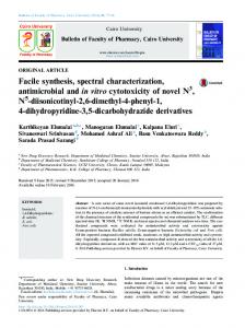
String Motion Regimes There are two main types of interaction between string and bow: sticking and slipping and its distribution in time will define the regime of motion of the string. Under Helmholtz motion regime, the time-keeping of the transitions between the two phases is determined by the traveling corner (see Figure 2.3a): • Stick: The bow is pressed against the string and pulled across it. Due to the friction of the rosin with the string, it sticks with the bow. The bow carries the string (they move with the same velocity), until the tension of the string is bigger than the friction. • Slip: The friction breaks, letting the string slip under the bow. When the string is close to the position of equilibrium, it sticks again to the bow. Depending on the actions of the performer, the temporal succession and duration of these interactions will vary and we can obtain several different regimes of motion. In ?, ? established a diagram (Figure 2.4) identifying the main regimes of motion. Among them, there is the Helmholtz motion regime, which is the most accepted model for bowed strings. It is a periodic motion where the bow slips and sticks repeatedly. This is the regime of interest in our synthesis model. Out of this region, the sound produced is not considered musically acceptable in a traditional performance. Schelleng’s diagram (Figure 2.4) shows how the Helmholtz motion can be maintained in function of the bow-bridge distance and bow force on the string, for a constant velocity. In addition to Helmholtz regime, other regions are specified, namely “raucous” and “higher modes”. Extensions of the diagram have been reported in ? where extra regimes are identified. In ? some corrections are introduced. In the process of playing a note, until the stable Helmholtz motion is reached, there is a region called pre-Helmholtz transient. Studies and simulations about the obtention

14

CHAPTER 2. LITERATURE REVIEW sticking corner

bridge

string nut

time

bridge

nut

bridge

nut

bridge

beginning of slipping

nut

t stick t slip

string displacement (under the bow)

vel. stick

vel. slip

(b) String and velocity displacement under the bow (bow is at a distance from the bridge of around 1/10 the string length). Velocity at stick phase has the same velocity of the bow and at slip phases increases.

nut

bridge

bridge

string velocity (under the bow) beginning of sticking

nut

(a) Traveling corner and stick-slip phases

Figure 2.3: String movement in Helmholtz motion.

Max

imum

bow

force

RAUCOUS

1

Brilliant Mi

Sul ponticello

1

nim

um

bow

NORMAL for

ce

Sul tasto

1

HIGHER MODES

Figure 2.4: Schelleng’s Diagram. Log-log plot, x axis is bow relative position and y-axis is bow force.

and duration of the transient have been reported by ?, ?, and ?. These transients appear during note attacks and intra-note transitions and are very important for the perception of violin sounds.

String Displacement, Velocity and Force on the Bridge In a simplified violin model, the force exerted by the strings on the bridge can be considered proportional to the sound that arrives to our ears. This force depends on the tension under which the string is kept and the angle at which the string is deflected. This angle (see Figure 2.5) is proportional to the displacement of the string (?).

2.2. VIOLIN ACOUSTICS

15

Figure 2.5: Relationship between string displacement and the amplitude of various modes of the string. From ?.

String Velocity in Time and Frequency Be β the bow-bridge distance relative to the length of the string, T0 the period of the signal, and f0 = 1/T0 . For ideal Helmholtz motion, the shape of the string velocity is a pulse train, where the pulse width is β ∗ T0 . The spectral envelope of such a signal has a shape of an absolute sinc function with nodes at n ∗ fβ0 . In Figure 2.6 we can see a square pulse and its spectrum, and the relationship among their parameters. 30

1 βT0

10

0.5 0

AβT0

20 dB

amplitude

2 A 1.5

2 fβ0 3 fβ0

1 fβ0

T0 0

50 100 time [secs]

150

0 0

5

10 15 frequency [kHz]

20

Figure 2.6: Ideal string velocity shape in time (square pulse of amplitude A and duration βT0 ) and frequency (asinc function with nodes at n fβ0 and first node amplitude AβT0 ).

Bowed string timbre Violin timbre is a multi-dimensional attribute (??) mainly determined by the frequency content of the string vibration, but also by its time history (??). Previous studies attempted to describe different violin spectra with a reduced set of descriptors (???), which allow a perceptual characterization of the timbre. However, but they are not enough to design generative models as the one proposed here (see Chapter4).

2.2.3

Radiator: Violin Body

Understanding the properties of the violin body is of great interest as it determines the sound quality of the instrument. It is usually modeled as a linear filter (???) by measuring its response to a known excitation. Depending on the type and location of both, excitation and response, different analysis can be carried out. While some studies are

16

CHAPTER 2. LITERATURE REVIEW

focused on the mechanical vibration response (???), others aim attention at the acoustic radiation (??????). In some cases, only one single response is obtained as representative of the properties of the violin body (e.g. admittance measurement, ?). However, as the body is rather a complex structure than a single vibrating element, various responses are usually measured at different points. Modal analysis techniques, for instance, measure the vibration at a grid of reading points located on the violin plates (??) and radiation patterns are obtained by recording sound pressure at different angles of the violin (????). Radiation can be measured either in the near-field (?) to study the coupling of body motion to sound energy, or in the far-field (???) to analyze the distribution of sound energy around the violin. The algorithms for computing the filter transfer function between excitation and response are typically based on signal decovolution (??). As we can realize there exist many ways to obtain violin body responses. The different approaches basically depend on the purpose of research like understanding of specific physical phenomena (?????), perceptual studies (???), progresses in violin making ? or violin sound synthesis (????). The latter commonly uses the violin body’s response as a linear filter (??) to equalize a source signal (e.g. bowed string vibration) with the main objective to evaluate specific acoustical or perceptual violin properties but not to produce realistic violin sounds. Therefore there is a need for new techniques that fill this gap. Excitation Methods The excitation signal can be impulsive (simulating a Delta) or last for some time. In any case, it must contain enough energy at all frequencies of interest to get a complete response. Hitting the violin bridge with a force hammer (?) is the most widely used impulsive excitation method. Usually the hammer is in a pendulum (?) so that reproducibility is excellent because it hits always with the same force, position and direction. The point of excitation is often at the top of one side of the bridge following the main direction of the bridge movement. Cook et al. (?) hit the violin at each of the four string-bridge notches in order to obtain a different transfer function for each string. This is also done by suddenly pulling a very thin copper wire, breaking it, which excites the string with a short impulse (?). Non-impulsive excitations are usually better against noise and measurement errors. Typical excitation signals are sinus sweep or MLS that can be applied by means of a shaker or as in the ’indirect’ method with a loudspeaker (??). ? has exhaustively described this indirect method in 1980. The shaker has to be in contact with the violin adding an extra mass which greatly influences the response. ? measure excitation with an under-saddle guitar pickup and the excitation consists of normal playing samples. Other possible methods are by finger tapping as traditionally used by violin makers, or by bowing that is the normal way to excite a violin when performing. Measuring the Response The response can either be in form of mechanical vibration or sound pressure (acoustic response). Mechanical vibration can be measured at the same point as the excitation 4 or at a different place. The most usual way is to excite the bridge at one side and measure the velocity or acceleration at the other side with an optical laser (?), with an 4 Versatile Instrument Analysis System. http://www.bias.at/

2.2. VIOLIN ACOUSTICS

17

accelerometer (?), or even with a magnet inside of a coil (?). The clear advantage of using a laser is that no extra mass is added to the bridge. Acoustic response is measured with a microphone, ideally in an anechoic chamber so that no effect of room reverberation is included. One problem that comes up when measuring the acoustic response is that usually the excitation itself produces mechanical sound (e.g. hitting the bridge). For synthesis purposes, the acoustic response is definitely more adequate as high values of surface mobility may not produce high-energy output, but rather energy sinks. Furthermore, sound radiation may have contributions from the air cavity through the f-holes, not measured by plate vibration analysis (?). However in ?, admittance measures are used for synthesis to carry out perceptual studies. In some cases one single response is measured as representative of the whole body (?). However, as the body is rather a complex structure than a single vibrating element, various responses are usually measured at different points. Modal shapes of violin plates have been studied in ???. Modern interferometry systems 5 are able to measure vibration at multiple points simultaneously and sound radiation patterns are obtained by measuring sound radiation at different angles around the violin (??????). Representation of the Body. Several possibilities are used to parameterize the model of the body: • Sampled impulse response of the body or frequency response: Recordings of the body after being excited by an impulse, that is, the impulse response of the body or its Fourier transform. This is the approach that we will use. • Linear time-invariant Filter Approximation: Several techniques are known that approximate the impulse response of a resonant body with a filter (?). • Modal analysis/synthesis is basically a collection of parallel high-resonance bandpass filters, excited by an input impulse. Each filter has three parameters: frequency, resonance (decay time), and output level. It is especially good for simulating struck sounds, like rods, bars, and plates, and objects with low number of modes. As the violin has a very high number of modes (especially in the high frequencies), this method could allow to approximate the low frequency modes in the violin. Violin Body Resonances The response of the violin is characterized by its resonances or modes, and can be visualized as peaks in the magnitude spectrum. The way of identifying the modes of the violin described in ?, has become a standard in the field. They classify the modes as follows: • A modes, caused by the motion of enclosed air. When the body is vibrating, the volume of the body is changing and air is pressed out and sucked into. The A0 resonance corresponds to the resonant frequency of the whole volume resonator. • B modes, are motion modes of the back plate. 5 Like the interferometry laser laboratory at IWK (Institut für Wiener Klangstil) http://iwk.mdw.ac.at/

18

CHAPTER 2. LITERATURE REVIEW • T or P modes, are due to motion primarily of the top plate. • C modes, refer to bending and flexing modes of the “corpus” or body. • N mode, is the resonance of the neck. • BH is the so called bridge-hill and represents the resonances of the bridge, which overlap and form the shape of a smoothed hill (not a peak) between 2 and 3kHz.

The main violin resonances are represented in Figure 2.7. The air resonance (A0), around 270Hz, T1 between 400 and 500 Hz, C3 between 500 and 600 Hz and BH (Bridge hill) between 2 and 3kHz. Violin Bridge admittance 30

energy[dB]

20

Mode T1 (~460Hz)

Mode C3 (~530Hz)

Bridge Hill (~2−3kHz)

Mode C4 (~800Hz)

10 0 −10 Mode A0 (~275Hz) −20

500

1000

1500 freq[Hz]

2000

2500

3000

Figure 2.7: Bridge admittance curve to show the main violin resonances. There are different nomenclatures for the modes. We use here one of the most typical. Mode A0 (air cavity resonance) is not very prominent in the admittance curve but is perceptually relevant. The Bridge Hill is an area between 2-3 kHz with a high density of modes from the bridge.

Acoustic Radiation Acoustic radiation from violins has been extensively studied by ? and ?. Sound is radiated from the violin in all directions. Radiation is a very complex phenomenon that depends on the properties of the source producing the sound, in particular on its size and frequency. The relation size/frequency determines largely the properties of the radiation. For a diameter (meters) of the sound source smaller than 100(Hz × m)/ f requency(Hz) (DG measure, as defined in ?), the sound is radiated with equal strength in all directions, and for a longer diameter the radiation becomes more directed and complex. This can be easily seen in the spectra of sounds recorded at different directions and positions. At low frequencies little sound is projected and at higher frequencies most of the sound is radiated. Sound radiation in a plane around the player is represented in Figure 2.8 taken from ?. Studies can be categorized in two groups: near-field techniques which analyze the relation between body motion and sound radiation, and far-field techniques which measure the overall radiation independently of which modes are being excited. Most of the reported studies concentrate on the frequency response. ? loudness curves and long-term-average

2.2. VIOLIN ACOUSTICS

200-500 Hz

1000-1250 Hz

19

550-700 Hz

1500 Hz

800 Hz

2000-5000 Hz

Figure 2.8: Main radiation directions for the violin, after Meyer. Taken from ?.

spectra (??) provide pressure magnitude as a function of frequency. Other studies concentrate on the full-field acoustic intensity (magnitude and direction) usually based on the NAH technique (near-field acoustical holography) (?). In general the analyzed data is available for a limited range of low frequencies and we need the response over the full range of frequencies in the order to obtain realistic sounds.

Source plus Filter Synthesis Violin sound synthesis based on a source plus filter (body impulse response) approach is often used in the field of violin acoustics, although in most of the cases the final objective is not to produce high quality sounds. This is the case of many perceptual studies which are focused on the analysis of certain sound properties. ? report a perceptual analysis about directivity of violin timbre and ? realize psychoacoustic experiments with virtual violins. ? investigate modifications of the resonances of violin body modes. Other works report violin body models which are evaluated by filtering some source signal. For instance, ? applies filter design techniques to model violin body resonances that are used together with a physical model of string vibration; ? describe new techniques to model reverberant instrument body responses based on auditory models and ? make use of Waveguide Meshes to model high frequency violin body resonances. For spatial audio rendering, the wave field synthesis is the most related procedure. In ?, responses are obtained by the inverse method and a synthetic sound is reproduced with 6 digitally processed speakers (La timé). The most related approach to our research is by the described by ? who designed a method to obtain an acoustic sound from the signal of a guitar pickup.

20

CHAPTER 2. LITERATURE REVIEW

2.3

Performance Gestures

Acoustical studies of the physical controls of the violinist and their effect on the sound produced (?) show that the main control parameters of a violin are bow speed, distance between bow and bridge and bow force. Other parameters such as string being played and fingering can be extracted directly from the spectral analysis as reported in ?. Some other important parameters such as bow-hair width in contact with the string, resin or bow tilt are very difficult to measure and no reports are found.

Figure 2.9: Main violin controls. Upper Figure is taken from ?.

2.3.1

Bow Position, Velocity and Acceleration

The main methods reported in the literature to capture gestures of bowed-string instruments are the following: • With electrified strings and bow. The first attempts to measure bowing gestures are reported by Askenfelt in ? and ?, where bow position is detected by means of a thin resistance wire inserted among the bow hairs which makes contact with the electrified strings. The bow wire is divided in two parts by the string, each of those parts constituting one branch of a Wheatstone bridge. The same way, the string is divided in two parts by the wire, to constitute the other two branches of the bridge. • Based on capacitive sensing, a technique part of a broader one called electric field sensing, where oscillators driving antennas are mounted on the bridge and track

2.3. PERFORMANCE GESTURES

21

the position of the bow (???). This is a similar to the capacitance measurements used in the Theremin. • Accelerometers are used by ? to measure bow acceleration from which velocity and position can be obtained. In Figure 2.10 there is a detail of the accelerometer attached to the bow. In ? the same system is improved with the help of video cameras. • A Polhemus motion tracking system, adapted to the violin. This is our developed system that is fully described in Section3.3.1. • A Vicom multi-camera system, is adapted to acquire violin gestures by ? follows are own geometrical approach for parameter computation.

Figure 2.10: Wireless system for measuring bowing acceleration: Hyperbow from IRCAM.

Systems based on capacitive sensing seem to be more intrusive, the sound obtained
in the system developed by ?? can not be used for synthesis purposes because the wire in the bow makes contact with the string. Accelerometers seem promising but they only provide acceleration with no information about the direction. The system using the Vicon 6 cameras is more intrusive and needs a lot of post-processing, which makes it difficult to use in real time.

2.3.2

Bow Force

According to the literature, the best way to measure the pressing force that the bow produces on the string seems to be by means of strain gages. Bow force is meant to be the force exerted by the bow on the string, but due to the complexity of measuring it, alternative solutions that give an approximation to this parameter are found in the literature: • Force exerted by the violinist with the forefinger. This can be achieved by fixing a Force Sensing Resistor on the bow under the forefinger of the player. This approach is used in ? and ?. 6 VICON

systems: http://www.vicon.com/

22

CHAPTER 2. LITERATURE REVIEW • Bow-stick strain. In ? they fix two strain gauges at the middle point of the bow, in two directions, to capture downward and lateral strain of the bow stick. See Figure 2.11. • Bow-hair strain. In ?? they use a pair of strain gauges at both ends of the bow hair, and compute the bow force using a Wheatstone bridge. In a similar way to the setup described in ? and ?, we fixed the gages on a metallic surface under the hair ribbon in the frog of the bow, and connected to a Wheatstone Bridge and an amplifier.

Figure 2.11: Hyperbow from MIT (?).

2.4

Expressive Performance Models

Modeling expressive performances is an active research topic. The main computational approaches used for modeling expressive performances are summarized next:

2.4.1

Analysis by Synthesis

This approach is used by ?. They define a set of performance rules that model different expressive features like phrasing, note grouping. These rules are proposed by human experts, and are refined through process called analysis by synthesis, in which comparisons of real performances with the predicted by the set of rules are recursively made.

2.4.2

Automatic Learning Techniques

In this group we include performance models that apply techniques of Artificial Intelligence such as machine learning and data mining in order to gather performance rules. In ?, authors apply these learning techniques to articulations and dynamics in musical performances. ? has derived a number of performance principles from a large set of piano performances of Mozart sonatas. The models are typically in the form of rules that predict expressive deviations based on local score context. An advantage of this method over analysis by synthesis is that no prior hypotheses have to be specified, rather the

2.5. MACHINE LEARNING TECHNIQUES

23

hypotheses are extracted from the data. Model generation using inductive algorithms is subject to a trade-off: on the one hand predictive models can be derived to maximize predictive power. Such models provide a high predictive accuracy due to the induction of a large set of highly complex rules that are generally unintelligible. On the other hand, the induction of descriptive models involves a conservative approach to the introduction of rules, trying to keep the complexity of rules as low as possible, at the cost of reduced accuracy. ? make use of inductive machine learning to predict onsets, duration, and dynamics. This is basis for our expressivity models. Genetic algorithms are also used to model expressive time and dynamics deviations by ?. ? makes use of artificial neural networks that try to imitate the expressive style of analyzed piano performers.

2.4.3

Case Base Reasoning

This is an alternative technique to the automatic rule induction technique. Instead of generating a set of rules in an analysis phase, it uses the most similar examples (called cases) directly to process new melodic material. SaxEx (?) is a CBR system that generates expressive music performances by using previously performed melodies as examples. ? proposes a case base reasoning approach to make expressivity-aware tempo transformations of music performances. Another example of a CBR system for expressive music performance is Kagurame, proposed by ?. This system renders expressive performances of MIDI scores, given performance conditions that specify the desired characteristics of the performance.

2.4.4

Melodic Structure: Narmour Groups

In section 6.6, we present an expressivity model based on the melodic structure defined in the theory of ?, known as the Implication-Realization (I-R) model. It is based on the idea that when a listener is hearing a melody, always generates expectations on how to continue. According to Narmour, these expectations are driven by innate and acquired mental processes. Furthermore, the influence of the musical environment of the listener throughout his life also affects these expectations. Based on this idea, Narmour explains that in music made by humans there are certain rules that are often repeated. These rules are based primarily on two characteristics: 1) the principle of interval difference (PID): a small interval (five semitones or less) implies a similar one (with a margin of two semitones), and a large interval implies a smaller one, and 2) the principle of registral direction (PRD), states that small intervals imply an interval in the same registral direction. The eight main I-R patterns considered by the theory of Narmour are specified in Figure 2.12.

2.5

Machine Learning Techniques

Here is a short description of the main machine learning algorithms used in this dissertation 7 . A brief description is included here as an introduction and reference for the 7 Machine

Learning frameworks used in this work:

Weka: http://www.cs.waikato.ac.nz/ml/weka/

24

Violin

  

CHAPTER 2. LITERATURE REVIEW

  P

   D

   ID

   I

P

  VP





 



R

  I

R







VR

(a) Main Narmour Groups

Structure P D ID IP VP R IR VR

Interval sizes SS 00 S S (eq) SS SL LS LS LL

Same direction? yes yes no no yes no yes no

PID satisfied? yes yes yes yes no yes yes no

PRD satisfied? yes yes no no yes yes no yes

(b) Narmour structures description

Figure 2.12: Basic Narmour I-R structures. In the second column, ‘S’ denotes small, ‘L’ large, and ‘0’ a prime interval.

following chapters. Artificial Neural Networks. An Artificial Neural Network (ANN) is a non-linear statistical data modeling tool that is inspired by the way biological nervous systems, such as the brain, process information. They can be used to model complex relationships between inputs and outputs or to find patterns in data. They are composed of a group of interconnected processing elements (neurons) working in unison to solve specific problems. They are configured through a learning process in which synaptic connections that exist between the neurons are adjusted based on external or internal information that flows through the network. Neural networks have been widely used for prediction or forecasting in various fields. An excellent introduction to the field of neural networks is found in ? and a more detailed survey of basic neural network architectures and learning rules in ?. Most of the figures representing Neural Networks are taken from the MATLAB documentation or based on its particular representation. The simplest processing element called neuron is represented in Figure 2.13a. The neuron has a single input p a connection with an associated weight w and a transfer function f. The input is transmitted through the single connection that multiplies its strength by its corresponding weight w. The weighted input wp is the argument of the transfer function f, which produces the output a. A more general case is depicted in Figure 2.13b with a vector of inputs and an extra internal connection called bias. The output of the neuron is f (∑ wp + b). Many transfer functions f are possible. The most typical ones are the step, linear and log-sigmoid. LibSVM: http://www.csie.ntu.edu.tw/~cjlin/libsvm/ Neuralnet MATLAB toolbox: http://www.mathworks.es/products/neuralnet/

2.5. MACHINE LEARNING TECHNIQUES

25

(a) Simplest neuron. It has a single input p a connec- (b) General neuron scheme with a vector of intion with an associated weight w and a transfer puts p = {p1 , p2 , ..., pR }, their corresponding function f. weights W = {w1 , w2 , ..., wR } and a bias b.

Figure 2.13: Single neuron. Many transfer functions f are possible. The most typical ones are the step, linear and log-sigmoid. The value of the output a is indicated. Figures are from MATLAB documentation.

Neurons are connected forming a network. The architecture of the network can have any shape but the most usual configurations are feed-forward networks where all connections go forward and there are no loops. These configurations are typically structured in neuron layers as shown in Figure 2.14a. A simplified representation of the same network appears in Figure 2.14b. Another typical simplified representation is as circles as used in the following chapters. Networks are trained with examples of real data and weights of the neurons are adapted to minimize the error at the output. The most typical training algorithm is backpropagation. Feed-forward networks are considered to be static because the output is calculated directly from the input through feed-forward connections. Another type of networks is dynamic networks, which is largely used to model dynamic systems. These networks contain feedback elements or delays. The output depends not only on the current input to the network, but also on the current or previous inputs, outputs, or states of the network. The networks used in this research are Focused Time-Delay Networks which are feed-forward networks with tapped-delays in the input, so that they depend on previous inputs; Nonlinear Autoregressive Network with Exogenous Inputs (NARX) (see Figure 2.15), which also has a tapped delay at the inputs and outputs have feedback connections to the input layer. Support Vector Machines (SVM). It is a useful technique for data classification, although it can be used for regression as well. Here training vectors are mapped into a higher dimensional space (even infinite) by a kernel function. Then a SVM finds a linear hyperplane or a set of hyperplanes that separate the different classes of the training data in the higher dimensional space. Intuitively, a good separation is achieved by the hyperplane that has the largest distance to the nearest training data points of any class (so-called functional margin), since in general the larger the margin the lower the generalization error of the classifier. The advantage of this technique is that the cost function for building

26

CHAPTER 2. LITERATURE REVIEW

(a) Detailed scheme showing all the connections.

(b) Simplified representation as matrices.

Figure 2.14: Two representations of the same Feed Forward Network with three layers l = 1, 2, 3. Each layer has a number of neurons Sl = 3. The network has an input vector p with R elements that are connected to each input-layer’s neuron with the corresponding input-weights matrix IW of size S1 xR. The output of each layer is a vector al of size the number of neurons in the layer Sl . Layer connections weights LW are matrices defined similar to the input-weights IW. Figures are from MATLAB documentation.

the model does not care about training points that lie beyond the functional margin, so the cost is independent of the size of the training data. There are four basic Kernel functions: linear, polynomial, radial basis function and sigmoid. An overview of the basic ideas underlying Support Vector Machines for regression can be found in ?. Inductive Logic Programming (ILP). It is a subfield of machine learning which uses logic programming as a uniform representation for examples, background knowledge and hypotheses. Given an encoding of the known background knowledge and a set of examples

2.5. MACHINE LEARNING TECHNIQUES

27

Figure 2.15: NARX recurrent network architecture. It has a recurrent connection which feeds the output back to the input. Additionally, it has a tapped delay line (TDL) to make n previous input vectors available as input. Figure is from MATLAB documentation.

represented as a logical database of facts, an ILP system will derive a hypothesized logic program which entails all the positive and none of the negative examples. This technique has the advantage over the last methods that it develops prediction predicates (hypothesis) that are human readable, which can be very informative to better understand the modeled system. A description of ILP techniques and its applications is ?. Gaussian Mixture Models. Gaussian Mixture Models (GMM) are non-supervised statistical models widely used for clustering and density estimation, but also for regression as is our case. They consist of a mixture of normal (Gaussian) distributions each one with a mean and a covariance matrix (one variance for each of the space dimensions). The mixture distribution parameters are optimized to obtain the maximum likelihood by means of the iterative algorithm Expectation-maximization. It is an iterative algorithm with two steps: an expectation step and a maximization. E-M algorithm stops when it converges (likelihood increment during an iteration is lower than a threshold). More details about GMM are found in ?.

CHAPTER

Techniques for Measuring Violin Performances This chapter describes the techniques developed for measuring synchronized audio and gestures during real violin performances. A set of musical scores is designed with the aim of covering the most common violin playing contexts. All the scores are performed and recorded with the measuring system in order to build a database of audio and performance actions used for analysis (Chapter 4) as well as for synthesis (Chapter 6). The sensing system is fully described in previous publications (???). The work described in this chapter was done in collaboration with Merlijn Blaauw, who implemented the algorithms and developed the software for capturing, visualizing and synchronizing all data and Enric Guaus, responsible for the force measurements with the gages. The conception of the bowing motion capture system was done together with Esteban Maestre and Jordi Bonada.

3.1

Recordings Setup

During the recordings, audio synchronized with motion data is captured and stored in a performance database which is used for both analysis (to build the models) and synthesis. The general procedure is schematized in Figure 3.1. As described in the following sections, data is captured with different sensors (in red): Two motion sensors that track bow and violin motion, a strain gage that measures bow pressing force and a bridge pickup to measure bridge vibration. Synchronization of different types of data is done via a VST-plugging used in the recording software (Cubase/Nuendo 1 ), which sends a clock signal to the different devices. The plugging visualizes a 3D representation of the position of the violin and bow in real time, as well as some performer actions curves which are useful to follow the performance and detect possible errors during the calibration or the recordings. In Figure 3.2a there is a picture of a typical recording session. Additionally, one microphone is used during the recordings as a reference and two video cameras that provide extra visual information that may be useful in the future. 1 http:\www.nuendo.com

3

30

CHAPTER 3. MEASURING VIOLIN PERFORMANCES

visualization

VST plugging

Polhemus system clock

Arduino

Violin motion Bow motion Hair ribbon strain

Audio (pickup) Synchronized data

Figure 3.1: Recording setup scheme. VST plugging synchronizes all data streams (audio from the pickup, motion from the Polhemus and strain from the gages) and stores them.

3.2

Score Design

Scores are designed to cover the most common violin playing contexts (traditionally speaking) while having a relatively small database. At the same time, scores have to be musically meaningful and if possible familiar to the player. In Figure 3.3, the bigger circle represents all the sounds which can be produced with the violin. The smaller one represents the playable region of interest, which in our case are traditional performances. Small trajectories inside this region represent the recorded samples. Any trajectory can be slightly modified by applying different sound transformations, without loose of sound quality, so that each trajectory covers a small region of the playable space. The objective of score designing is therefore, to find a small set of trajectories that maximize the coverage of the region of interest. Samples consist of whole musical phrases taken from violin repertoire instead of isolated notes based on the idea of performance sampling (?). Score generation is done in two recursive steps: 1) small music motifs or source snippets are selected from violin repertoire by an expert. They cover the main features in violin playing technique (i.e bow strokes, bowing patterns, dynamic changes, string changes, etc.) and manual selection guarantees that selected motifs are playable and musically interesting. 2) an algorithm automatically populates the playable space by transforming the manually selected motifs into similar ones with different dynamics, note durations, strings, fingering positions and pitches, while keeping the playability of the new excerpts. The general scheme is depicted in Figure 3.4. Snippet selection and coverage computation is done separately for short (or fast) notes (eighth notes and shorter ones and long (or slow) notes (fourth, half and whole), because they are used in very different contexts. Snippets are played without vibrato (it will be synthesized), avoiding accents and dynamic changes which will be modeled as patterns.

3.2. SCORE DESIGN

31

(a) Recording session.

(b) Plugging screenshot in Nuendo. Real time 3D representation of violin and bow position and visualization of several bowing parameter contours.

Figure 3.2: Photograph during a recording session and 3D violin model visualizing the movements of the performer.

3.2.1

Coverage

In order to simplify the algorithm, coverage is restricted to groups of two notes and the following features: Note Transition Features Transition features are mainly determined by the bow stroke (or articulation). The most common bow strokes in violin repertoire are specified in Table 3.1.

32

CHAPTER 3. MEASURING VIOLIN PERFORMANCES Region covered by the trajectory by applying sound transformations A possible sounds produced by the instrument B musically relevant sounds produced by the instrument

recorded audio samples Figure 3.3: Playable space representation.

From all bow strokes, we focus on the most common ones: legato, detaché, staccato and saltato. The others can be considered variations of these basic ones. For example, portato is a legato with accents and spiccato a shorter saltato with a more crispy sound. The core of the database corpus is composed of legato and detaché notes where transitions play a very important role. Notes played with other articulations (staccato and saltato) are considered isolated notes without transitions. The main note-to-note transition features identified are: • Articulation: The possible two note combinations with detaché and legato are: – detaché → detaché, two consecutive detaché notes. – detaché → legatob , first note is detaché and second note is the beginning of a legato. – legatoe → detaché. First note is the end of a legato and second note is played detaché. – legato → legato – legatoe → legatob – silence → note (phrase start) – note → silence (phrase ending) • String change: Changing the played string between two notes makes them sound different than when played in the same string. Only changes to adjacent strings are considered. • First note finger position: All starting positions at each string must be present in the database. The grid size is a semitone. • Note interval: Together with the ending string determines the second note finger position. For each starting position all ending positions have to be evenly sampled (until one octave for the same string). Large intervals require hand position change which often result in small audible glissandi.

3.2. SCORE DESIGN

33

Classical score collection

transpose •String position •Finger position

… … … Expanded snippets: all possible transpositions of the motifs.

Motifs or source snippets

Find optimal combination

Coverage statistics

Recording script

Figure 3.4: Overview of the recording script generation process. Notice how the third source snippet and four of its transpositions form the first generated phrase.

Intra-Note Features These features are not included in the coverage algorithm, but are still covered in other ways. • Note accents: Can have different intensity (hard, soft), duration (long, short) and position inside the note (beginning, middle, end). Different attacks are recorded and considered as templates that can be applied to any note as a sound transformation. • Note duration or tempo. We classify groups of notes as fast or slow and coverage is computed separately. We assume that intermediate durations can be obtained

34

CHAPTER 3. MEASURING VIOLIN PERFORMANCES Bow Stroke

Description

Legato

Smoothly connected notes, in the same bow.

Portato

Short series of gently pulsed legato notes.

Detaché

Each note in a separate stroke, with constant speed and smooth attack

Staccato

Shortened detaché with initial accent, the bow remaining on the string. Often used with slurs, as a series of short stopped notes played in the same bow.

Martelé

Almost a percussive attack followed by quick release. The notes are separated, and bow remains on the string.

Spiccato

Off-the-string, bouncing bow stroke, producing a crisp sound.

Staccato Volante

Bouncing bow stroke, short notes, usually during up-bows.

Staccatissimo

As staccato but with shorter notes.

Table 3.1: Most common violin bow strokes.

with time stretching transformations. A third class of note duration is very long notes, considered a special case with specific scores dedicated. • Note dynamics. To cover dynamics, generated scores are played in three dynamics: piano, mezzoforte and forte. Intra-note crescendo and decrescendo are recorded as templates, not considered for the coverage.

3.2.2

Manual Snippet Selection

In this step, small fragments of musical scores (source snippets) are selected. The final scores are a combination of source snippets and transpositions of them, so it is a crucial step in order to ensure that the generated scores be musically meaningful and that they contain the most common playing contexts. The main sources for the selection are classical violin repertoire, and the compilation of the most important bowing patterns in ?. Selection is carried out separately for long and short notes. Special care is given to string and position changes, trying to cover most combinations. As coverage computation

3.2. SCORE DESIGN

35

considers only groups of two notes, this step is responsible for including relevant gestures involving several notes, which is specially important for the case of short notes, where common bowing patterns comprise several ones. Each note in the source snippets is annotated with the string to be played on. Fingering, that is, which finger is used to play each note, is not relevant and can be freely chosen by the performer. Given the string and pitch of a note, the corresponding finger position (on the string) is obtained. It is measured in semitones, being semitone zero the open string. As special cases, scales and arpeggios are also added to the source snippets for short notes: • Three-octave scales and arpeggios. Fast fragments similar to scales or arpeggios are extensively used in violin repertoire. Diatonic and chromatic scales are recorded for combinations of detaché and legato. • One-octave scales in the same string. These scales contain several hand position changes in the same string. There are versions for detaché and legato.

3.2.3

Automatic Snippet Generation

Snippet Transposition The extension of a snippet is given by its lowest and highest string and its minimum and maximum finger position. Source snippets can be transposed into similar ones by shifting them to different strings or finger positions, but always keeping relative fingering and string changes. This way a source snippet can cover several pitches and strings while keeping its playability. Snippet extension determines its possible transpositions. (i.e a snippet using G-string in any of its notes, can’t be shifted to a lower string). Transpositions are also restricted by physio-mechanical constraints of the instrument (for instance, certain pitches can’t be played on certain strings) and finger position changes are limited by playability and readability of the resulting scores: the exact number of semitones of the transposition depends on the number of sharps and flats they produce (less is better), so if a transposition has many a close transposition with less accidentals is used. Transposing motifs so that a fingered note becomes an open string note and vice-versa is not allowed as it effectively changes fingering of the motif. Source snippets and all their possible transformations form together the expanded snippets. We count with sound transformations, which allow one pitch to also cover pitches nearby (currently 3 semitones up and down) so a certain snippet covers a small region around itself. Optimal Snippet Set From all the expanded motifs, the optimal set (recording script) is obtained by computing the coverage of each of the expanded snippets and their playing time and selecting the optimal one. This is repeated iteratively until the maximum playing time is reached or when there are no more remaining extended motifs. Internally the system computes the coverage using a kind of multi-dimensional histogram. The application can visualize this histogram which is useful for finding out what kind of motifs are missing. Open string coverage is calculated separately. In Figure 3.5 we show a fragment of such a coverage histogram. In the left part of the table, note duration and type of articulation is indicated, as well as string and finger position (semitones) of the first note. At the right, all possible

36

CHAPTER 3. MEASURING VIOLIN PERFORMANCES

combinations for the second note (string and finger position) appear. The four main divisions indicate second-note-string. Each division has 25 sub-columns corresponding to finger positions (2 octaves). Each position is filled with a textual character indicating the degree of coverage: • A point ’.’ indicates a gap in the generated optimal set. • A lower-case ’o’, indicates that a snippet in the optimal set covers that position through sound transformations (i.e pitch shift or time stretch). • An upper-case ’O’, indicates that at least one snippet is covering that position. • A blank space indicates that the position is impossible or not considered. For instance, in Figure 3.5, the first note is played on the first string. As only changes to adjacent strings are considered, divisions for the 3rd and 4th string are blank. Finger position is limited to two octaves for the first string and to one octave for the rest. The algorithm outputs the optimal motifs, and a score of gaps (note transitions not covered in the generated scores). Gaps are used to manually make new snippets and together with the source snippets, are recursively given to the algorithm that will produce a new score with larger coverage, and new gaps that may still be missing. The resulting recording script is sorted in such a way that is easy to play for the violinist. For instance, the transpositions of all the motifs always happen in the same order. All transpositions of one snippet are combined in the same phrase, which is recorded in one take. One of the requisites is to generate a score of no more than 45 minutes, so there is a tradeoff between score length and coverage. Coverage was around 70% for short notes and 60% for long notes.

3.2.4

Special Scores

Certain types of musical contexts were not covered by the above automatic score generation method and did not require such a systematic approach. Normally these scores contain either isolated notes which have no note-to-note transition or certain types of expressive feature that are used as a template. These scores were created by hand: Very long notes. Covering most of the pitches in each string (each third approximately). There are also crescendos and decrescendos used as templates. Vibrato templates. We are not interested in pitch but in pitch modulation. We consider long and short notes, different dynamics and moods. Isolated notes. Staccato, saltato and spiccato notes are considered to be isolated without transitions between notes. Only a 3-octave scale at different dynamics is needed. Harmonics and pizzicato. They are treated the same way as isolated notes, but they are handled differently during the synthesis because they have a long queue: They do not have duration, and there is no time stretch. Ornaments. Trills, tremolo, mordents, turns and glissandi. They are considered as templates.

3.3. PERFORMER ACTIONS

37

Notes duration Transition type (articulation) Note1 (string and finger position)

Note2 ( all string and finger position combinations )

E-String (1st)

A-String (2nd)

D-String (3rd)

slow; det-det; (str = 1, semitone = 0) slow; det-det; (str = 1, semitone = 1) slow; det-det; (str = 1, semitone = 2) slow; det-det; (str = 1, semitone = 3) slow; det-det; (str = 1, semitone = 4) slow; det-det; (str = 1, semitone = 5) slow; det-det; (str = 1, semitone = 6) slow; det-det; (str = 1, semitone = 7) slow; det-det; (str = 1, semitone = 8) slow; det-det; (str = 1, semitone = 9) slow; det-det; (str = 1, semitone = 10) slow; det-det; (str = 1, semitone = 11) slow; det-det; (str = 1, semitone = 12) slow; det-det; (str = 1, semitone = 13) slow; det-det; (str = 1, semitone = 14) slow; det-det; (str = 1, semitone = 15) slow; det-det; (str = 1, semitone = 16) slow; det-det; (str = 1, semitone = 17) slow; det-det; (str = 1, semitone = 18) slow; det-det; (str = 1, semitone = 19) slow; det-det; (str = 1, semitone = 20) slow; det-det; (str = 1, semitone = 21) slow; det-det; (str = 1, semitone = 22) slow; det-det; (str = 1, semitone = 23) slow; det-det; (str = 1, semitone = 24) 0 1 2 3 4 5 6 7 8 9 10 11 12 13 14 15 16 17 18 19 20 21 22 23 24

0 1 2 3 4 5 6 7 8 9 10 11 12 13 14 15 16 17 18 19 20 21 22 23 24

Finger position in string (semitones)

Figure 3.5: Fragment of a score coverage histogram corresponding to detaché transitions of slow notes. Table shows all possible string and finger-position combinations when the first note is played on the E-string. 0 1 2 3 4 5 6 7 8 9 10 11 12 13 14 15 16 17 18 19 20 21 22 23 24

Accent templates. Notes with accent at the beginning (maretelé, sforzando), at the middle (tenuto) and at the end.

3.3

Performer Actions

We understand by performer actions, the musically producing gestures that the violinist executes during a performance, such as bow velocity, bow pressure or finger position. This section is dedicated to the developed measuring system for performance actions acquisition. Actions are measured with two types of sensors: a commercial 3D motion tracking system (Polhemus Liberty System 2 ) to measure bow motion and an own-built device based on strain gages to measure bow force. A preliminary sensing system presented in ?, is described in Appendix B. 2 Polhemus

Liberty System http://www.polhemus.com

01234

38

CHAPTER 3. MEASURING VIOLIN PERFORMANCES

3.3.1

Bow Motion

Bow motion is obtained with a commercial 3D tracking system (Polhemus Liberty system). The system consists of a source, an approximately 10x10x10 cm cube which generates an electro-magnetic field (EMF), a set of small sensors or trackers and a signal processing box to which source and sensors are wire-connected. More details can be found in ?. When the source is emitting the EMF, the system can determine position and orientation of each sensor inside the magnetic field. The signal processing box can perform tasks like noise reduction and various coordinate system conversion tasks. It is connected to the host PC using USB (or serial communication port) and can be programmed through a supplied SDK. The most important specifications of the system are as follows: • A sample rate of 240 Hz. • Static position accuracy 0.71 mm (RMS). • Static orientation accuracy of 0.15 degrees (RMS). • Static position resolution of 0.038 mm with source-sensor distance of 91 cm. • Static orientation resolution of 0.0048 degrees with source-sensor distance of 91 cm. • Workable-range around 1.5 meters. The resolution of the system is dependent on distance between source and sensors (noise and resolution grain increase nearly exponentially with distance), so we try not to exceed a range of around 1.5 meters. Dynamic accuracy (sensors are not static but moving) deteriorate as well. Nevertheless the system provides a really good accuracy and resolution for our application. We use three different kinds of sensors: 1. A sensor (S1) with box-shaped plastic enclosure. The enclosure makes it easy to attach to other objects and protects the sensor of possible mishaps. It is attached to the back of the violin body, see Figure 3.6. 2. A second sensor (S2) with a tear-drop shape. This sensor is smaller and thinner and is attached to the bow stick, see Figure 3.6. 3. A stylus sensor (Figure 3.7). This sensor has a pen shape with a factory calibrated needle metal tip. It also features a button which can be used to trigger taking single points. Sensor placement on the instrument has been chosen to minimize intrusivity when performing.

3.3. PERFORMER ACTIONS

39

Figure 3.6: Detail of Polhemus sensors placement on violin body (top) and bow (bottom).

Calibration At each instant the system is providing the position and orientation (Euler angles) of the sensors with respect to the source. Any point in the space can be expressed as source coordinates or relative to any of the sensors. System coordinates of a sensor (Si ) (which change at each instant) are defined by the tuple position (Psi ) and rotation matrix (Rsi ). Position(Psi ) is obtained directly and rotation matrix(Rsi ) is computed from the Euler angles (azimuth (az), elevation (el) and inclination (inc)): Rsi = rotz ∗ roty ∗ rotx, where rotz, roty and rotx are the Euler rotation matrices 3 specified in eqs. 3.1, 3.2 and 3.3. cos(az) − sin(az) 0 rotz = sin(az) cos(az) 0 (3.1) 0 0 1 cos(el) 0 sin(el) 0 1 0 roty = (3.2) − sin(el) 0 cos(el) 1 0 0 rotx = 0 cos(inc) − sin(inc) (3.3) 0 sin(inc) cos(inc) Any point in sensor coordinates psi is expressed in source coordinates as p = psi ∗ Rsi + Psi

(3.4)

psi = (p − Psi ) ∗ R−1 si

(3.5)

or equivalently:

We fix the violin sensor (s1) to the back plate of the violin at the button of the neck (Figure 3.6). In this position it is not intrusive and it does not affect the sound. Bow 3 http://mathworld.wolfram.com/EulerAngles.html

40

CHAPTER 3. MEASURING VIOLIN PERFORMANCES

sensor (s2) is attached to the top of the bow stick (Figure 3.6), near the center of gravity to keep the balance of the bow. A calibration is needed to know the position of the strings with respect to the violin sensor (S1) and the position of the hair ribbons with respect to the bow sensor (S2). The process consists of ‘sampling’ the string ends and hair ribbon ends with the stylus sensor. Relative coordinates of these points are constant during the whole performance as violin and bow are (almost) rigid objects. For any position and rotation of the sensors at any time of the performance, we can obtain the coordinates of the calibrated points with respect to the source coordinate system, by applying eq. 3.4. This way we know the position of the strings and bow hair ribbon with respect to the same coordinate system.

Figure 3.7: Polhemus Liberty system stylus sensor and close up of the sensor’s tip used during the calibration.

The calibration points are specified with circles in Figure 3.8: • String ends: from the string anchorage on the bridge to the top nut notch. • String projection on the beginning of the fingerboard. These can be used to identify the beginning of the fingerboard as well as the point of maximum string inflexion caused by the pressing finger or the bow. As we do not consider string or bow hairs deformation yet, these points are not used. • Hair ribbon ends: At the tip and frog on the right and left sides. Only the left hair ribbon side is used at the moment to compute bowing descriptors. Below, when referring to hair ribbon line we mean the hair ribbon’s left side. Playing String Detection Once the strings and hair ribbon are calibrated, we proceed to obtain the performer actions. The first step is to detect which string is being played. We have devised a method based on measuring the angle of the left hair ribbon line, and the violin plane: first, we obtain the plane of the violin from the ends of the outer strings. Then, we compute the angle

3.3. PERFORMER ACTIONS

41

Figure 3.8: Points marked during the calibration process: String ends, bow hair ribbon ends and fingerboard end.

between the hair ribbon line and this plane (see Figure 3.9). From the computed angle, we are able to obtain a good estimation of the string being played.

Figure 3.9: Motion descriptors: Bow inclination, angle between violin horizontal plane and hair ribbon. Used for automatic detection of the string being played.

For the detection of the angle limits we carry out a short recording while computing bow inclination. The recording consists of playing the score in Figure 3.10), which contains 7 different angle-segments: one for each string (G,D,A,E) and one for the three possible combination of double strings (G+D, D+A, A+E) played changing the angle gradually: G-GD-D-DA-A-AE-E. All segments are played at different dynamics and durations and the whole bow length is used. After a manual segmentation of the 7 segments we obtain typical values for inter-string angle limits: αEA = 15◦ , αAD = −2◦ , and αEG = −19◦ . Figure 3.11 shows an example of single and double string detection for a recorded fragment containing all the 7 segments consecutively. From top to bottom: recorded audio coming from the pickup, inclination angle, and estimated string. For the detection, we apply a hysteresis of one degree in order to avoid glitches at the boundaries. Performer Action Descriptors Once we know the string being played, we can compute several bowing parameters using the position of the hair ribbon line (Hb , He ), and the segment of the played string (Sb , Se ). This is represented in the Figure 3.13. We base our computations on obtaining the intersection of both lines (Pi ). While hair ribbon and string suffer deformations and

42

CHAPTER 3. MEASURING VIOLIN PERFORMANCES

Angles Calibration Violin





pG Vln.

Vln.

   p

 

 



  

 

 



  

 

pD

Vln.

p

Vln.

pA

Vln.

p Vln.







pE



mf



























mf

mf

mf

mf

mf

mf







   





   





   





   





   





   





   

f

f

f

f

f

f

f

Figure 3.10: Score for the calibration of the string detection angle.

are in contact, the calibrated hair-ribbon line lies under the calibrated string line (see Figure 3.13). Let Pi and Pi,h be the points on the string and hair ribbon lines which define the shortest path between both lines. We calculate the following motion descriptors: • Bow transversal position (bpos), or just bow position. It is computed as the Euclidean distance between the beginning of the hair ribbon (Hb ) and Pi,h . For this particular case, we always consider the A string as the playing string in order to avoid discontinuities caused by string changes. • Bow velocity (bvel). It is computed as the derivative of the bow position bpos/dt. • Bow acceleration (bacc). It is computed as the derivative of velocity bvel/dt. • Bow to bridge distance (bbd), is computed as the Euclidean distance between Pi and the beginning of the string Sb . • Bow pressing force estimate (b f orceest ). The shortest distance between string and hair lines Pi − Pi,h , is proportional to the bow force applied. Nevertheless a better estimate is obtained through the calibrated strain gage system explained in the next section. • Playing state (isPlaying). If both b f orceest and bvel are positive, then the state is playing otherwise it is not-playing.

3.3. PERFORMER ACTIONS

43

Figure 3.11: String detection. From top to bottom: audio, inclination angle and detected string.

• Bow skewness. It is the angle between bow and bridge as depicted in Figure 3.12a. • Bow tilt. It is the angle represented in Figure 3.12b. It is an important control that affects dynamics and timbre. • Bow inclination. It is the angle used to compute the playing string (Figure 3.9).

3.3.2

Bow Force

We mean by bow force the pressure exerted by the bow-hairs on the string. This force is obtained with a sensing system based on strain gages. An alternative optical sensor is also being tested (Figure 3.17). First, we describe the sensors and the corresponding signal conditioning. Then the calibration process and the post-processing operations to compensate tension deviations. A more detailed description is found in ? and ?. Strain Gages In a first approach a single strain gage was mounted at the frog of the bow. It provided good results when bowing near the frog but it was not sensible to pressure changes close to the tip. The trivial solution was to attach a second gage at the tip of the frog, but it added a lot of extra weight, because of the wiring. The final setup consists of a standard dual gage configuration for bending measurements using a Wheatstone bridge as shown in Figure 3.14, where R are fixed resistors and Rg1 and Rg2 are the two strain gages. The exact model for the strain gages we use is a Foil Strain Gauge N11FA812023.

44

CHAPTER 3. MEASURING VIOLIN PERFORMANCES

(a) Bow skewness

(b) Bow tilt, bbd and bow width

Figure 3.12: Motion descriptors I: skewness, tilt, bbd and bow width (in contact with the string).

The use of this configuration, with the Wheatstone bridge, provides: 1) temperature compensation, 2) thermal effects on lead wires canceled, 3) tension strain canceled, 4) double gain with respect to the 1-gage configuration. Based on ?, the gages are mounted at the frog of the bow (Figure 3.15), on a metallic surface to allow heat dissipation. In order to produce the initial deformation for non applied pressing force, a rubber piece is placed at the end of the metallic surface. This is illustrated in Figure 3.16. Signal Conditioning There are three basic steps for conditioning the signal captured with the gages: • The Wheatstone bridge, Figure 3.14, is a specific electronic circuit based on four resistors with the same resistance values. Two of them are the gages and the other two are low tolerance resistors. The resistors are mounted in a small main-board and the gages are glued in the metallic surface, as explained above. • Instrumentation amplifier. We need an amplifier with high input impedance to avoid gage impedance to affect the gain. The commercial Transducer Techniques TM0-1 module provides low cost dedicated conditioning for the pressure sensor and provides a low noise signal and high stability. • Analog to digital conversion. Conversion is carried out with the Arduino platform 4 . Arduino is used to convert analog data from the sensors into digital data to be processed on the computer. 4 http://www.arduino.cc/

3.3. PERFORMER ACTIONS

45

Figure 3.13: Motion descriptors II: Measured string and hair ribbon segments, computed from the calibrated points, versus their actual position. Deformations have been exaggerated.

Figure 3.14: Dual gage configuration for bending measurement.

Calibration The calibration procedure consists of converting the digital output of the Arduino to the corresponding force values in Newtons. Conversion to Newtons is done with the help of a commercial load cell (Transducer Techniques MDB-5) used as well by Schoonderwaldt for similar experiments (?). The load cell is also connected to the TM0-1 instrumentation amplifier, and the output of the amplifier to the Arduino for the A/D conversion, in a similar way as we did for the strain gage. The first step of the calibration is to match the load cell values from the Arduino with the corresponding Newtons. For this, we use a set of precision weights, calculate the force produced by the weights on the load cell according to the Newton’s second law,

∑ F = m · g,

g = 9.8m/s2 ,

(3.6)

46

CHAPTER 3. MEASURING VIOLIN PERFORMANCES

Strain gages Figure 3.15: Gages mounted on the bow.

d2

d1 rubber

sensor

Figure 3.16: Explanation of bow force calibration parameters.

and interpolate the measured values using linear regression. The second step consists of matching values of the cell with values of the gages. For this, the cell is fixed on a wooden surface. A methacrylate tube with a hole in the middle is screwed on the cell, which is used for bowing as if it was a string. A picture of the setup is on Figure 3.17. Hair ribbon deformation (and therefore, strain gage values) depends to a large extent on the following parameters: Bow position: The maximum deformation of the ribbon hairs is obtained in the central positions of the bow. Playing near the frog produces not very high deformations and playing near the tip produce very low deformations except for ff dynamics. Bow tilt: Maximum deformation is obtained for tilt = 0, that is, when the string is on the bow hairs plane. Bow inclination: It affects slightly to the read values of the gages. This means that the bowing on the load cell needs to be done together with the Polhemus sensors to capture these motion parameters. A small recording of the bowing is done using the whole length of the bow, different pressures and bow tilt angles. Additionally, bow inclination is also obtained. Computed parameters are shown in Figure 3.18. Support Vector Machine regression is applied to the recorded data in order to obtain the following function: F = f (strainGages, bowPos, bowTilt, bowInclination) [N].

(3.7)

3.4. AUDIO SIGNAL

47

Figure 3.17: Detail of the methacrylate and the support for the load cell. The cylinder is bowed while all sensors are mounted on the bow.

3.3.3

Other Parameters

Additionally we obtain finger position by using the estimation of the string being played together with the fundamental frequency extracted from audio. By relating string length to fundamental frequency of string vibration, we compute the finger position as the distance DNF from the top nut by means of equation (4.1), where LS is the total string length, f0S is the fundamental frequency of the open string, and f0 is the fundamental frequency extracted from audio. f0 DNF = LS (1 − S ). (3.8) f0

3.4 3.4.1

Audio Signal Signal Separation: Source-Filter

As discussed in Subsection 2.2.1, the violin sound can be reproduced by convolution of a source signal with an impulse response of the violin body (filter). The signal path of the sound production mechanism from the bowed string vibration until the sound pressure arriving at our ears is represented in Figure 2.1. Our intention is to separate and model violin sound in two parts, the contribution of the strings and the contribution of the body by measuring them separately. It is necessary that the convolution of the measured source signal with the body impulse response produces highly realistic sounds. In order to achieve this requirement, the source signal has to be measured at the same point where the body transfer function is obtained. This point can be located at any place within the linear signal path of sound production (Figure 2.1). Another concern is to capture a source signal without body and room resonances, which allows for spectral

48

CHAPTER 3. MEASURING VIOLIN PERFORMANCES

50 a) 0

0

2000

4000

6000

8000

10000

12000

14000

0 0 c) −50

2000

4000

6000

8000

10000

12000

14000

2000

4000

6000

8000

10000

12000

14000

2000

4000

6000

8000

10000

12000

14000

2000

4000

6000

8000

10000

12000

14000

50

b) 0 −50

−100

0

1

d) 0.5 0

0

1

e) 0.5 0

0

Figure 3.18: Data used for bow force calibration: a) bow displacement, b) bow inclination, c) bow tilt, d) gages and e) load cell

transformations of higher quality and simpler vibrato simulation (?). We realized that the closer the measurement point is to the end of the signal path, the closer the convolution to a microphone recording is. However, the ‘driest’ source signal (without resonances) is obtained at the beginning of the path. Therefore, it is necessary to find an intermediate point where the source signal does not contain most of the body and room resonances and the convolution with the response of the rest of the path produces realistic violin sounds. Several sensors and commercial pickups were tested, and based on a refinement of the deconvolution algorithm in ?, a transfer function transducer-microphone was obtained (described in Chapter 5). Device selection, and therefore point of measurement was done by listening tests of the measured signal convolved with the corresponding body impulse response. Following we introduce the main transducers tested. They are categorized into the ones measuring string vibration and the ones measuring bridge vibration.

3.4.2

String Vibration

String vibration was measured with the same equipment used in ?. A complete description of our experiments is in Appendix A. Two types of techniques were used: • Based on electro-magnetic fields. A small neodymium magnet placed under the string, but not in contact, creates a magnetic field around the string. When the string vibrates the intensity of the magnetic field around it varies inducing an electric intensity proportional to the string velocity. • Optical sensor. It is placed with wax on the bridge, capturing the displacement of one of the strings. It measures string displacement instead of velocity like the

3.4. AUDIO SIGNAL

49

magnets. From both sensors, the magnets are preferred due to the clearer signal (less noisy) and its less intrusivity (the optical sensor is attached to the bridge, which could affect vibration).

3.4.3

Bridge Vibration

For capturing the vibration of the bridge, the following commercial transducers were tested: • Zeta electric violin which has an under-bridge pickup. • Yamaha EV-120 and SLB-200 under-bridge pickups. EV-120 pickup is difficult to mount in an acoustic violin (It needs a hole in the violin body). SLB-200 pickup (Figure 3.19a) measures the vibration at the foot of the bridge. The signal is mainly shaped by the vibration of the bowed string plus some modes of the bridge and some of the sound box. Compared with the signal of the microphone, it has less reverberation and is not affected by directional radiation. The signal of the SLB-200 resembles in some cases the string velocity signal, that is, a train of square-like pulses. The sign of the pulse (positive or negative) gives the direction of up-bow and down-bow. • Barbera bridge transducer with dual piezo transducer per string (Figure 3.19b). The Barbera pickup transducer is able to capture vibration data from each string independently and has an output cable per string. The captured signal is quite clean and resembles measured string velocity signal (see Figure 3.20). The main disadvantage is that the bridge is quite thick, which mutes the acoustic sound. This is a problem in order to obtain a high quality body impulse response as explained in Chapter5. • LRBAGGS bridge (Figure 3.19c) has an integrated piezoelectric inside the bridge. The main disadvantage of this pickup is that is has a cut-off in the frequency response at around 6kHz (see Figure3.22). • Yamaha VNP1 bridge pickup 5 (Figure 3.19d). This is the selected device. It has a dual-piezoelectric sensor mounted in a classical Aubert bridge. Its frequency response is much better at high frequencies than other pickups tested and it captures some bridge resonances, providing a signal more linear to that of a microphone than the rest, making the convolution with a body impulse response sound closer to the microphone. Transfer functions pickup-microphone for all of them was obtained with the same violin and same conditions. Listening tests of the convolution with the pickup signal were carried out, and clearly the Yamaha VNP1 pickup performs better. Possible reasons are that it is more lineal to the microphone signal, that it captures some resonances of the body or bridge that otherwise would be lost, and that it contains some important noise component that makes it closer to the acoustic sound. The signal of this pickup is simpler than that of a microphone and does not contain body or room resonances, which 5 Yamaha

VNP1 bridge pickup system. http://www.yamaha.com

50

CHAPTER 3. MEASURING VIOLIN PERFORMANCES

(a) Yamaha SLB200

(b) Barbara

(c) LRBAGGS

(d) Yamaha VNP1

Figure 3.19: Different bridge pickups.

is the basic requirement for doing high quality spectral transformations as discussed in section 2.2.1. In Figure 3.21 we compare the magnitude spectrum of a 30 seconds one-octave G-string glissando, for the microphone and two pickups (Yamaha VNP1 and LRBAGGS). It is not the frequency response of the devices, because in the sound fragment frequencies are not excited equally, but we can get an idea of their response. As we can see the Yamaha pickup resembles more the microphone response, while the LRBAGGS has a very poor response from around 1.2Khz Figure 3.22 presents the actual frequency response of the LRBAGSS pickup. It is the average of the response to several force hammer hits in the bridge. In green is plotted a measure of coherence of the responses. We observe that the response is quite flat until 1-2Khz, showing the bridge hill behavior (in other words, the pickup is also capturing bridge resonances) and it has a cut-off frequency at around 6Khz, which means that it is missing important high frequency content up this frequency. Even though we have not measured the Yamaha pickup response, we guess that it is much flatter especially at high

3.5. AUTOMATIC DATA ALIGNMENT StringString force/displacement force/displacement

0.3 0.3

0.2 0.2 String force/displacement

0.3 0.2 0.2

String force/displacement

0.1 0.1 0.2

−0.2 230 −0.2

230

0.6 0.6 0.6 0.4 0.4 0.6

String velocity String velocity String velocity String velocity

0.3

0.2 0.1 0.1

0 0.20 0.1 0.1 −0.1 0 −0.1 0 −0.2 −0.2 −0.1 −0.1

51

0.2

0.1 0

0.1

0

0−0.1 −0.1 0 680 685685 690690 235 235 240 240 245 245 250 250255 255 680 695695 230 −0.1 time time [msecs] timetime [msecs] [msecs] [msecs] 235Barbera 240 bridge 245 250 255 680 685 690 −0.1 Yamaha bridge695 Yamaha bridge 230 235Barbera 240 bridge 245 250 255 680 690 695 (a) String displacement/force (b)685 String time [msecs] time velocity [msecs] 0.3 0.3 timebridge [msecs] time [msecs] Barbera Yamaha bridge Barbera bridge Yamaha bridge 0.3 0.2 0.20.3

0.4 0.2 0.2 0.4

0.2 0.1 0.10.2

0.2 0 0.20

0.1 00.1 0

0 −0.2 0 −0.2 49904990 −0.2 −0.2 49904990

49954995 [msecs] time time [msecs] 49954995 timetime [msecs] [msecs]

0−0.1 0 −0.1 7825 50005000 7825 −0.1 −0.1 5000 7825 5000 7825

(c) Barbera bridge pickup

7830 7830 [mmsecs] timetime [mmsecs] 7830 7830 time time[mmsecs] [mmsecs]

7835 7835

7835 7835

(d) Yamaha VNP1 bridge pickup

Figure 3.20: Waveform of different signals related to string vibration.

frequencies.

3.5

Automatic Data Alignment

Automatic alignment is implemented based on dynamic programming. Dynamic programming approach considers all possible segmentations within a limited deviation, and chooses the one with a maximum likelihood. It looks for the best of all possible paths along the matrix M which has the score note sequence as rows (including rests) and audio frames as columns (Figure3.23). Possible paths must start from the first frame and note (the bottom-left node of the matrix), and end at the last audio frame and note (the top-right node of the matrix), and always advance in time and one single note, so that no notes dropped. A path P is defined by a sequence of N notes P = {N0 , N1 , ..., Nm−1 }, where each jth note has a duration of d j frames,  with offset at frame k j , onset at frame b j = d j − k j and it has a pitch contour C j = cb j , ..., ck j in cents relative to the tuning reference cre f . The note nominal duration in frames is denoted as dˆj . The best path is defined as the path with maximum likelihood among all possible paths. The likelihood LP of a certain path P is computed as the multiplication of the likelihoods of each note (Ln), that is m−1

LP =

∏ Ln j,k j ,d j j=0

An optimization to find a path with approximately the maximum likelihood consists on advancing the matrix columns from left to right, and then for each kth column decide at

52

CHAPTER 3. MEASURING VIOLIN PERFORMANCES

60 Microphone Yamaha LRBAGGS

40

20

0

−20

−40

0

0.5

1

1.5

2

2.5

3

3.5

4

4.5 4

x 10

Figure 3.21: Response of a G-string glissando for microphone, LRBAGGS pickup and Yamaha VNP1 pickup. The Yamaha pickup resembles more the microphone response, while the LRBAGGS has a very poor response from around 1.2Khz.

5 0 −5 −10 −15 −20 −25 −30 −35 −40 0

2000

4000

6000

8000

10000

12000

14000

16000

18000

Figure 3.22: LRBAGGS average magnitude response (blue) obtained by hitting the bridge with a force hammer and the coherence of several measures (green). The response has a cut-off at around 6Khz, missing important high frequency content.

each jth row the best note duration by maximizing the note likelihood times the previous note accumulated likelihood. This maximized likelihood is then stored as the accumulated likelihood for that node ( j, k) of the matrix: Lˆ j,k = max(Ln j,k,d × Lˆ j−1,k−d ) d

The corresponding note duration is stored as well in that node, in order to trace the most likely path. This is represented in Figure 3.23. On its turn, the likelihood of a note is computed as the multiplication of several likelihood functions considering the following criteria: duration (Ldur ), fundamental frequency (L pitch ) and onset (Lonset ) and offset (Lonset ) positions. Combining all of them we obtain the note likelihood as:

3.5. AUTOMATIC DATA ALIGNMENT

53

Figure 3.23: Dynamic programming matrix for finding the most likely note segmentation.

LN j,k,d = Ldur (d) × L pith (C j ) × Lonset (b) × Lo f f set (k) The following section describes in detail each of these likelihood functions: • Duration likelihood Ldur is computed so that it is small for deviations from the nominal score duration. 2

(d −dˆ ) − i 2i σ

Ldur (d) = e

i

where dˆi is the nominal score duration, and σi the variance. In our implementation we have set σi = 0.5dˆi for notes not followed by a rest, and σi = 0.75dˆi for rests and notes before rests. • Pitch likelihood. The pitch likelihood L pitch (C) of a note is obtained so that it is high when the estimated pitch envelope C is close to the note nominal pitch c. ˆ Being ci the estimated pitch for the ith frame, we obtain k

E pitch =

ˆ ∑ |ci −c|

i=b

d

2

E − pitch 2

L pitch (C) = e

2σ pitch

where E pitch is the pitch error, and σ pitch = 300 cents.

54

CHAPTER 3. MEASURING VIOLIN PERFORMANCES • Onset likelihood. This likelihood Lonset determines the likelihood of a note beginning at a certain time taking into account the following features: string changes, energy derivative, bow velocity and force, and periodicity factor. Lonset = Lstring × Lenergy × Lbvel × Lb f orce × L periodicity The idea is that a certain frame will have more likelihood of being a note onset if there is a close string change, if there is a significant energy increase, if the bowing has enough velocity, if the bowing applies enough force to the string, and also if the estimation of periodicity is low (i.e. the signal is not periodic). • Offset likelihood. It is considered for note-to-silence transitions. Otherwise its value is 1. In note-to-silence transitions, a certain frame is more likely to correspond to the note offset if the combination of bow force and velocity is close to the playable limits, and also if the spectral envelope is decreasing significantly (an indication of the string not being bowed anymore).

Figure 3.24 shows an example of a segmentation performed with the above dynamic programming approach. The top view shows the pickup waveform plus the segmentation (yellow dashed lines). The bottom view shows the pitch curve (thick green) and the aligned notes in different colors depending on the played string. On top of each note an arrow is drawn which points into the bowing direction, and to strings specify the string and note being played. Moreover, other envelopes are drawn representing different bowing parameters: bow force (pink), bow velocity (green), bow position (yellow), and bowing inclination (orange). Automatic score corrections are carried out, in order to take into account possible deviations in the performance from the score, consisting mainly on the string used and bow direction changes.

Figure 3.24: Score Alignment visualization in SMSTools. On the top is the pickup waveform segmented into notes. It is aligned with the notes (rounded rectangles). Thick green line is pitch and the others represent different bowing controls.

3.5. AUTOMATIC DATA ALIGNMENT 55

CHAPTER

Generative Timbre Model Driven by Performance Controls This chapter is dedicated to model the relationship between the actions executed by a violinist1 and the sound produced. Actions and audio are captured with the sensing system described in Chapter 3 and are used to train a model based on neural networks. The trained model is able to predict a sequence of spectral envelopes corresponding to a sequence of input actions. It is used for sound synthesis, either alone as a pure spectral model or integrated within a concatenative synthesizer. If used alone, the predicted envelopes are filled with harmonic and noisy components. Otherwise, envelopes are used as a time-varying filter to transform the concatenated samples. The combination of sample concatenation with the timbre model allows keeping sound quality inherent in samples while providing a higher level of control. In this chapter we describe the control features (inputs) and propose a timbre (output) representation based on energy in frequency bands. Then, we visualize the control space and analyze its influence on the timbre. Afterwards, we describe the procedure followed for training and optimizing a neural network and finally we detail how to make use of the model for synthesis. The modeled timbre corresponds to the audio signal captured with a bridge-pickup. Additionally, a complementary analysis was carried out to model string vibration timbre, following a more parametrical approach. More details can be found in Appendix A. The main author’s publication related to this chapter is ?. Other minor references are ? and ??.

4.1

Data Representation

This section describes how spectral and bowing descriptors are computed from audio, strain and motion data. Input descriptors are defined in Subsection 4.1.1, and timbre representation is specified in Subsection 4.1.2. After a segmentation of the recordings, we obtain a dataset of around 900.000 analyzed temporal frames. 1 By

actions we mean bowing and fingering controls. They are specified later in the chapter.

57

4

58

CHAPTER 4. TIMBRE MODEL

Bow position [cm]

65

30

G

D

A

E

A

D

G

0 17

Time [s]

18

Figure 4.1: Bow position obtained with respect to the playing string for legatos going through all the strings G-D-A-E and back. Dark line is down-bow and light line is up-bow. Notice the discontinuities at each string change.

4.1.1

Inputs: Performance Controls

The model’s input parameters comprise the main bowing controls appearing in the classic literature (bow-bridge distance, bow force and bow velocity) (???) as well as some additional ones (pitch, tilt and derivatives of the parameters). The distribution of the input descriptors is shown in the histograms in Figure 4.4. As described in Section 3.3.1, bowing parameter’s computation is based on the intersection of the lines representing the string and the bow-hairs. Be Pi this point of contact, the following bowing parameters are computed: Bow Transversal Position (bpos) Bow transversal position, also referred to as simply bow position, is computed as the Euclidian distance (in cm) between Pi and the frog end of the hair ribbon. The range of values goes from close to zero at the frog to around 65 cm at the tip (depending on the length of the bow). During string changes, the point of contact bow-string changes suddenly, producing discontinuities in bpos, which in turn causes erroneous values of its derivatives (bow velocity and bow acceleration). For this reason, we compute bow position with respect to an imaginary string between the second and third strings. These sudden changes are represented in Figure 4.1: A legato is played through all four strings upwards (G-D-A-E) and downwards (E-A-D-G) for up-bow (light grey) and down-bow (dark grey). At each string change there is a sudden change of the point of contact. This effect is noticed by the performer as an increase (or decrease) of bow length, especially during long legatos comprising several string changes in the same bowing direction (as in the example). Bow Velocity (bvel) This parameter is the bowing speed given in cm/s. It is computed as the smoothed derivative of bow position, bvel = d(bpos) dt . It also gives information concerning bow direction where down-bows are positive and up-bows negative. It may happen that up and down bows are played in a different manner due to physio-mechanical constraints

4.1. DATA REPRESENTATION

59

during the performance. However, bowing direction should not affect the timbre. A second descriptor is absolute velocity that as we will show later in Section 4.4 is preferred for training the models as it is independent of the bowing direction. In Figure 4.3 both descriptors are shown. It is noted that they are highly correlated to the waveform (background in grey) and therefore to energy. Bow Acceleration (acc, |acc| and acc2) This quantity is very important for note attacks with a change in bow direction. Three similar descriptors (all in ( cm )) are compared: 1) acceleration (acc), computed as the s2 smoothed derivative of bow velocity: acc = dbvel dt , 2) absolute acceleration: |acc| and 3) as the derivative of absolute velocity: acc2 = d|bvel| dt , which seems to be the more appropriate because positive values indicate acceleration and negative values deceleration, independently of the bowing direction. We can compare all three in Figure 4.3. Notice how each positive acceleration peak takes place slightly before the note attack, and decelerations precede the end of the notes. Bow-Bridge Distance (bbd) Bow-bridge distance is computed as the Euclidian distance (cm) between the bridge and Pi , following the line given by the playing string. A similar descriptor is beta, introduced below. Taking into account that the bow-hair ribbon has a certain width and that the portion of this width in contact with the string may vary during the performance, a more accurate descriptor would be bbd-range or bow hair width in contact with the string (bhwcs). However they were not possible to measure. These descriptors are represented in Figure 4.2. Bow Force (force) It is the force in Newtons exerted by the bow on the string. It is obtained with the strain gages as explained in Section 3.3.2. As was the case with acceleration, force is also very important for note attacks. It may be seen in Figure 4.3 that it is also quite correlated to the waveform (in grey). Bow Force Derivatives (dforce and ddforce) As well as with position, the first and second derivatives of force are calculated in order to obtain more information concerning the force variation within a frame. Pitch and Finger Position (fingerPos) The pitch is the fundamental frequency (Hz) contour extracted from the audio. Another equivalent descriptor is finger-bridge distance (fingerPos) and is obtained by using the estimation of the string being played in conjunction with the pitch. The finger-bridge distance is calculated using equation 4.1, where strLen is the string length (approx. 32.5 cm) and OpenStringHz is the frequency in Hz of the open string being played. f ingerPos =

strLen × OpenStringHz pitch

(4.1)

60

CHAPTER 4. TIMBRE MODEL

Figure 4.2: Representation of string and bow. In light-grey the bow is parallel to the string and therefore there is no tilt and in dark-grey the bow has some tilt. Notice how bbd and bow-width (in contact with the string) depend on tilt.

Beta (β) This parameter is the bow-bridge distance (bbd) relative to string-length in vibration (stopping a string with the finger makes it shorter). It is calculated using the pitch (or finger position) and bbd as specified in eq. 4.2. beta = bbd/(strLen − f ingerPos).

(4.2)

Tilt The tilt is the angle in degrees between the plane defined by the bow hairs and the string (Figure 4.2), being the zero angle when the bow hairs plane is laying on the string. This quantity is very much related to dynamics (see later) and is important in order to compensate some possible errors in the measurement of some parameters such as bbd and bow hair width in contact with the string (bhwcs). As can be seen in Figure 4.2, there are some variations in the values of bbd and bhwcs depending on the tilt. In Figure 4.3 can be observed how tilt tends to be close to zero when playing at the tip, whereas it tends to be higher when playing at the frog. This is a result of the physio-mechanical constraints more than of the playing technique. Other Descriptors Skewness (angle between the bow and the bridge-plane) is obtained and analyzed in ?. It is important regarding gestures during a performance because it may affect other bowing controls, but it is not relevant for the timbre. Bow inclination (the angle between the bow hair ribbon plane and a plane defined by two strings used to determine the string being played) may have some small effect when bowing the exterior strings (G and E) because string vibration may have a strong component in a direction different to the normal to the bridge edge, but is it not considered. Another important descriptor, introduced before, is bbd-range (or bow hair width in contact with the string). Due to the difficulty of such a measurement, we make use of tilt as the two parameters are highly correlated (see Figure 4.2).

61

4 2 0 −2 −4

50

string

bpos [cm]

4.1. DATA REPRESENTATION

0 −50

bbd [cm]

bvel [ cm s ]

5 50 0 −50

0

−5

0

β

|bvel| [ cm s ]

0.2 50 0

−50 −0.2 500 pitch[Hz]

bacc [ cm s2 ]

1000 0

−1000

0

−500 2 force [N]

bacc2 [ cm s2 ]

1000 0

−1000

0

−2 50 tilt [◦]

|acc| [ cm s2 ]

1000 0

0

−1000 8

9 time [secs]

10

−50

8

9 time [secs]

10

Figure 4.3: Main input control descriptors, corresponding to several notes articulated with detaché. Background in grey represents the waveform of the pickup signal.

62

CHAPTER 4. TIMBRE MODEL

4

8

6

string1 string2 string3 string4

7 6 5

|velocity|[ cm s ]

4

beta

x 10

x 10

string1 string2 string3 string4

5 4

4

3

3

2

2 1

1 0

0

1/50 1/40 1/30 1/25 1/20 1/15 1/10 1/5 1/3

0

50

(a) Beta histogram

100

150

200

(b) Velocity histogram f orce[N ]

4

6

x 10

string1 string2 string3 string4

5 4 3 2 1 0 −0.5

0

0.5

(c) Acceleration histogram x 10

string1 string2 string3 string4

3

4

2

2

1

0

500

1000

1500

(e) Pitch histogram

2000

2500

x 10

4

6

0

2

2.5

3

tilt[◦]

4

5

8

1.5

(d) Force histogram

pitch[Hz]

4

10

1

0 −20

string1 string2 string3 string4

0

20

40

60

80

(f) Tilt histogram

Figure 4.4: Distribution of the main input parameters for each string: beta, absolute velocity, acceleration, force, pitch and tilt. Y-axes are number of samples.

4.1.2

Output: Timbre

Audio Analysis Audio is analyzed in the spectral domain following an algorithm based on the pitch-based phase-locked vocoder (?). Detected pitch is corrected to avoid deviations from the score exceeding one semitone. The sample rate of the recordings is 44100 samples/s, the analysis window is a Blackman-Harris with length 2048 samples. The data acquisition rate is determined by the Polhemus system (240Hz), although a higher rate could be achieved through interpolation of the gestural data. These analysis parameters are enough

4.1. DATA REPRESENTATION

63

to capture small timbre changes during the steady part but may not be optimal for note attacks and releases. In Figure 4.5 the waveform of a fast and clean detaché transition is shown. Vertical dashed-lines represent the instants where motion data is captured. During the note transition around 4 data samples are captured. The tilted line is bow velocity (normalized to the size of the waveform). Bow direction change occurs when bow velocity changes sign. The transition begins at the release of the first note and ends when the second note reaches Helmholtz motion ?. During note attacks (region labeled ‘attack transients’) the non-linear friction produces a variety of chaotic waveforms which are perceptually important. The proposed timbre model is mainly focused on note sustains, so recorded samples are used to obtain the transients. Nevertheless, the timbre model itself is able to predict energy envelopes with a similar temporal energy distribution as the original transients. Other periodic motion regions such as double slip, which occur often at note attacks (between attack transients and Helmholtz region) are considered to be Helmholtz as these regions have a pitch an octave higher than expected, and during the analysis pitches are corrected. 0.2 Analysis Window

Amplitude

0.1

0

Note transition

−0.1 Bow velocity −0.2 8.12

8.13

8.14

8.15

Helmholtz motion Attack transients

8.16

8.17

8.18

Time [s]

Figure 4.5: Pickup signal at note transition during a detaché articulation. Tilted line is bow velocity.

The spectrum is divided into harmonic and residual components. All pronounced spectral peaks other than the harmonics corresponding to the actual pitch are removed (i.e sympathetic harmonics and other tones). The harmonic part is composed by the spectral peaks around harmonic frequencies and few bins around those peaks. The residual component is made up of the other bins between the harmonics. Timbre Representation Harmonics and residual components are both represented as the energy in 40 overlapping frequency bands with centers following a logarithmic scale, as specified in Table 4.1. The overlapping factor is 50%. The energy of each band is estimated as the average of the corresponding frequency bins, weighted by a triangular function. The selection of the bands is inspired in perceptual models such as the Mel scale. In ? we can find other alternative spectral representations. In the case of the harmonics, the amplitude at each bin is determined by a harmonic envelope. This envelope is obtained at each frame by interpolating harmonic peaks using a 3rd order spline, as depicted in Figure 4.6. This

64

CHAPTER 4. TIMBRE MODEL -47dB

-47.6dB

-49dB

Triangular Analysis Windows

i-1

Hj

i

i+1

Energy Band Centers

harmonic Figure 4.6: The harmonic envelope is a 3rd order spline interpolation of the harmonic amplitudes. Energy is weighted at each band by a triangular function.

103 171 245 326 413

508 611 722 843 975

1117 1272 1439 1621 1819

2033 2266 2518 2792 3089

3412 3761 4141 4553 5000

5485 6011 6582 7202 7874

8604 9396 10255 11187 12198

13296 14487 15779 17181 18703

Table 4.1: Frequency band centers in Hz. Notice that they are spaced logarithmically.

way, we are able to minimize the effect of the energy of other frequency components such as friction noise or sympathetic tones. Spline interpolation explains the reason that the harmonic bands at lower frequencies than the fundamental contain energy.

4.2

Input Parameter Space

Control parameters are very interrelated and not every combination is possible. For instance, if we move further away from the bridge at a constant bow velocity, the possible range of bow force is smaller ?. The combination of parameter values, which produce sounds considered to be musical (traditionally speaking) constitute the input parameter space or playable space. These sounds are obtained when the string keeps vibrating within the so called Helmholtz motion regime (?). The Schelleng’s diagram (?) and refinements (??) represent the playable region in two dimensions (force against beta) for slow bow velocities (from 5 to 20 cm/secs). These diagrams are obtained with computer-controlled bowing machines which allow a systematic measurement but usually have a quite restricted range of action. By means of the sensing system described in Section 3.3 we can cover all combinations of controls used in real violin performances for a multidimensional space with all of the features defined in Section 4.1.1. On the other hand, this makes control of the parameters more difficult, especially at boundary regions. The input parameter space (IPS) is a subset of the entire playable region, determined by the coverage of the scores and by the specific bowing technique of the player. Contours in Figure 4.8 show 2D visualizations of the extent of this subspace. They are obtained by manually surrounding clusters of sampled data points. Plotting all points would make

4.3. INPUTS INFLUENCE ON TIMBRE

65

visualization very difficult and for the same reason only contours of specific value ranges are plotted. Figure 4.7a and Figure4.7b show the sampled space(IPS) for the D-string, superimposed with Schelleng’s diagram (straight lines). Schelleng’s upper and lower force limits are obtained from the simplified equations: Fmax =

2ZD vB ∆µβ

and

Fmin =

ZD2 vB , 2R∆µβ2

(4.3)

for a bow velocity of vB = 20cm/s a friction-coefficient delta of ∆µ = 0.67, and a Dstring with values of mechanical resistance of R = 76kg/s and characteristic impedance of ZD = 0.25kg/s. These constants are typical values taken from the literature (??) and may not exactly match those used in the measurements. For this reason, the contour for velocity range [15-20]cm/s does not exactly fit inside the Helmholtz regime defined by the straight lines. In Figure 4.7a, the sampled space is depicted for velocities until 20cm/s. Higher forces are reached when playing close to the bridge (when beta