IV STORAGE CHALLENGES IN VIRTUAL ENVIRONMENTS . ..... thesis, we
propose a pro-active storage framework and demonstrate its usefulness through
a.
ENHANCING STORAGE PERFORMANCE IN VIRTUALIZED ENVIRONMENTS
A Thesis Presented to The Academic Faculty by Sankaran Sivathanu
In Partial Fulfillment of the Requirements for the Degree Doctor of Philosophy in the School of Conputer Science
Georgia Institute of Technology August 2011
ENHANCING STORAGE PERFORMANCE IN VIRTUALIZED ENVIRONMENTS
Approved by: Dr. Ling Liu, Committee Chair School of Computer Science Georgia Institute of Technology
Dr. Umakishore Ramachandran School of Computer Science Georgia Institute of Technology
Dr.Calton Pu School of Computer Science Georgia Institute of Technology
Dr. Lakshmish Ramaswamy Department of Computer Science The University of Georgia
Dr. Shamkant Navathe School of Computer Science Georgia Institute of Technology
Date Approved: 04 May 2011
To my parents, and brothers.
iii
ACKNOWLEDGEMENTS
I first of all thank my advisor Dr. Ling Liu for her great support and guidance throughout my 4-year stint at Georgia Tech. Ling played a great role in shaping up my research skills and provided excellent feedback and encouragement to pursue my ideas in the right direction. I am very thankful to my advisor for having let me work on my own preferred field of research right from the first year of my PhD and I really appreciate the confidence she had in letting me do that. Apart from technical help, Ling has been a wonderful mentor to me in general aspects of career and life. I have always admired her unrelenting commitment to work and she’ll forever be one of my role models for my future career. I also like to thank my thesis committee members Dr. Calton Pu, Dr. Shamkant Navathe, Dr. Umakishore Ramachandran and Dr. Lakshmish Ramaswamy for their valuable feedback about my research. My committee members have been a great encouragement to me in completing my research and have also acted as a good motivation for me to excel in the chosen field of research. Next, I thank my two elder brothers Dr. Muthian Sivathanu and Dr. Gopalan Sivathanu, who inspired me to pursue my PhD. They have been a wonderful source of feedback for almost all my research projects so far and I really appreciate the time and effort spent by them in providing me honest feedback on my work and also for the general insights they provided me in the field of computer systems which played a major role in initially gaining interest in this field for pursuing research. Internships have been wonderful times for me all these years and I thank my intern mentors and managers for the fun environment I had there and for giving me the opportunity to work on great projects. I specifically like to thank Dr. Kaladhar Voruganti and Shankar Pasupathy from Netapp, Dr. Cristian Ungureanu and Dr. Eric Kruus from NEC Labs, and
iv
Dr. Bing Tsai, Dr. Jinpyo Kim from VMware for their excellent contribution in making my internships a fruitful experience overall. My colleagues at the DiSL lab have been very friendly throughout my stay at Georgia Tech and I’ve learned quite a bit from the interactions I had with them over these years. Regular group meeting which showcased the projects my colleagues have been involved in, were really useful to me. I have enjoyed both technical and informal conversations I have had with my neighbor at the lab, Shicong Meng over these years. I cherish the interactions I had with Balaji, Bhuvan, Gong, Ting, Peter, Yuzhe and others in my lab. I am also fortunate to have found great friends during my PhD at Georgia Tech. I specially thank Arun Ponnuswamy, Arvind Subramanian, Bharanidharan Anand, Balaji Palanisamy, Dilip Patharachalam, Sundaresan Venkatasubramanian, Venkatraman Sayee Ramakrishnan and many others for the excellent fun times we had. Above all, I’d like to express my profound gratitude to my father and mother who had been ideal parents to me, providing me with abundance of love, support and encouragement in all my endeavors. I thank them for all the love and affection they have provided me and more importantly the wonderful life lessons and the great thoughts they have inculcated in me. I dedicate this thesis to my wonderful parents and my brothers.
v
TABLE OF CONTENTS DEDICATION . . . . . . . . . . . . . . . . . . . . . . . . . . . . . . . . . . . . .
iii
ACKNOWLEDGEMENTS . . . . . . . . . . . . . . . . . . . . . . . . . . . . . .
iv
LIST OF TABLES
. . . . . . . . . . . . . . . . . . . . . . . . . . . . . . . . . .
x
LIST OF FIGURES . . . . . . . . . . . . . . . . . . . . . . . . . . . . . . . . . .
xi
SUMMARY . . . . . . . . . . . . . . . . . . . . . . . . . . . . . . . . . . . . . . xiii I
II
INTRODUCTION . . . . . . . . . . . . . . . . . . . . . . . . . . . . . . . .
1
1.1
Motivation . . . . . . . . . . . . . . . . . . . . . . . . . . . . . . . . . .
3
1.2
Pro-active Storage Framework . . . . . . . . . . . . . . . . . . . . . . .
5
1.3
Applications . . . . . . . . . . . . . . . . . . . . . . . . . . . . . . . . .
5
1.4
Outline . . . . . . . . . . . . . . . . . . . . . . . . . . . . . . . . . . . .
7
PRO-ACTIVE STORAGE SYSTEMS . . . . . . . . . . . . . . . . . . . . .
8
2.1
Overview . . . . . . . . . . . . . . . . . . . . . . . . . . . . . . . . . . .
8
2.2
Design . . . . . . . . . . . . . . . . . . . . . . . . . . . . . . . . . . . .
9
2.3
Implementation . . . . . . . . . . . . . . . . . . . . . . . . . . . . . . . 11
2.4
Potential Applications . . . . . . . . . . . . . . . . . . . . . . . . . . . . 13 2.4.1
Enhancing Storage Performance . . . . . . . . . . . . . . . . . . 13
2.4.2
Enhancing Data Reliability . . . . . . . . . . . . . . . . . . . . . 14
2.4.3
More Energy-Efficient Storage . . . . . . . . . . . . . . . . . . . 15
2.5
Extending Pro-active Storage Systems Concept . . . . . . . . . . . . . . . 15
2.6
Related Work . . . . . . . . . . . . . . . . . . . . . . . . . . . . . . . . 16
III APPLICATIONS OF PRO-ACTIVE STORAGE SYSTEMS . . . . . . . . . 19 3.1
Opportunistic Data Flushing . . . . . . . . . . . . . . . . . . . . . . . . . 19 3.1.1
Motivation . . . . . . . . . . . . . . . . . . . . . . . . . . . . . . 19
3.1.2
Why Pro-active Disks? . . . . . . . . . . . . . . . . . . . . . . . 21
3.1.3
Design . . . . . . . . . . . . . . . . . . . . . . . . . . . . . . . . 22
3.1.4
Implementation . . . . . . . . . . . . . . . . . . . . . . . . . . . 23 vi
3.1.5 3.2
3.3
Evaluation . . . . . . . . . . . . . . . . . . . . . . . . . . . . . . 24
Intelligent Track-Prefetching . . . . . . . . . . . . . . . . . . . . . . . . 27 3.2.1
Background . . . . . . . . . . . . . . . . . . . . . . . . . . . . . 28
3.2.2
Motivation . . . . . . . . . . . . . . . . . . . . . . . . . . . . . . 28
3.2.3
Design . . . . . . . . . . . . . . . . . . . . . . . . . . . . . . . . 30
3.2.4
Implementation . . . . . . . . . . . . . . . . . . . . . . . . . . . 33
3.2.5
Evaluation . . . . . . . . . . . . . . . . . . . . . . . . . . . . . . 34
Related Work . . . . . . . . . . . . . . . . . . . . . . . . . . . . . . . . 38
IV STORAGE CHALLENGES IN VIRTUAL ENVIRONMENTS . . . . . . . 40 4.1
Background . . . . . . . . . . . . . . . . . . . . . . . . . . . . . . . . . 41
4.2
Measurements . . . . . . . . . . . . . . . . . . . . . . . . . . . . . . . . 42
4.3 V
4.2.1
Experimental Setup . . . . . . . . . . . . . . . . . . . . . . . . . 43
4.2.2
Physical Machines vs. Virtual Machines . . . . . . . . . . . . . . 43
4.2.3
Virtual Disk Provisioning and Placement . . . . . . . . . . . . . . 48
4.2.4
Inter-VM Workload Interference . . . . . . . . . . . . . . . . . . 52
Related Work . . . . . . . . . . . . . . . . . . . . . . . . . . . . . . . . 58
PRO-ACTIVE STORAGE IN VIRTUAL ENVIRONMENTS . . . . . . . . 59 5.1
Background . . . . . . . . . . . . . . . . . . . . . . . . . . . . . . . . . 59
5.2
VM-specific Opportunities . . . . . . . . . . . . . . . . . . . . . . . . . 61
5.3
Design . . . . . . . . . . . . . . . . . . . . . . . . . . . . . . . . . . . . 61
5.4
Implementation . . . . . . . . . . . . . . . . . . . . . . . . . . . . . . . 63
5.5
Application: Opportunistic Data Flushing . . . . . . . . . . . . . . . . . . 64
5.6
5.5.1
Scheduling VMs to flush data . . . . . . . . . . . . . . . . . . . . 65
5.5.2
Evaluation . . . . . . . . . . . . . . . . . . . . . . . . . . . . . . 65
Application: Idle Read After Write . . . . . . . . . . . . . . . . . . . . . 68 5.6.1
Background . . . . . . . . . . . . . . . . . . . . . . . . . . . . . 68
5.6.2
Motivation . . . . . . . . . . . . . . . . . . . . . . . . . . . . . . 69
5.6.3
Opportunities for Pro-active Storage Systems . . . . . . . . . . . 70
vii
5.6.4
Implementation . . . . . . . . . . . . . . . . . . . . . . . . . . . 71
5.6.5
Evaluation . . . . . . . . . . . . . . . . . . . . . . . . . . . . . . 72
VI EVALUATION METHODOLOGY . . . . . . . . . . . . . . . . . . . . . . . 74 6.1
Introduction . . . . . . . . . . . . . . . . . . . . . . . . . . . . . . . . . 74
6.2
Background . . . . . . . . . . . . . . . . . . . . . . . . . . . . . . . . . 76 6.2.1
Real Applications . . . . . . . . . . . . . . . . . . . . . . . . . . 76
6.2.2
Application Traces . . . . . . . . . . . . . . . . . . . . . . . . . 77
6.2.3
Synthetic Benchmarks . . . . . . . . . . . . . . . . . . . . . . . 77
6.3
I/O Trace Collection . . . . . . . . . . . . . . . . . . . . . . . . . . . . . 78
6.4
I/O Trace Replay . . . . . . . . . . . . . . . . . . . . . . . . . . . . . . . 79 6.4.1
Challenges . . . . . . . . . . . . . . . . . . . . . . . . . . . . . . 80
6.4.2
Design Considerations . . . . . . . . . . . . . . . . . . . . . . . 82
6.5
Architecture . . . . . . . . . . . . . . . . . . . . . . . . . . . . . . . . . 84
6.6
Load-Based Replay of I/O Traces . . . . . . . . . . . . . . . . . . . . . . 87 6.6.1
Motivation . . . . . . . . . . . . . . . . . . . . . . . . . . . . . . 87
6.6.2
Design . . . . . . . . . . . . . . . . . . . . . . . . . . . . . . . . 88
6.7
Evaluation . . . . . . . . . . . . . . . . . . . . . . . . . . . . . . . . . . 90
6.8
Related Work . . . . . . . . . . . . . . . . . . . . . . . . . . . . . . . . 97
VII EXPLOITING PRO-ACTIVE STORAGE FOR ENERGY EFFICIENCY: AN ANALYSIS . . . . . . . . . . . . . . . . . . . . . . . . . . . . . . . . . . . . 99 7.1
Motivation . . . . . . . . . . . . . . . . . . . . . . . . . . . . . . . . . . 99
7.2
Background . . . . . . . . . . . . . . . . . . . . . . . . . . . . . . . . . 102
7.3
Modeling Power-Performance Trade-offs in Storage Systems . . . . . . . 104
7.4
7.3.1
Need for a new model . . . . . . . . . . . . . . . . . . . . . . . . 104
7.3.2
Model Overview . . . . . . . . . . . . . . . . . . . . . . . . . . 105
7.3.3
Energy-Oblivious RAID Systems . . . . . . . . . . . . . . . . . . 109
7.3.4
Energy-Aware RAID Systems: PARAID . . . . . . . . . . . . . . 110
Improving PARAID: E-PARAID . . . . . . . . . . . . . . . . . . . . . . 116 7.4.1
Motivation . . . . . . . . . . . . . . . . . . . . . . . . . . . . . . 116
viii
7.5
7.6
7.4.2
Design & Implementation . . . . . . . . . . . . . . . . . . . . . . 117
7.4.3
Modeling E-PARAID . . . . . . . . . . . . . . . . . . . . . . . . 118
7.4.4
Evaluation . . . . . . . . . . . . . . . . . . . . . . . . . . . . . . 119
Model Validation . . . . . . . . . . . . . . . . . . . . . . . . . . . . . . 122 7.5.1
Simulation environment . . . . . . . . . . . . . . . . . . . . . . . 122
7.5.2
Comparison with the model . . . . . . . . . . . . . . . . . . . . . 124
Discussion . . . . . . . . . . . . . . . . . . . . . . . . . . . . . . . . . . 127
VIII CONCLUSION AND FUTURE WORK . . . . . . . . . . . . . . . . . . . . 129 8.1
8.2
Future Work . . . . . . . . . . . . . . . . . . . . . . . . . . . . . . . . . 130 8.1.1
Exploiting More Opportunities in Storage Systems . . . . . . . . 131
8.1.2
Featuring Pro-activeness in other domains . . . . . . . . . . . . . 131
Summary . . . . . . . . . . . . . . . . . . . . . . . . . . . . . . . . . . . 131
REFERENCES . . . . . . . . . . . . . . . . . . . . . . . . . . . . . . . . . . . . . 133 VITA . . . . . . . . . . . . . . . . . . . . . . . . . . . . . . . . . . . . . . . . . . 141
ix
LIST OF TABLES 1
Response Time of 50 block reads at discrete flushing intervals . . . . . . . 25
2
IOzone Benchmark showing throughput in KBps . . . . . . . . . . . . . . 35
3
Effect of Dynamic Frequency Scaling on I/O Performance . . . . . . . . . 53
4
Model Parameters . . . . . . . . . . . . . . . . . . . . . . . . . . . . . . . 106
x
LIST OF FIGURES 1
Read with Write . . . . . . . . . . . . . . . . . . . . . . . . . . . . . . . . 20
2
Idle times . . . . . . . . . . . . . . . . . . . . . . . . . . . . . . . . . . . 21
3
Response time of 50 block reads with background write . . . . . . . . . . . 26
4
Linux kernel compilation . . . . . . . . . . . . . . . . . . . . . . . . . . . 27
5
Track buffer hits(Reads alone) . . . . . . . . . . . . . . . . . . . . . . . . 31
6
Track buffer hits(Reads with background sequential write) . . . . . . . . . 32
7
Response time for reading 5000 blocks . . . . . . . . . . . . . . . . . . . . 35
8
Per-block response time for OLTP . . . . . . . . . . . . . . . . . . . . . . 37
9
Latency : Physical machine vs. Virtual machine . . . . . . . . . . . . . . . 44
10
Cache Hit Rate - Physical Machine vs. Virtual Machine . . . . . . . . . . . 44
11
Bandwidth: Physical Machine vs. Virtual Machine . . . . . . . . . . . . . 46
12
Bandwidth wrt. no. of disks . . . . . . . . . . . . . . . . . . . . . . . . . 47
13
Effect of I/O size on Performance . . . . . . . . . . . . . . . . . . . . . . 47
14
Provisioning of Virtual Disks . . . . . . . . . . . . . . . . . . . . . . . . . 49
15
Placement of Virtual Disks . . . . . . . . . . . . . . . . . . . . . . . . . . 50
16
Resource Contention [CPU vs. DISK] . . . . . . . . . . . . . . . . . . . . 54
17
Variation in CPU Cycles . . . . . . . . . . . . . . . . . . . . . . . . . . . 54
18
Resource Contention [Disk vs. DISK] . . . . . . . . . . . . . . . . . . . . 56
19
Mixed Workload Performance . . . . . . . . . . . . . . . . . . . . . . . . 56
20
Flushing Granularity vs. Idle Time . . . . . . . . . . . . . . . . . . . . . . 66
21
R/W Ratio vs. Idle Times . . . . . . . . . . . . . . . . . . . . . . . . . . . 67
22
Response time comparison(Regular vs. pro-active storage) . . . . . . . . . 67
23
verification Rate with 0 interference . . . . . . . . . . . . . . . . . . . . . 72
24
Interference with 100% verification rate . . . . . . . . . . . . . . . . . . . 73
25
I/O trace collection from virtual SCSI layer . . . . . . . . . . . . . . . . . 79
26
Architecture of the CaR . . . . . . . . . . . . . . . . . . . . . . . . . . . . 85
27
Testing Framework . . . . . . . . . . . . . . . . . . . . . . . . . . . . . . 91
xi
28
IOs issued per second . . . . . . . . . . . . . . . . . . . . . . . . . . . . . 92
29
Distribution of Inter-arrival time . . . . . . . . . . . . . . . . . . . . . . . 93
30
Request issue timing error . . . . . . . . . . . . . . . . . . . . . . . . . . 94
31
Distribution of Outstanding IO . . . . . . . . . . . . . . . . . . . . . . . . 95
32
Per-Request Accuracy . . . . . . . . . . . . . . . . . . . . . . . . . . . . . 96
33
PARAID system with two gears . . . . . . . . . . . . . . . . . . . . . . . 111
34
ePARAID Energy vs. Performance . . . . . . . . . . . . . . . . . . . . . . 120
35
ePARAID Performance Enhancement . . . . . . . . . . . . . . . . . . . . 120
36
ePARAID model validation . . . . . . . . . . . . . . . . . . . . . . . . . . 124
37
RAID model validation . . . . . . . . . . . . . . . . . . . . . . . . . . . . 125
38
PARAID model validation . . . . . . . . . . . . . . . . . . . . . . . . . . 126
39
Model Accuracy . . . . . . . . . . . . . . . . . . . . . . . . . . . . . . . . 126
xii
SUMMARY
Efficient storage and retrieval of data is critical in today’s computing environments and storage systems need to keep up with the pace of evolution of other system components like CPU, memory etc., for building an overall efficient system. With virtualization becoming pervasive in enterprise and cloud-based infrastructures, it becomes vital to build I/O systems that better account for the changes in scenario in virtualized systems. However, the evolution of storage systems have been limited significantly due to adherence to legacy interface standards between the operating system and storage subsystem. Even though storage systems have become more powerful in the recent times hosting large processors and memory, thin interface to file system leads to wastage of vital information contained in the storage system from being used by higher layers. Virtualization compounds this problem with addition of new indirection layers that makes underlying storage systems even more opaque to the operating system. This dissertation addresses the problem of inefficient use of disk information by identifying storage-level opportunities and developing pro-active techniques to storage management. We present a new class of storage systems called pro-active storage systems (PaSS), which in addition to being compatible with existing I/O interface, exerts a limit degree of control over the file system policies by leveraging it’s internal information. In this dissertation, we present our PaSS framework that includes two new I/O interfaces called push and pull, both in the context of traditional systems and virtualized systems. We demonstrate the usefulness of our PaSS framework by a series of case studies that exploit the information available in underlying storage system layer, for overall improvement in IO performance. We also built a framework to evaluate performance and energy of modern storage systems by implementing a novel I/O trace replay tool and an analytical model for
xiii
measuring performance and energy of complex storage systems. We believe that our PaSS framework and the suite of evaluation tools helps in better understanding of modern storage system behavior and thereby implement efficient policies in the higher layers for better performance, data reliability and energy efficiency by making use of the new interfaces in our framework.
xiv
CHAPTER I
INTRODUCTION
Computer systems are built on the fundamental assumption that the higher layers of the system are in a better position to control and drive system behavior. For example, user processes control what services they need the operating system to do and in which temporal order. Operating systems control policies such as how often to pre-fetch data from the lower layers, how often to poll for interrupts from the lower layers, and so on. The lower a layer is in the software stack, the more passive its role is; it is constrained to simply respond to higher level requests with very little control to itself. However, in many cases, a purely passive role played by lower layers seriously hampers functionality and efficiency, especially when the lower layer contains knowledge that the higher layers do not. For example, if every action of the operating system were to be in response to a user event, today’s operating systems cannot be as powerful and effective as they are. The power of the operating system stems partially from the fact that it can control higher level behavior; it can do processing in the background by predicting what the higher level needs, can kill errant processes at the higher level, can decide when certain higher level activities happen by controlling scheduling of those processes, and so on. A similar example of constraining passive behavior exists in the storage stack today. The storage system has always been considered by the operating system as a purely passive entity that just responds to read and write requests. While this model was reasonable in the early days where disks were actually “dumb” entities, we believe that this assumption has outlived its time. Today, storage systems incorporate processing power rivaling that of modern servers [26, 40] and perform various smarts in layout, caching, pre-fetching,
1
reliability, and so on. Consequently, they possess a rich amount of information that are unknown to the higher layers. For example, it knows track boundaries, current head position, the exact logical-to-physical mapping in the case of RAID, and so on. Thus, being both powerful and rich in information, disks no longer conform to the model of passive entities that just respond to requests. In addition to being passive, storage systems are abstracted from the higher layers of system stack by a variety of generic layers namely block device layer, logical volume managers, etc., which provide very little distinction between a modern storage system with huge processing power and capability versus an ordinary storage array. With more processing power and memory capabilities storage systems process vital information ranging from its internal geometry information to workload patterns seen at the storage layer. Due to conformance to these legacy abstractions between storage systems and operating systems, even as the smartness of storage systems have improved drastically in the recent past, the higher layer system components are still opaque to these changes. This leads to wastage of vital information at the storage layer from being used by the operating systems for enhancements in I/O performance, data reliability and energy efficiency. . In this thesis, we present the concept of Pro-active Storage Systems, a storage system that can initiate requests on the higher layers of the system based on the state information of disks, in addition to just responding to requests from higher layers of the system. By such pro-active initiation of requests, disk systems can implicitly control or augment file system policies at runtime opportunistically, resulting in a more efficient system overall. The significant change in interaction between file systems and the storage systems is brought through two simple primitives: a push interface by which it can push data to the file system (without the file system explicitly issuing a read) and a pull interface that it uses to force the file system to write a specific piece of data. We show that these two simple primitives are general and powerful enough to enable a variety of optimizations that are not possible in today’s storage stack. The design of the proactive disks aims at addressing the
2
inherent problem of passive disks and thin interface between the disk and the file system, while maintaining the desirable independence between the disks and the file system. We demonstrate the effectiveness of pro-active storage system framework through a variety of applications implemented on top of our framework. Overall, we find that interesting optimizations could be implemented by the pro-active storage infrastructure as shown from the applications.
1.1 Motivation The interface specification between different system layers and functionality placement in these layers have been vastly unchanged for decades. This has provided excellent portability in system design – Innovations of each of these layers can be incorporated without the overhead of changing the entire system design, as long as it is able to communicate with other layers of the system stack through existing legacy interfaces. This has led to huge amount of innovations in operating system functionalities, responsibilities of the file systems and also the storage system capabilities. However, as discussed above, conformance to legacy interfaces has also limited cross-layer optimizations for an overall system improvement. In storage systems, one of the significant issues is the discrepancy between the file system’s notion of the storage versus the actual storage system state. Had the file system able to know more details about modern storage systems, it can make I/O decisions taking into account the capabilities and limitations in storage systems. Therefore, one of the obvious solutions to this problem is to introduce new interfaces between file systems and storage in order to pass the new knowledge processed by modern storage systems. For e.g., if the file system needs to know the current position of disk head in order to schedule it’s requests in the queue to minimize disk seeks and rotations, it could use a new interface that passes this information from the storage system. Similarly if it needs to know the track boundaries in the disk in order to issue track-aligned requests to minimize track-switches
3
and cylinder-switches, it could use a new interface to export this knowledge. While this approach enables the file system to exploit storage knowledge, it trades-off portability. The evolution of file systems and storage systems have to be inter-dependent on each other which can limit innovations in each of these layers. A more sophisticated approach to this problem is to infer the storage system information by the file system without any explicit knowledge transfer. This helps the file system in devising improved policies during interaction with the storage, while maintaining the existing interfaces. Some of the previous projects like the track-aligned extents [68], freeblock scheduling [48] have explored this approach to a certain level of success. However, these approaches have their limitations with respect to the accuracy of inference. Such inference logic requires complex and sophisticated code to be written in the file system, which could cause errors. Also, there may be many other information in the storage layer that are practically not possible to infer from the file system. The motivation to propose a solution to pass information from storage layer to the file system while being portable in design is therefore evident. More the technique is generic in design, higher the probability of wide-scale adoption and practical usage. With proactive storage systems, we propose a hybrid solution to this problem, by proposing two new and generic interfaces namely push() and pull() similar to the existing read() and write() calls. With these generic interfaces, the storage system can use it’s processing power and memory capabilities to utilize the information available to it, and make I/O decisions that can augment that of the file systems. Through this solution, without explicitly passing the storage system knowledge to file system, some of the file system policies are implicitly controlled by the storage system for the overall betterment of the system. One of the compelling factor that makes the pro-active approach attractive is the fact that storage systems differ widely in the exact set of policies they employ and in many cases they employ. Even if the storage system were to explicitly export its inter- nal information to the higher layers through more expressive interfaces, it would entail a significant degree
4
of complexity at the higher layer to understand informa- tion about the wide range of policies they export. In the pro-active model, the disk system frees the file system of the need to understand low-level information about the disk; rather, it encapsulates that information into “actions” on the file system, which is much easier and general for the file system to adhere to. Thus we believe that our approach is easier to deploy and somewhat more pragmatic than the approach of exposing arbitrary information from the storage system.
1.2 Pro-active Storage Framework The pro-active storage system enables utilization of information at the storage layer to control some of the file system policies. We call the specific information that can be used to make decisions about file system policies as “opportunities” for pro-active control. In this thesis, we propose a pro-active storage framework and demonstrate its usefulness through a variety of applications. Nevertheless, we expect more and more opportunities to be detected at the storage layer for various enhancements in the system with respect to performance, reliability and energy efficiency. Our framework provides a platform to leverage these opportunities detected at the storage layer to trigger specific actions at the file system layer. In addition to the case studies which we prototyped on top of our pro-active storage framework, we also present more potential opportunities that are available in existing storage systems that can be exploited for a better performing system. As users detect new opportunities that makes use of storage layer information to trigger a specific operation at file system layer, such a capability can easily be plugged-in to our pro-active framework.
1.3 Applications The key feature in pro-active storage systems is utilization of disk-specific information that are otherwise invisible to higher layers. Some of these information include, disk-state: whether it is busy or idle, current head position, access pattern of workloads that reach the disk, sector-remapping, list of bad sectors, frequently accessed sectors, etc., These
5
information can be used by the higher layers in a variety of ways. For e.g. file systems can schedule its background operations like page cache flushes when the disk is idle. Similarly, details about bad disk sectors and sector remapping can be used to make decisions related to sequential disk accesses. For e.g., file systems pre-fetch data during sequential reads– however, sequential stream of logical blocks may not be sequential on disk because of sector re-mappings. In this case, a pro-active disk can control file system policies by prefetching disk-level contiguous information to the file system cache. In this thesis, we cover in detail, three distinct case studies that we implemented on top of a prototype pro-active storage. In the first case study called Opportunistic Flushing, the pro-active storage system detects its idle state and triggers file system’s flushing of dirty cache pages during the idle times in order to decrease the impact of flushing operation on foreground workload. Second, we implement a novel disk-initiated pre-fetching logic using pro-active storage framework. With the on-disk track buffers in modern storage systems very limited in size, eviction of popular data is common. We used pro-active storage to push these popular data that were evicted from on-disk track buffer due to lack of space to the higher level cache maintained by the file system. These higher level caches are mostly very large compared to on-disk cache. By using pro-active storage framework to push data to file system cache essentially expands the size of on-disk cache to that of a larger file system cache. The third application is called Idle Read-after-Write where a pro-active storage system uses file system cache to store temporarily block of data that were recently written to the disk. These data blocks are then verified with the on-disk copy during disk idle times in order to check for silent write errors in the disk. This technique enables better data reliability by verifying the writes and at the same time with minimal impact on foreground performance. Without a pro-active disk, the verification must either be done immediately after every writes or blocks momentarily stored in the small on-disk cache to utilize momentary idle times. In the first case, every write will incur an additional read cost and in the second case, an already highly-contended on-disk cache space would be used for
6
storing extra blocks of data for verification.
1.4 Outline The rest of the thesis is organized as follows: In chapter 2 we present the key concepts, the design and implementation of our pro-active storage framework along with a discussion about potential use-cases of incorporating this framework in today’s system stack. Chapter 3 deals in detail with two applications of pro-active storage systems in specific namely (i) Opportunistic Data Flushing and (ii) Intelligent Track Pre-fetching. In chapter 4 we explore the storage system specific challenges in today’s virtualized systems and present results of our elaborate experiments and measurements. These measurements were made to further explore the opportunities available for pro-active storage framework in virtualized environments. Chapter 5 presents the design and implementation challenges in incorporating pro-active storage system prototype in virtualized environment and an application of pro-active storage framework called ‘Idle Read After Write’. In Chapter 6 we discuss the problems in evaluating and benchmarking today’s storage systems in an accurate manner and present a novel I/O trace-replay framework for accurately evaluating modern storage systems. In chapter 7 we explore the opportunities available for pro-active storage framework in the area of energy-efficient storage systems. Along this line, we study in detail the power-performance trade-offs in existing common energy-efficient storage systems like PARAID [83] by identifying individual disk-level metrics. We propose a modeling framework that captures fine-grained disk-level metrics and shows the effects of these fine-grained factors on overall energy consumption and performance. This modeling framework helps in showcasing what disk-level characteristics need to be looked upon when incorporating opportunities in pro-active storage systems for energy conservation. We finally conclude with a discussion on future work in chapter 8.
7
CHAPTER II
PRO-ACTIVE STORAGE SYSTEMS 2.1 Overview Storage systems have been constantly becoming more and more powerful, thanks to Moore’s law and the multi-billion dollar storage industry which wants to provide value-added functionality in storage. Today storage systems have hundreds of processors, gigabytes of RAM and perform various smart tasks within them [26, 40, 49, 45, 33]. For example, they perform various forms of RAID layout, dynamically migrate blocks, cache blocks in nonvolatile storage, and so on. As a result, they contain a rich amount of internal information within them that is not available to the higher level. Not surprisingly, various other recent projects have looked at this problem of hidden low-level information within storage systems and exploiting it from the higher level [68, 48, 79]. However, these research focusses not on the information transfer across layers but on inference-based methods. The main problem in this kind of inference-based methods is the accuracy. Pro-activeness at the disk-level is a way to use this information to drive higher level behavior for better efficiency with a better accuracy. We propose a new class of storage systems called the pro-active storage systems(PaSS). PaSS, in addition to simply responding to higher level commands like traditional storage system, also pro-actively initiates operations on higher layers. The PaSS does this by introducing two new interfaces namely the push and pull. These two interfaces are very generic that it can be used with any of the commodity file systems and at the same time they are expressive enough to incorporate the disk’s control over the file system. By these two simple and generic interfaces, we clearly distinguish our idea from the naive method of having separate interfaces for each of the information that the disk wishes to transfer. In the naive
8
method, the interfaces carry ”information” about the disk which the file system interprets and takes measures to utilize it. But in our PaSS model, the interfaces carry the ”control signals” that the file system just obeys to. This abstraction of information via control to the file system is the key idea of our model. We discuss in detail about the PUSH and PULL interfaces in the later sections.
2.2 Design PaSS uses the knowledge about the disk internals to decide on when the file system should read or write data. It relies on two interfaces namely PUSH and PULL for requesting the file system to read or write the data. Through this API, PaSS communicates the read and write decisions to its higher layer. Intuitively, through the PULL signal, the PaSS pulls the data from the file system and by the PUSH signal, the PaSS pushes the data in media or its cache to the file system. The PULL interface This interface enables PaSS to read the data from the file system cache. The PULL signal is always initiated by PaSS to the above-lying file system. The file system, on receiving this signal from PaSS, writes back the requested pages of data to PaSS. The PULL API, takes two arguments viz. the start block number,BNO and the number of blocks, N to pull. The first argument, BNO can be any valid logical block number or null. The second argument, N must be a value between 1 and the maximum number of blocks in the file system. The file system, interprets the PULL signal in two ways. If BNO is null or an invalid block number, the file system writes back N number of the dirty pages available in its cache based on its page write-back algorithm. If BNO is a valid block number, then the file system finds the pages that encompasses the requested blocks, looks up the pages in its cache and if they are marked dirty, they are written back to the disk. The PUSH interface This interface enables PaSS to send its blocks of data to the file system. This takes same two arguments as the PULL signal viz. the start logical block number, BNO and the number of blocks, N with the same range as discussed above. The
9
pro-active disk generates this request and sends it to the file system. On receiving this signal, the file system sends a read request to the disk for those blocks specified in the signal. One of the main challenge of PaSS is to actively monitor the workload patterns and the changes in its internal states and to infer if there is an opportunity for any optimization. This functionality is incorporated in PaSS through four modules viz. (i) the workload monitor, (ii) the disk state monitor, (iii) the opportunity detector and (iv) the actuator. The task of the workload monitor is to monitor the read and write requests that the disk receives and detect the nature of the current workload along the axes of sequentiality, working set size, frequency of the requests etc., The disk state monitor extracts the disk characteristic and the disk state at that particular instant and passes the state to the opportunity detector. The opportunity detector gets the output of both the workload monitor and the disk state monitor and then detects if the current workload and the current disk state give rise to any potential opportunity. The conditions for the potential opportunities are already hard-coded and the opportunity detector just checks if the runtime characteristics of the system matches with the already laid-out condition. The final module is the opportunity utilizer which takes its input from the opportunity detector and passes the control to the corresponding handler function. Along with the potential opportunities, the corresponding handlers are also hardcoded. The handler would tell the opportunity utilizer to either send or receive a chunk of data. The actuator would then generate a suitable signal(either a PUSH or a PULL) to achieve this and sends it to the higher layer namely the file system. Therefore a pro-active disk gives an infrastructure which can be utilized for implementing various opportunities that can enhance the overall performance of the system along the dimensions of performance, security, reliability and energy savings. Section 2.4 explores the various optimizations that become possible with this infrastructure.
10
2.3 Implementation In this section, we present some interesting issues in the implementation of the basic framework of PaSS. We implemented a prototype of PaSS by making modifications to the Intel ISCSI driver version 2.0.16 [55] and the Disksim Simulation Environment [15]. System setup :We used the Intel’s ISCSI driver coupled with the Disksim simulator for implementing the PaSS infrastructure. The ISCSI driver has two domains of operation namely the initiator side and the target side. The initiator is a kernel module that receives the commands from the file system and transfers the commands as normal SCSI commands to the target side driver through the Internet Protocol. The target side driver is a user program that accesses the device and services the SCSI requests from the initiator. We created a ram-disk in the place of a real SCSI disk and used the Disksim simulation environment to induce suitable delays during each access to the ram-disk. In other words, we store and retrieve data from the ram-disk and to mimic the latencies of a real disk, we use the Disksim simulation environment in the emulation mode. Our entire implementation comprises of around 1700 lines of C code most of which resides in the target side of the ISCSI driver. The handlers for the PUSH and the PULL signal alone resides in the initiator side of the ISCSI driver. It is pertinent to note that we simulated only the delays of a real disk with the rest of the system viewing our disk just as a real SCSI disk. Since Disksim is one of the most widely used and validated disk simulator, we chose that in our implementation to mimic the disk latency. Therefore, the delays that are induced in our implementation confine to this model of the disk. We used two Linux virtual machines running atop VMware Workstation 6.5 and they serve as the client side running their versions of ISCSI initiator code. The host machine acts as the server side running the ISCSI target user program. The host machine is a 3.0 G-Hz Intel x86-32 system with 4 gigabytes of memory and running Fedora Core 4 Linux operating system with kernel version 2.6.17. The clients are each allocated 256 Megabytes of memory and 10 Gigabytes of disk space. The virtual machines are connected to the host machine by the NAT network configuration. We chose to have 11
both the clients and the server in the same system so avoid the uncertainties due to network delays. The PULL interface : The handler of the PULL signal from the disk, resides at the initiator side of the ISCSI driver. The problem here is there is no reverse mapping between the logical block numbers and the corresponding page numbers. This is needed because, the page cache can only be looked up and operated based on the page addresses. Therefore, when the initiator receives a signal that tells to write back a certain block(referred to by the logical block number), it will not be able to look up its page cache and write back the pages. This will not be a problem in case the first argument of the PULL signal is NULL because, it can just write back N number of pages(as given in the signal) from its page cache based on its own page reclamation algorithm. To solve this problem, we had to maintain the mapping between the logical block number with its corresponding page address for all the pages that reside in the page cache at any instance. This mapping structure is modified as and when the page cache contents are modified. The PUSH interface: The PUSH interface involved some interesting implementation issue in addition to the one we discussed above for the PULL interface. As in the PULL interface handler, a reverse mapping between the logical block number and the page address of the pages that are present in the page cache alone wouldn’t be sufficient. This is because, when the initiator receives the PUSH signal, it needs to read the specified blocks from the disk. Therefore, at this instance, the pages for the corresponding blocks may not reside in the cache and hence there wouldn’t be a mapping entry for those blocks. There is a kernel function viz, bread(device, logical block number, num blocks) that issues a read command to the disk. But the blocks that are read via this function are not kept in the page cache; they reside in the buffer cache that is indexed by the logical block number. This may not serve our purpose because, when an application attempts to read the data present in those blocks, it will check just the page cache and return failure and the request would ultimately go again to the disk. To avoid this problem, we used a
12
pseudo device driver that interposes all the requests from the file system, before sending it to the device driver. In this pseudo device driver, we implemented a logic which checks the buffer cache if the blocks already reside there. If the blocks are present in the buffer cache, the pseudo device driver returns the data from the buffer cache, without sending the request to the disk.
2.4 Potential Applications Here we explore some of the potential use-cases of a pro-active storage system, for improving performance, data reliability and energy-efficiency. 2.4.1
Enhancing Storage Performance
Opportunistic Data Flushing : Most systems employ asynchrony in writes from the file system to disk in-order to leverage faster memory access for writes instead of blocking on disk I/O. These writes in memory are asynchronously flushed to disk at regular intervals or when there is shortage of memory, and a few other criteria. However, one of the problems in this asynchrony is unexpected interference of these background operations with foreground synchronous operations. An important blocking read might be affected when done during the background flushing operation. One of the enhancements to minimize this is to schedule background operations during idle times of the disk so that the interference is minimized. A file system can infer when a disk is idle by checking it’s I/O queue and then it may schedule the flushing operations accordingly. However, when a disk is shared by multiple higher-level entities, the state of the disk cannot be inferred by any single entity. A pro-active disk can be used to pull dirty pages from file system cache whenever it is idle, and it can also do a better job scheduling the higher-level entities as it has a global view of all the higher-layer entities sharing it. Free-block Scheduling : Free-block Scheduling [49, 48] is a technique of using the disks rotational latency to perform useful background jobs. This has been done both inside and outside of the disk firmware. Implementing it outside the disk firmware 13
gives rise to approximations about the disk arm positions and hence cannot be accurate. Implementing it in the disk firmware limits the scope of the background jobs with size of the disk cache. This can be implemented in PaSS framework because the accurate head information that is known to the pro-active disk can be used to issue PULL signals to the file system for suitable data at appropriate times. The advantage is that, the number of the background requests is limited only by the size of the huge file system cache. Client-oblivious Co-operative Caching : Co-operative Caching [28] is a method of accessing data from remote client caches instead of the disk. This avoids disk latency and proves to be very beneficial in a distributed setup connected with high-speed network. However, this requires a bunch of book-keeping data structures to be maintained in each of the clients regarding the location of data. Pro-active disks can be a suitable arena for implementing co-operative caching, without the need for the clients to book-keep any special data structures. The client can deliver the requests to the server as it normally does and PaSS in the server, can read the data from the remote client cache using its PULL interface and deliver it to the client who requested it. For this, the disk does not need to maintain complex data structures – it just needs to log the requests/write-backs made by each of the clients and by traversing the log, it can locate which remote client might hold the data in its cache. 2.4.2
Enhancing Data Reliability
Idle Read After Write : As modern disks hold more and more data in a constrained space, byte density increases leading to increased potential for errors. A data written to disk may be lost silently or may also be written to a wrong sector. In-order to detect these and recover from these write errors, a technique called read after write is followed in some of the modern enterprise disks. The technique is to follow every writes in the disk by a subsequent read. The content of newly-written disk block is compared with the on-disk cache version of that block to check for errors. If there is a mismatch found, corrupted
14
data is rebuilt from the cache. This technique is effective in detecting errors, but it affects performance of writes as every writes leads to two disk accesses. This can be treated as a background operation, where the just-written block contents are stored in a bigger cache. The read-after-write operation can therefore be performed in the background whenever a pro-active disk detects idle state. This can provide the same level of error-checking as before while improving performance. 2.4.3
More Energy-Efficient Storage
Turning-off disks for saving energy : In large-scale storage arrays, disks are turned-off during their idle times in-order to save energy [25, 76, 62]. However, when a request arrives when the disk is in sleep mode, it takes several seconds and also more power for the disk to wake-up and service the request. With a pro-active storage systems, disks can pull it’s data from file system caches before being shutdown so that data flushing from file system would not wake-up the disk again. This technique effectively increases the idle time intervals of disks. In addition to this, the disks can pull data at strategic timings such that the overall busy period and idle period of the disk is clustered. This can lead to more efficient sleep-resume cycle in disks to save energy.
2.5 Extending Pro-active Storage Systems Concept Pro-active storage system is a technique where lower-layer device utilizes it’s knowledge to partially control the operations of the higher-layer entities for overall improvements in performance, reliability and energy-efficiency. This concept can also be explored in other layers of the system stack. For e.g. in virtualized systems, there is an extra layer between the operation system and the device namely the hypervisor. In this case the hypervisor can be pro-active in utilizing it’s global knowledge of individual VMs in the higher level in-order to partially control the guest operating system’s functionalities. In fact, memory ballooning [82] technique in virtualization systems is an artifact of such a concept. The hypervisor controls the memory management of VMs based on the memory requirements 15
of other VMs sharing the physical memory.
2.6 Related Work While numerous projects have explored the general problem of information gap in the storage stack, we believe that our work is the first attempt at a pro-active interface from the lower-level storage system to the higher layers. The past work on better interaction across the storage stack belongs in three categories. First, there are approaches to run higher level file system or even application code within the disks, thus making the disk interface arbitrarily extensible. Second, there have been new interfaces proposed by which either the file system can know more about the disk or vice versa. Finally, there have been systems aiming at inferring additional information implicitly without changes to the interface. Our work is closest to the second category. We discuss each of these approaches and explain the benefits of the pro-active disk model compared to the other approaches. Extensible interfaces : Researchers have explored making the storage interface amorphous by letting storage systems execute arbitrary application level code. Work on Active disks [1, 64, 5] belong in this category. Active disks have been shown to provide significant performance benefits for certain types of workloads such as in databases, where the filtering can be done on the other end of the PCI bus, providing better performance. Recently, researchers have proposed running search and image recognition inside the disk system [47]. While these approaches may seem “active” in one sense, they differ fundamentally from our approach. Even while shipping code, the higher level is in charge of what the disk does – even these active approaches do not permit the storage system to trigger actions on its own. New interfaces to storage : This category has been the subject of extensive research. Multiple projects have recognized the inadequacy of the SCSI protocol in the context of modern storage [34] and have proposed various additions to the interface to make storage and file systems richer. Logical disks [30] looked at exporting a list-based interface to
16
disks. Mime [20] and Loge [33] were other examples in this category. Recently, object based storage has been proposed as the next interface to storage where disks export objects instead of blocks [53]. Projects such as Boxwood [50] look at the storage system providing even higher levels of abstraction to the applications. Type-safe disks [72] exposes higher level pointer information to the storage system, allowing additional optimizations and functionality. There have also been optimizations proposed exploiting such new interfaces. For example, aligning accesses to track boundaries has been shown to improve certain types of file system workloads [68]. In all these approaches, note that the storage interface still remains passive from the viewpoint of the storage system. Although the storage system may export more information, it cannot directly influence higher level behavior. This has a basic limitation because in cases where the information at the storage system is too detailed or changes rapidly, exposing the information is not that useful or practical; it either makes the higher level layers unreasonably complex (forcing them to be aware of every single policy in today’s modern storage systems) or makes the optimizations ineffective. With pro-active disks, we provide a way to enable higher layers to benefit from the lower level knowledge, but without requiring the higher layers to know the specifics of what the storage system does. Implicit inference of information : This class of techniques follow roughly the same goal as the new interface approach, but take the view that interfaces are hard to change and deploy. These techniques look at inferring aspects about the layer on the other side of the interface by carefully monitoring the normal communication that goes on. Shear [63] looks at inferring the RAID layout and failure characteristics of RAID systems from within the file system by careful micro-benchmarks. Similar approaches have been proposed in the past to infer characteristics of single disks [69]. Researchers have also studied techniques where the inference happens in the other direction; in semantic disks, the disk system infers detailed knowledge of the higher level file system by monitoring the normal read and write traffic [74, 73]. While somewhat more general than the custom interface approach, this
17
class of techniques is complex and sometimes inaccurate. It is worth noting that even in something like semantic disks where the disk plays an active role inferring what the file system does, its activity is restricted to behind the SCSI interface; it cannot influence or control higher level file system behavior.
18
CHAPTER III
APPLICATIONS OF PRO-ACTIVE STORAGE SYSTEMS 3.1 Opportunistic Data Flushing This application leverages the PULL interface of pro-active storage systems to better schedule background operations like file system’s flushing of dirty pages to disk. By scheduling background file system operations when storage is idle, their impact on foreground jobs is reduced. 3.1.1
Motivation
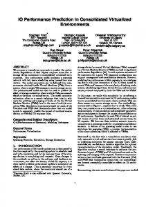
Flushing the dirty pages lazily is known to improve the performance of writes to a large extent. One of the important design issue however is to decide on when exactly to flush them. Traditional UNIX [38] systems do it periodically in which the dirty pages are written back when their age reaches a pre-defined limit. Some modern operating systems employ a slightly more sophisticated approach; when the number of dirty pages in the cache exceeds a certain threshold, a thread wakes up and starts flushing the dirty pages to the disk [56]. By this method, the page cache will always have sufficient free pages to allocate memory to satisfy new reads and writes. However, these policies suffer from a drawback in the form of lower disk utilization and adverse effect on other synchronous processes. This is because, the write-back is not fairly distributed along the time axes and they occur in bursts. For a write-intensive workload with intermittent synchronous requests, this problem will be more felt. The synchronous requests that at sent to the disk when the periodic background flushing takes place, it suffers undue latency. This problem is well motivated in a recent research [11] which proposes a method to adaptively schedule the flushing operation based on the read-write ratio of the workload. Figure 1 shows the effect of the background flushing operation in the access latency of foreground read requests. The spikes 19
Time (in ms)
10000
Access Time
1000 100 10 1 10
20
30 40 50 Request #
60
70
Figure 1: Read with Write in the access times are the instances when the background flushing occurs. Ideally, the background flushes should not delay the servicing of synchronous requests. When the flushing operation is done in a smaller granularity whenever the disk is idle, the overall dirty pages in the cache at any instance will be lesser. This can reduce the disk congestion during the periodic flushes and hence reduce the access latency of the synchronous requests. This scheme is more practical because disks are idle for significant fraction of time in many workloads. Especially for the write dominated workloads where the request reaches the disk only during the flushing instances and for CPU intensive workloads where between each disk requests there is a considerable CPU time spent(as in the case of large compilations) the disk is idle for a significant fraction of time. Hsu et.al in their paper ”Characteristics of I/O Traffic in Personal Computer and Server” presents a quantitative study on the various workloads in personal and server computers [39]. They have made their study at the physical level and they strongly argue that there is considerable amount of idle times in most of the common workloads and that they can be utilized for performing
20
Time (in 100 ms)
Disk Idle time for kernel compile 100 90 80 70 60 50 40 30 20 10
Idletime
0
500
1000 1500 2000 2500 3000 Timeline
Figure 2: Idle times background tasks like block re-organization. 3.1.2
Why Pro-active Disks?
Here we answer the question, why pro-active disks are a suitable infrastructure to implement the opportunistic flushing. The idea of writing back the dirty pages when the disk is idle is not entirely a new concept. Golding et.al [37] explored the benefits of running the background tasks whenever the disk is idle. In a single system, this can be easily done without the aid of a pro-active disk. The file system can accurately estimate the depth of the disk queue and hence the idle bandwidth of the disk at any instance based on the requests issued to the disk. But in the case of a multi-client environment, where a group of clients write to a single disk, the idle bandwidth of the disk cannot be estimated by any of the clients because one client does not know about the requests issued by the other client. The idleness detection can only be done by the disk because only the disk acting as a server will have the overall view of all the clients and the requests issued from all the clients.
21
3.1.3
Design
A pro-active disk continuously checks for idle bandwidth and when identifying one, pulls the small chunk of dirty pages from the file system cache. Detecting idleness: Determining the idle bandwidth of the disk accurately is a key design issue for this case study and the disk-state monitor is responsible for it. The disk queue depth can be one of the significant data structure to estimate the idleness of disk. When the depth of the disk queue falls below a certain threshold, we could assume that the rate of incoming requests to the disk is lesser and infer that the disk is idle. Similarly when the depth of the queue reaches a certain upper threshold, the disk can be deemed to be busy. This method of idleness detection is similar to the one described by Golding et.al [37], where he explores the various idle tasks that could be done when the disk is idle. Deciding on the lower and the upper threshold values for the disk queue depth is again a design issue. This can also be made to be adaptive based on the nature of the current workload and the history of success of past predictions. Another criteria that can be monitored to detect the idleness is the time of last request. If the time elapsed after a request exceeds a certain timeout, it may be assumed that no requests will be arriving to the disk for some more time in future. But for this method to work, the frequency at which the condition is checked and the granularity of the write-backs are important factors. To avoid false positives and the false negatives, the frequency of checking the idleness condition should be made very high and the granularity of the write-backs to be very low. The frequency of checking the idleness condition also depends on the granularity of the write-back. The frequency of the idleness condition should be at least as high as the time required to write-back the specified number of pages. For eg. if at every signal, 16 pages of data is to be written back to disk, and if we assume that this write-back takes 120 milliseconds to complete, the frequency at which the idleness condition is checked should at least be 120 milliseconds. Otherwise, the write-back itself would render the disk busy and the idleness checker would return failure. Number of pages to be written back: Once the idle disk bandwidth is identified, by 22
the disk-state monitor, the opportunity detector has to decide on the number of blocks to be obtained from the file system. This is important because, when a large number of blocks are requested from the file system, it would take more time to be serviced by the disk. As we cannot estimate accurately on how long the disk will be idle, there are chances of a synchronous request getting delayed because of this disk-induced flushing. Therefore, the number of blocks to be flushed for every signal can be kept very low and the frequency of sending signals to the file system can be kept very high. After the opportunity detector decides on the number of pages/blocks to be requested from the file system, the opportunity utilizer generates a PULL signal for those blocks and issues it to the file system. The file system on receiving the PULL signal, can write back the requested number of pages/blocks from its cache. 3.1.4
Implementation
The implementation of opportunistic flushing in our pro-active disk infrastructure involved adding a capability for idleness detection in the disk-state monitor and generation of an appropriate PULL signal in the opportunity utilizer module. The disk-state monitor spawns a separate thread is disk free for detecting the idleness of the disk. It wakes up every t ms and checks the current value of last request time and the queue depth The last request time is the time recorded at the time of the last request that arrived at the disk and it gets updated every time the disk gets a new request; thequeue depth is the current value of the depth of the disk queue and it gets updated on every insertions and deletions in the disk queue. Once the disk-state monitor records the values of last request time and queue depth it is sent to the opportunity detector. The opportunity detector compares these values with their respective threshold values that are already preset in the system. The value of the threshold for the time elapsed since the last request and the minimum depth of the device
23
queue can also be made to be adaptive based on the current nature of workloads and the history of past predictions. But in our implementation we hard-coded those values for the sake of simplicity. These values can be configured by changing the parameters WAKEUP FREQ and MIN DEPTH. If the value is greater than or equal to the threshold, the opportunity detector modules passes success to the opportunity utilizer. Otherwise the opportunity detector ignores the signal from the disk-state monitor. The opportunity utilizer, after receiving a success signal from the opportunity detector, generates a signal PULL(NULL, NUM BLKS). The field NUM BLKS tells the file system, the number of blocks to write back on receiving the signal. The first argument is NULL because, it is left to the file system’s page cache reclamation algorithm to choose the appropriate page to flush. This may be based on the age of the dirty pages present in the cache. Since the first argument is NULL, the page cache need not use the reverse mapping between the logical block numbers and the page addresses. It can just calculate the number of pages to flush based on the number of blocks that is requested by the pro-active disk. For this calculation, the file system just needs the size of the page and the size of the logical block. 3.1.5
Evaluation
In this section we present an evaluation of the proactive disk prototype with the capability of opportunistic data flushing. The experiments were conducted in a setup that is illustrated in the ”System setup” part of the section 2.3. We tested our prototype with a set of synthetic workloads, micro-benchmarks and real-world workloads. 3.1.5.1
Synthetic Workload
We generated a sequence of reads and writes from two different clients. One client iteratively read a random set of 50 blocks and induced a delay of 2 seconds in between and other client iteratively wrote 200 random blocks of data and induced a 3 second delay in between. For both the regular disk and the pro-active disk, we used the same sequence of 24
Table 1: Response Time of 50 block reads at discrete flushing intervals Request Number
12
Regular Disk
Proactive Disk
Response Time (ms)
Response Time (ms)
6478
344
24
6755
416
45
11483
1645
65
10543
1231
randomly ordered blocks for both read and write. Figure 3 shows the improvement in the read performance of proactive disk over the regular disk. The x-axis here shows the request instances and the y-axis shows the response time for reading 50 blocks of data. In the case of regular disks, the huge spikes at discrete time intervals signify the effect of the routine flushing of the dirty pages on the performance of the read requests. In this worst case, the time taken for reading 50 random blocks of data takes as high as around 10 seconds to complete. But in the case of the pro-active disk, we see that the spikes at those discrete intervals are considerably reduced and the maximum latency of the 50 reads in this case is 1.2 seconds. The values of the response time of reads at the discrete flushing intervals are tabulated in Table 1. This improvement is because, the dirty pages gets flushed in parts whenever the disk is idle and hence, at the discrete intervals where the routine file system flushing happens, the number of pages that need to be actually flushed is lesser. Therefore, the synchronous read operation is less affected during the time of routine flushing. Even during other time periods, there is no noticeable overhead in the read performance because of writing the dirty pages continuously whenever the disk is idle. This shows that our inference on the idle disk bandwidth is reasonably accurate. If there is some error in identifying the idle disk bandwidth, the dirty pages would be flushed even when the disk is busy responding to the synchronous reads and hence there would have been a raise in the read latency. Hence, this graph shows how our design improves the performance and also the accuracy of inferring the idle disk bandwidth.
25
Regular Disk Pro-active Disk
Time (in ms)
10000 1000 100 10 1 10
20
30 40 50 Request #
60
70
Figure 3: Response time of 50 block reads with background write 3.1.5.2
Real-life Workload
We chose to experiment the proactive disk for a real-life workload viz. kernel compile. We chose this because, kernel compilation involves reading the source file, delay caused by CPU processing, and also scanty writes to the disk. We compiled the 2.6.17 kernel with minimal functionalities in one of the clients and in the background, generated some write requests from the other client at regular intervals. We measured the total elapsed time, user time, which is the time spent by the CPU in user mode, the system time, which is the time spent by the CPU in kernel mode. Wait time is the elapsed time less the user time and system time. Therefore, wait time is the period during which the CPU is idle. This can be because of a blocking IO or because of waiting for a lock. Since it is a single thread environment, we assume the lock contention is negligible. We therefore regard the wait time as the IO time. As we expected, there is an improvement in the performance of compilation. We compared the overall completion time under proactive disk and a regular disk. Figure.4 shows a 3% improvement in the overall elapsed time in case of proactive disk. The improvement in the IO time is almost double in the case of proactive disk. A 26
Elapsed Time (seconds)
500
Wait User System
400 323.8
316.3
Regular
Proactive
300
200
100
0
Figure 4: Linux kernel compilation regular disk consumes an IO time of 26.35 seconds while a proactive disk consumes just 13.02 seconds which is a 51% improvement. This is because, in the case of proactive disk, the dirty pages are written back to the disk in its idle bandwidth. The kernel compilation generated the needed idle bandwidth in the disk whenever the CPU is busy compiling the source code. Therefore, when the dirty pages were written back during the idle time, the reads(of the source files) suffered lesser overhead during the routine flushing of the file system. But in the case of regular disk, most of the idle times generated by the kernel compile workload are wasted without performing any useful operations. During the routine flushing of the file system, the reads are more affected because of the congestion in the disk.
3.2 Intelligent Track-Prefetching We developed this application to illustrate the PUSH infrastructure of proactive disks. In this case study, we have developed a new approach to pre-fetching the blocks into the file
27
system cache. As opposed to traditional pre-fetching that is done by the file system, a proactive disk uses the access pattern information to decide on which blocks to pre-fetch to the file system cache. 3.2.1
Background
Disk media is comprised of tracks and sectors and the disk head moves at the granularity of sectors during rotation and at the granularity of tracks at the time of seek. Modern SCSI disks have a fast volatile memory embedded in them called the track buffers. These track buffers can store many tracks of data that encompasses the current working set. The track buffer capacity is usually very small when compared to the file system’s page cache. Even though they are small, they play a significant role in reducing the disk’s service time. The disk firmware uses certain simple heuristics to decide on when to pre-fetch the track data to the buffer. Usually, when a sector is accessed and when are are no other requests that are waiting to be serviced from other tracks, the track that holds the accessed sector is brought to the track buffer. The request is then serviced from the track buffer. When subsequent sectors from the same track is accessed, it will be serviced from the track buffer thus avoiding the disk seek time. The track buffer is thus very useful for workloads that are not purely sequential but encompasses a very small working set spanning a single track. However, the track buffer will not be useful in the case of random workloads encompassing a working set that is larger than the track that resides in the buffer and also in the case of purely sequential access because, the adjacent data will anyway be pre-fetched by the file system. The capacity of track buffers is generally small, they are reclaimed with new tracks frequently when the workload covers a larger working set. 3.2.2
Motivation
As the difference in speed continues to expand between the processor and the disk subsystem, the effect of the disk latency on the overall system performance is significant.
28
Prefetching–speculatively reading data on prediction of future requests–is one of the fundamental techniques to improve the effective system performance. However pre-fetching is useful mostly in the case of sequential accesses alone. Most policies turn off the prefetching logic when the sequential access is stopped. Prefetching data during random accesses can be detrimental to the system performance as they tend to waste the cache space with useless data. This may explain why despite considerable work [] on pre-fetching policies and enhancement, most general purpose operating systems still provide only sequential pre-fetching and other straight-forward variants of it. In most existing systems, the pre-fetching policy suffers from false positives and false negatives because, they detect the access patterns and issue read-ahead commands at the file system level. Therefore, they just rely on the logical block layout information while making the sequentiality decisions. But, as the disk system ages, many of its sectors can be re-mapped to different locations that the file system is unaware of. In those cases, the prediction made by the file system proves inadequate and results in disk seeks to random locations during read-ahead. Only the blocks that are physically and temporally adjacent to the current block should be pre-fetched. This motivates the need for leveraging the disk’s internal information for pre-fetching. Also, there may be certain workloads whose blocks that are temporally related but confine to a small working set and are not adjacent to each other physically. Existing approaches tend to ignore this kind of accesses when deciding on pre-fetching–they just consider purely sequential access. However, pre-fetching the entire working set in these cases can be improve the system performance. This can be very much requisite in a situation where there are two processes A and B and when A accesses discrete blocks in a small working set and B accesses a set of blocks that are very far from the blocks accessed by process A. In this case, if the entire (small)working set of process A has been pre-fetched, the disk head need not move back and forth for servicing the blocks of both A and B. This can improve the response time of both A and B. This problem is alleviated by the
29
presence of track buffers. However, the smaller size limits the utility of the track buffer. Even in modern disks of capacity 300 Gigabytes, the size of the track buffer is just 16 Megabytes. As most request to the disk passes through the track buffer, it gets frequently reclaimed. Consider two workloads running in parallel: one of them is purely sequential and it accesses a large chunk of data from the disk, and other workload is random within a small working set. In this case, as the sequential accesses occur faster than the random accesses, the track buffers will be filled with the sequentially data and get reclaimed very often. Therefore, when a block is accessed due to the other workload it may be eliminated from the track buffer before another block from the same track is accessed again. Figure 5 and 6 illustrates the change in the significance of track buffer for two different kinds of workloads. Plotted are the access times of reading a random block with and without the presence of sequential workload runs in parallel and Figure 6 shows the same in the absence of a background sequential read. When a background sequential workload runs, 2 out of 600 blocks are hit in the track buffer while 447 out of 600 blocks hit the track buffer in the absence of a background sequential workload. Since increasing the track buffer size doesn’t solve this problem completely, we propose to use a pro-active disk to leverage the bigger file system cache to store the reclaimed track buffer data. 3.2.3
Design
Disk-initiated Prefetching is a technique by which the pro-active disk tells the file system on what data to pre-fetch to its cache. The pro-active disk decides on the pre-fetch data by monitoring the access patterns in the on-disk track buffer. When a track in the buffer is going to be reclaimed, the pro-active disk makes an estimate on whether or not the data in the track will be accessed. The disk-state monitor component of the pro-active disk, checks for criterions for estimating the importance of a track.
30
100000 Access Time Time (in usec)
10000 1000 100 10 1 0
100
200 300 400 Request #
500
600
Figure 5: Track buffer hits(Reads alone) 1. The number of track buffer hits in the recent past. When there are large number of track buffer hits in the most recent time window, it means that the data that currently resides in the track buffer comprises a significant portion of the current working set. Therefore, the track that is to be reclaimed may also be accessed in the near future as it is a part of the current working set. Hence we check this condition for estimating the importance of the data in the particular track. 2. The number of hits the particular track(that is to be reclaimed) had during its stay in the track buffer. This is checked because, even though the track buffer hits are higher than the threshold, when the track that is to be reclaimed is not even accessed once, then it is not expected to be accessed in the near future and therefore, we do not choose that track for pre fetching. The workload monitor checks the access pattern as to whether or not it is sequential. The access pattern in the track buffer is considered to eliminate the chances of requesting
31
100000 Access Time Time (in usec)
10000 1000 100 10 1 0
100
200 300 400 Request #
500
600
Figure 6: Track buffer hits(Reads with background sequential write) the file system to pull a sequentially accessed track. This is because, in the case of sequential workloads, the data in the track(that is to be reclaimed) would have been pre-fetched by the file system already and it might reside in the page cache. Therefore, we restrain from sending wasteful signals to the file system. Another interesting design issue is deciding when to issue the PUSH signal to the file system. There are three options to do this: 1. When a new request to the disk warrants a reclamation in the track buffer, a PUSH signal can be generated for the track that is to be reclaimed and the request can be satisfied. However, this approach has a major drawback because, before the file system acts on the PUSH signal, the track may be reclaimed from the buffer. In this case, the subsequent file system read will be serviced by the disk and thus incur a large amount of extra overhead. 2. When a new request to the disk warrants a reclamation, the request can be blocked
32
and the signal can be sent to the file system to read the last track(that is to be reclaimed) in the track buffer. Once the file system reads the track, the old request can be serviced. This solves the above mentioned problem but will unnecessarily block the incoming request. 3. The method we promote is to have last few tracks in a bounded window and send the signals for those tracks in the window even before any request warrants a reclamation. By keeping the window reasonably big, the chances of reclaiming the track before the file system reads it can be avoided. At the same time, the other incoming requests need not be blocked during this period. The significance of the track data is estimated and the signal is sent only in the background. 3.2.4
Implementation
We implemented the PUSH infrastructure prototype of proactive disk, which performs track pushing. We maintain all the details about each track in the buffer inside the tr buffer desc structure. This has a field cache access counter that stores the number of times the track has been accessed during its stay in the track buffer. This value gets reset every time the track is removed from the buffer. To trap the sequential access patterns within a track, there is a field called last accessed blk. This stores the block number of the last requested block in that track. When the subsequent request to that track accesses the block adjacent to the block number stored in the last accessed blk, it is deemed to be a sequential access. The sequential access cannot be tracked by monitoring the requests to the whole buffer - we need a per-track data structure to monitor this. This is because, the sequential accesses may be interleaved with other accesses when reaching the disk. The time window is maintained as two discrete time values viz. initial time and current time. For every one second advancement in the current time, we increment the initial time by a second. A global value called
33
the track buffer hit ratio is calculated whenever a change occurs in the time window. This value tells the overall track buffer hit rate during the most recent time window. The tr buffer desc structure stores another flag in transfer window that tells whether the track exists in the transfer window. A configurable value called transfer window decides the length of the window. When a track gets discarded or read from the transfer window, the next available track in the track buffer is added to this window. As the tracks are added to this window, their significance for the current workload is checked and the file system is signaled. When a track is read from the window in full, there is no change in the LRU structure. The track is just discarded after the read completion. This avoids the movement of the track ahead in the LRU when the file system reads it ahead. The aforesaid values are compared with the preset threshold values. Based on the results of comparison, the significance of the track is estimated. When the track is estimated to be useful in the near future, make send ready(track number) is called. This function extracts the start block of the track and the length of the track from the tr buffer desc structure. Finally PUSH(block num, num blks) signal is issued to the file system. The block num is the start block of the track and NUM BLKS is the length of the track. The file system, on receiving the PUSH signal from the proactive disk, issues a read signal for those blocks(comprising the whole track) which are serviced from the track buffer of the pro-active disk. 3.2.5
Evaluation
In this section we present an evaluation of the pro-active disk prototype that has the capability of predicting and pushing, popular tracks of data. The experimental setup where similar to the setup discussed in ”system Setup” part of Section 2.3. We evaluated this case study with a commonly used micro-benchmark called IOzone [58] and a synthetic mix of OLTP-like small reads and OLAP-like large-scale batch reads.
34
Table 2: IOzone Benchmark showing throughput in KBps Regular Disk
Pro-active Disk
Size(in MB)
write
rewrite
read
reread
rand read
rand write
backward read
strided read
512
64633
48908
24580
24502
1294
10889
4233
4868
1024
53168
49394
27777
27567
905
37707
5582
4932
512
62641
49130
23487
25753
1431
14138
16213
17363
512
54614
40244
46937
27933
1010
38762
15916
16162
400
Wait User System
Elapsed Time (seconds)
350 300 250
226.7
200
178.3
150 100 50 0 Regular
Proactive
Figure 7: Response time for reading 5000 blocks 3.2.5.1
Experimental Setup
The experiments were performed on the following setup. The target ISCSI runs on a 2.4 GHz Intel Quad Processor with 4 Gigabytes of physical memory and it is connected with the ISCSI client through Gigabit Ethernet. The configuration of the client is a 2.26 GHz Intel Pentium IV Processor with 512 Megabytes of physical memory. The prototype of proactive disk that performs track pushing was done by modifying the simulation part of the ISCSI target code.
35
3.2.5.2
Workloads
(i) IOzone : We ran the IOzone workload for various file size ranging from 128 to 1024 Megabytes. IOzone performed various throughput measurements for read, write, rewrite, backward read, strided read, etc. In the background we ran a sequential workload continuously. We conducted the experiments for two file sizes 512 MB and 1 GB. The Table 2 shows the difference in the throughput measurements of the regular disk versus the proactive disk. From the table we see that there is lesser overhead in the performance of backward reads and the strided reads. In the case of backward read, the read starts from the end of the file and moves 2 blocks backward for every reads. In the regular disk, the throughput measured is 4.5 Kilobytes per second. Though the backward reads should have benefitted from the track buffers, because of the background sequential reads, the track buffer gets flushed so frequently that its benefit is not utilized. Therefore, almost all requests are satisfied by the disk with the inherent seek and rotational delays. But in the case of proactive disk, as we send the whole track data to the cache, many accesses get satisfied from the cache itself and therefore we see a significant improvement in the throughput. Similarly in the case of strided reads, we used a stride constant of 8*record size. Therefore, the reads happen in steps of 8 blocks. In this case, the proactive disk outperforms the regular disk by a significant portion. For other kinds of workload namely the write, rewrite and sequential read the throughput values of regular disk and the proactive disk look comparable. From these values, we find there is no significant overhead in employing the proactive approach of pushing the tracks. For random writes we see slight improvement in the throughput value. For a relatively smaller file of 512 MB, the improvement in proactive disk is more when compared to a larger file of 1024 MB. This is because, as the working set is smaller, there are more chances of the pushed track data to be accessed again. (ii) OLTP with background OLAP: We simulated a synthetic workload that runs similar to the real life workloads namely Online Transaction Processing(OLTP) and Online Analytical Processing(OLAP). We generated sequential read workload on a large file and ran a 36
Access Time
Access Time
10000 Time (in usec)
Time (in usec)
10000 1000 100 10
1000 100 10
1
1 1K
2K 3K Request #
4K
5K
1K
(a) Regular Disk
2K 3K Request #
4K
5K
(b) Proactive Disk
Figure 8: Per-block response time for OLTP random workload on a small file. This is analogous to running OLTP workload when some analytical processing is done in the background. The sequential workload ran continuously and the other read workload performed read on 5000 random blocks within a small working set of 100 Megabytes. We also introduced a 1 second delay for every 50 block reads. We measured the time taken for completion and the cache hit ratio for reading these 5000 blocks and plotted a graph. Figure.7 shows the performance improvement of a proactive disk over regular disk. This graph plots the elapsed time, the user time and the system time for reading the 5000 blocks of data. From the graph we see that the wait time, which is the elapsed time less the user time and the system time, is lesser for proactive disk, when compared to the wait time of the regular disk. This is because, in the case of regular disk, the blocks are not pre-fetched by the file system because of the random workload. When a block is accessed, the whole track is transferred to the track buffer. However, as there is a sequential read progressing in the background, the track buffers are reclaimed very often. Therefore most of the read request goes to the disk. In the case of proactive disk, When the tracks are sent to the file system cache. Therefore, when another random block in the same track is accessed, it will be hit in the file system cache. This is the reason for the considerable improvement in the IO time of proactive disk. Figure.8 and Figure.9 shows the performance improvement in a different perspective. The individual response time of the blocks are plotted as a function of time. As in the graph, most of the requests gets
37
serviced by the regular disk. In the case of proactive disk, we find that more than 55% of the requests are serviced by the file system cache as against the 1% cache hit for a regular disk.
3.3 Related Work Opportunistic Flushing : The drawbacks of adopting naive periodic update policy adopted by most commodity operating systems were studied in past research projects. Carson and Setia [18] showed that for many workloads the naive periodic update policy perform worse than write-through caching. Mogul [56] proposed a policy by which the age of individual dirty pages are taken into account for deciding the flushing interval. Golding et al [37] described a technique of flushing the dirty blocks during disk idle times. This is similar to our approach, but differs usage scope and technique used to find disk idle bandwidth. The main advantage of our approach is, since the idle bandwidth is extracted at the disk level, it is bound to be more accurate and it can be deployed for more than one clients. Recently Batsakis et al [11] proposed a de-staging policy that considers the memory allocation ratio for write buffering and read caching. Wise ordering of Writes [36] project proposed a destaging policy that uses both the temporal and spatial locality information to decide on the flush timing and the flush data. Disk-predicted Prefetching : Recently, Ding et al [31] have studied the importance of exploiting the disk layout information while making pre-fetch decisions. They propose a method to monitor the access history information and the block-level correlations at the logical block level and use those information for making pre-fetch decisions. The idea of shifting the data across layers of a multi-level cache system has been studied in the past in both upward and downward directions. Wong et al [84] proposed demote interface to transfer the data reclaimed from file system cache to the disk cache and recently, Gill et al [35] explored the promote interface to transfer the data from disk cache to the file system cache. Researchers have also explored the options of utilizing the application hints to make
38
pre-fetching decisions [61].
39
CHAPTER IV
STORAGE CHALLENGES IN VIRTUAL ENVIRONMENTS
The cloud computing paradigm is the backbone of various Internet services that take an ever increasing fraction of time people spend on computers today. By hosting data and applications in a server farm (i.e. a data center) and providing access through a thin-client, such services/applications enable ubiquitous access to data besides the ability to harness massive computing power even from portable devices. Cloud computing allows customers to only pay for the computing resources they need, when they need them. In order to enable support such cloud-based applications in a cost-effective manner and to lower the barrier to entry for such applications, a somewhat recent business model that has emerged is that of a service provider hosting third-party applications in a shared data center (e.g. Amazon’s EC2 platform). A key technology that enables such cost-efficient resource sharing in such data centers is virtualization; by providing isolation and separate protection domains for multiple third party applications, virtual machines [43, 10] enable server consolidation, and consequently significant savings in the cost of managing such data centers. Unfortunately, one complexity that arises with virtualization is that it becomes harder to provide performance guarantees and to reason about a particular application’s performance, because the performance of an application hosted on a VM is now a function of applications running in other VMs hosted on the same physical machine. Also, it may be challenging to harness the full performance of the underlying hardware, given the additional layers of indirection in virtualized resource management. While many virtual machine platforms provide good CPU isolation and minimal CPU overheads [43, 10], we find that when it comes to I/O performance, virtual machines result in some interesting and non-obvious
40
interactions and side-effects. In this chapter, we present a detailed experimental analysis of the I/O performance observed in a virtualized environment. Through a series of systematic experiments on the Xen [10] VMM platform, we show that the storage I/O performance observed by an application inside a VM depends on various aspects such as which disk partition the virtual machine uses, the CPU utilization of other VMs on that system, the nature of I/O performed by other VMs on the hosted system and the block size used for performing disk I/O. In many cases, the performance difference between the best choice and the average (eg. default) choice is as high as 8% to 35%. We also evaluate the costs of using a virtualized environment compared to a dedicated physical system, in terms of I/O performance.
4.1 Background In this section we present some background on general concepts of cloud computing and the role of virtualization on cloud. Cloud Computing can be perceived in two layers namely the applications that are delivered to clients as a service over the Internet and the hardware and software in the datacenters that provide those services. The hardware resources in the data-center is often referred as the ‘Cloud’. There are at least three major categories of Cloud viz. the compute cloud, infrastructure cloud and internal cloud on the basis of their usage model. Compute Cloud runs applications for clients and can be accessed by the client as a service. Examples for this type of cloud is Google Docs, Google AppEngine, etc., Word processing application is run in Google’s cloud and customers access the applications as a service. Infrastructure cloud has a slightly different business model and customer base. These are large installations of servers that are usually virtualized, and each individual virtual machines serve the customers. By design, these are configured dynamically based on the user’s requirements. One of the most common example for infrastructure cloud is Amazon
41
Elastic Compute Cloud (EC2). Customers have the option to purchase a specific configuration of resources from the cloud for a specific amount of time. This type of cloud setting has gained tremendous importance in the recent past and one of the fastest growing business model mainly because of the flexibility it offers. For eg. if a user wants to run a large-scale simulation that takes 1000 hours on a single server, he has the flexibility to run the same simulation in 1000 servers for 1 hour at fairly the same cost [9] if the application provides such levels of parallelism. Internal Clouds or Private Clouds are computing resources aggregated to server internal business activities and are not available to the general public. In this chapter, we focus on performance issues in an infrastructure cloud setting. One of the most significant functionality offered by infrastructure cloud is the ability to configure different scale of resources dynamically based on the requirements. System virtualization is one the basic foundations that makes such flexibility of resource provisioning feasible. Typically, whenever a user purchases a specific set of resources in specific configurations, he gets a virtual machine that uses underlying physical resources from one or more nodes. The user perceives it as a separate physical machine and expects peak performance at all times. However, this is typically not the case because various virtual machines from different users may share a physical resource leading to resource interferences. Also, there is inherent performance issues in using a virtual machine when compared to the physical machine as shown in our experiments. It is therefore important to understand the effects of these interferences and overhead to propose ways for optimal performance.
4.2 Measurements In this section we present our empirical results in four groups based on their impact on the cloud service providers, application developers and the customers. We start with presenting results that provide insights on how to provision and place virtual storage space in physical devices. We then present the effects of workload interactions across multiple VMs that use
42
a shared physical resource. We finally provide results showing the performance impact of I/O block sizes for different workloads some of the differences between using a physical machine versus a VM. 4.2.1
Experimental Setup
We conducted all our experiments on a 2.4GHz Intel Quad-core machine with 4 GB RAM and two Seagate 7400 RPM SATA hard disks of 250 GB each. We used Xen hypervisor [10], version 3.3.1 and created two guest domains Dom1 and Dom2 . We used physical disk volumes for every partitions in each of the guest domains by default. We used a variety of monitoring tools such as Xenmon [22], Xentop, iostat, blktrace and btt. In cases where we record the block-level trace using UNIX blktrace utility, we used separate physical disks for recording the trace − this avoids most of the disk-level interference caused by the tracing activity. Each of the guest domains were allocated a single dedicated processor core as it reflects typical enterprise setting. Depending on the nature of experiments, we varied the guest domains’ RAM size from 128MB to 1GB each. 4.2.2
Physical Machines vs. Virtual Machines
The Pros and Cons of using a virtual machine: Our first set of experiments are aimed at identifying additional overhead introduced by using a virtual machine when compared to its physical machine equivalent for different types of I/O workloads. For these experiments we carefully configure the VM and the physical machine resources such that the comparison is fair. In addition to using the same amount of hardware resources, we used the same operating system (Ubuntu 8.04 Server), kernel version and the I/O scheduler in both cases. We used CFQ (Completely Fair Queued) scheduler for both physical machine and Dom0 . The guest domains’ I/O scheduler is set to ‘noop’ so that they do not schedule the requests themselves before they are queued in Dom0 . First, we run Postmark benchmark on both physical machine and its equivalent virtual machine and record the bandwidth achieved in both cases. Figure 11(a) shows the 43
1000
1000 Read-256M Read-512M Write-256M Write-512M
10
Read-256M Read-512M Write-256M Write-512M
100 Latency in ms
Latency in ms
100
1 0.1 0.01
10 1 0.1 0.01
0.001
0.001 0
10000 20000 30000 40000 50000
0
Requests sorted by their Latency
10000 20000 30000 40000 50000 Requests sorted by their Latency
(a) Physical Machine
(b) Virtual Machine
Figure 9: Latency : Physical machine vs. Virtual machine
40 Physical Machine Virtual Machine
Cache Hit Rate (%)
35 30 25 20 15 10 5 0 256
512 1024 Cache Size (in MB)
Figure 10: Cache Hit Rate - Physical Machine vs. Virtual Machine
bandwidth measurements (MB/sec) of postmark benchmark under various file sizes. The bandwidth achieved by the physical machine is not much different from that of the VM for small file sizes (1KB, 10KB). As the file size increases there is increasing drop in bandwidth in virtual machine bandwidth, when compared to physical machine bandwidth. This is because, when the file size is small and when they are spread across many directories, the Postmark transactions are seen by the disk as random accesses. As the file size increases, the accesses become more and more sequential. Therefore, the overhead induced by virtualization is amortized by the disk seek overhead in the case of small file sizes. As the file size grows, the disk seek overhead is reduced, thus projecting the virtualization overhead. In order to understand the virtualization overhead in the case of large file size (or sequential access), we picked up a constant file size of 10MB and ran the Postmark benchmark with varying block sizes. Figure 11(b) shows the bandwidth of Postmark workload
44
running in a physical machine versus a VM. As the block size reaches 1MB, the virtual machine achieves performance similar to that of a physical machine. This is because, a small and fixed overhead is introduced in the virtual machine for every system calls/requests. This can be attributed to the extra layers introduced by virtualization technique. Therefore as the block size increases, the same amount of work is done by issuing lesser number of requests, thus reducing virtualization overhead. Figure 4.2.2 shows performance of postmark benchmark with 10MB file size, when two instances of the benchmark are running in two VMs simultaneously. We compare the performance of running two instances in a single disk versus running them on two different disks for both physical machine and virtual machine. Overall we observe that there is a 32% difference in bandwidth between physical machine and its virtual machine equivalent both in the case of single disk and two separate disks. Next, we show that virtual machine performs better than a physical machine in some specific cases resulting from an inherent design advantage of virtualization technology called Cache Isolation. In a physical machine, the cache space is generally not partitioned equally across processes because one process may use the cache space better than the other. On the flip-side, there is a chance that one process may be unduly affected by another process, such as when the other process uses the cache aggressively than the other. For example, when there are two processes, one doing large amount of writes and other process reading a set of files frequently, the cache space may be aggressively filled by the write process leaving no space for read cache. This is not the case for two VMs because the cache space is well divided between the two VMs. Therefore it is beneficial to run two workloads competing for cache space in two different VMs than on a single VM or a single physical host. We confirm this hypothesis by conducting a set of experiments that capture the latency, cache hit rate and overall bandwidth. For these experiments, we run synthetic read workload that models Zipf distribution of accesses in the foreground and run a background sequential write workload. We tailored our foreground workload such that
45
40
90 Physical Machine Virtual Machine
80 Bandwidth in MB/s
Bandwidth in MB/s
35 30 25 20 15 10 5
70 60 50 40 30
Physical Machine Virtual Machine
20
0 1K
10K 100K 1M File Size (in Bytes)
10M
4
(a) Bandwidth wrt. file size
8
16 32 64 128 256 1K 2K Block Size in KB
(b) Bandwidth wrt. block size
Figure 11: Bandwidth: Physical Machine vs. Virtual Machine
the blocks are generally accessed randomly and 20% of the blocks are accessed 80% of the time. Cache size of ‘x’ MB refers to ‘x’ MB of memory in the case of physical machine and partitioned as ‘x/2’ MB of memory in each of the two VMs. Figures 9(a) and 9(b) show the CDF of latency values of foreground read for two different cache sizes. The latency CDF of physical machine shows a sudden spike in latency(cache miss) at around 9% of requests for 256MB cache and around 22% of requests for 512MB cache size. This shows that the write workload consumes undue amount of cache space leaving lesser space for the foreground read workload. When this is compared to the performance in virtual machine setup, where even for aggregate cache size of 256 MB, around 19.5% of requests are hit in cache. The footprint of our read workload is 150 MB and background write workload is 400 MB. Therefore at 512MB of cache, the workload achieves top performance −any more increase in cache size no longer have any effect on the overall performance. For cache size of 512MB, both the read and write workload reside in the cache without affecting each other. Figure 4.2.2 shows precise cache hit rate for different cache sizes. These results show that virtualization provides better cache isolation between two processes running in two separate virtual machines, when compared to running them in a single physical system. Choosing right block size for the right workload: In this group of experiments, we analyze the significance of I/O block size of VMs on the overall I/O performance of the system. In our experiments we run synthetically generated random workload of varying 46
40 Bandwidth in MB/s
35
Instance 1 Instance 2
30 25 20 15 10 5 0 Phy-1disk VM-1disk Phy-2disk VM-2disk Configuration
200000 180000 160000 140000 120000 100000 80000 60000 40000 20000 0
45 No Locality Locality_4 Locality_8 Locality_16 Locality_32
40 Cache Hit rate (%)
Total Time Taken(ms)
Figure 12: Bandwidth wrt. no. of disks
35 30
No Locality Locality_4 Locality_8 Locality_16 Locality_32
25 20 15 10 5
4
8
16 32 64 128 256 I/O Size (in KB)
4
(a) Latency
8
16 32 64 128 256 I/O Size (in KB)
(b) Cache Hit Rate
Figure 13: Effect of I/O size on Performance
spatial locality between accesses. Our policy of defining the locality factor is as follows: Once a block is read, it is likely that ‘x’ more blocks out of the next ‘y’ contiguous blocks are read in the near future. In all experiments, the total amount of data read is configured to be the same. We read 16,000 blocks of data from a 1GB file. In ‘No Locality’, we read 16,000 blocks of data randomly, each 4KB in size. The remaining four cases, denoted as ‘Locality x’, represent the workload where we have a set of random accesses and between every such access, there are ‘x’ more block accesses within the neighboring 256 blocks. Figure 13(a) shows the difference in total time taken by the workload with respect to varying I/O block sizes for different locality factors. Clearly, as the block size increases, we see that the time taken for workloads with spatial locality constantly decreases. However, when there is no locality in the workload, the total time taken raises sharply as the block
47
size increases. Throughput showed similar behavior for block sizes ranging from 4KB to 256KB. The requests served per second increases for workloads with locality. This is because, when there is spatial locality in the workload, reading a large amount of data in one request helps in placing more data in page cache and future requests to neighboring blocks are served from the page cache. However, when the block size is small, even requests to neighboring blocks are treated as individual random requests, thus reducing performance. When there is no locality of data, reading in larger block sizes reduces the performance because irrelevant data are read into the page cache, leading to cache pollution and wasteful I/O bandwidth. Remarks: In our final set of experiments we derive two observations which will be useful for cloud customers and service providers: (i) Virtualization overhead is more felt in sequential workloads accessed through smaller block sizes than random workloads. The cloud customers can estimate the expected performance based on the characteristics of the workload they deploy. (ii) Cloud service providers can practice static partitioning of memory across multiple VMs hosted in a single physical machine, whenever strict performance isolation is important across different customers. 4.2.3
Virtual Disk Provisioning and Placement
Choosing the right location at the right disk: We then focus on identifying the impact of provisioning and placement policies for virtual disks on the overall I/O performance. In our experiment we have a single virtual machine running on a physical host. We test the performance of ‘Postmark’ benchmark [44] with a file size of 5KB in two different virtual disk size settings viz. 4GB and 40GB. Postmark benchmark is reminiscent of mail server workload with various configurable parameters like file size, block size, read/write ratio, etc., The 4GB and 40GB virtual disks are separate partitions from a single physical disk of size 250GB. The total data footprint of our workload is 150 MB, and the total number of files is 30000 spread across 500 subdirectories. As the file placement policy aims
48
300
300 Single Disk Request Disk Offset (in GB)
Disk Offset (in GB)
Single Disk Request 250
200
150
100
200
150
100 0
5
10 15 Time (in Seconds)
20
25
0
(a) Data Spread in 4GB Disk
5
10 15 20 25 30 Time (in Seconds)
35
40
(b) Data Spread in 40GB Disk
3
3 Throughput Average Throughput
2.5
Throughput (MB/S)
Throughput (MB/S)
250
2 1.5 1 0.5 0
Throughput Average Throughput
2.5 2 1.5 1 0.5 0
0
5
10
15 20 25 30 Time (Seconds)
35
40
0
(c) Throughput 40GB Disk
5
10 15 Time (Seconds)
20
25
(d) Throughput 4GB Disk
Figure 14: Provisioning of Virtual Disks to co-locate the files within only a single directory, the files from 500 subdirectories are spread across the entire virtual disk by the file system. Figure 14(a) and Figure 14(b) show the distribution of read accesses in both cases. We used Linux blktrace utility to collect the block level traces and plotted them in the context of the entire physical disk. When the virtual disk size is 4GB, the data (and hence the accesses) is confined to the 4GB(∼141GB145GB) space. However when the virtual disk size is 40GB, even a small data footprint of 150MB is spread across the entire 40GB(∼196GB-236GB) space. Figure 14(d) and Figure 14(c) show the corresponding throughput profile of each virtual disk respectively. The disk I/O throughput for 4GB setting is at 2.1 MS/sec on average, whereas for 40GB, it is about 60% lesser on 1.3 MB/sec. As the disk seek distance is vastly reduced when the virtual disk size is small, the throughput achieved by a 4GB virtual disk is significantly better than that of a 40GB disk for the exactly same workload. When disproportionate amount of disk space, with respect to data footprint of the workload, is allocated for a user,
49
20
File-backed Outer Zone Mid Zone Inner Zone
15 10 5 0 1K
10K 100K 1M File Size (in Bytes)
18
Avg. Response time Avg. Seek Distance
17 16
20 15 14
10
13 12 O-I
10M
30
O-M
M-I
M-M
Virtual Disk Placement
(a) Virtual Disk Placement
Average Seek Distance (Million sectors)
Average Response Time (in ms)
Bandwidth in MB/s
25
(b) Multiple Virtual Disk Placement
Figure 15: Placement of Virtual Disks some file system allocation policies or application decisions might lead to data being spread across a larger footprint on disk. Next, we present some insights regarding placement of virtual disks in a physical storage system. In the set of experiments reported in this paper we consider different cases within a single disk. However, the principles discussed here are applicable to large scale storage arrays as well. We start with the configuration of one VM per host and then extend to multiple VMs per host. The goal of these experiments is to identify the impact of placement of virtual disks on both the I/O performance of each virtual machine and the overall throughput achieved by the physical disk device. We consider four cases: (i) a file-backed virtual disk (which is common in most desktop virtualization setting), where a large file is created in the host’s file system and it is mounted as a disk in the virtual machine, and then virtual disks backed by physical partitions which are located in (ii) outer, (iii) middle (mid) and (iv) inner zones of a disk. We ran Postmark benchmark with varying file sizes in each of these settings and collected the storage I/O bandwidth values. Figure 15(a) shows the bandwidth achieved by each of these virtual disk configurations. We observe that the file-backed disk performs consistently worse than the other cases. This is because the virtual disk is essentially a file in the host file system and every time a virtual machine accesses its disk, the meta data for that file in the host file system need to be accessed as well. Therefore, meta-data access is doubled for most of the disk accesses by the virtual
50
machine − one within the virtual machine, and the other by the host file system. We also observe that, although there is not much variation across different configurations for small file sizes, the performance varies significantly as the file size increases. This is because as the file size gets larger, the sequentiality is increased and the subtle differences between various regions within the disk are clearly shown. In contrast, for smaller files, the accesses are mostly random and the disk seek overhead amortizes smaller differences in accessing various disk regions. In addition, we observe that for large files (sequential accesses), the performance is best when the virtual disk is placed in the outer-most zone. This is because the outer-most zones have larger tracks and sequential accesses benefit from a single large track read. As we move to the inner zones, the track size decreases and the sequential accesses would incur more and more track switches, reducing the I/O performance. Next, we try to understand the case of more than one virtual disks per physical host. The virtual disks may either be from a single VM or multiple VMs. We compare different cases of placing the two virtual disks and identify the best setting with respect to overall I/O performance. Figure 15(b) shows the average response time of Postmark benchmark with file size averaging to 10KB. We bypassed the file system cache in order to understand isolated disk behavior for different configurations by using ‘O DIRECT’ flag for the Postmark transactions. The six different configurations, with respect to placement of the two virtual disks, are: (i) One virtual disk in outer zone(smaller LBNs) and other in inner zone(larger LBNs)(O-I), (ii) One virtual disk in inner zone and other in middle zone(M-I), (iii) one virtual disk in middle zone and other in outer zone(O-M), (iv) both virtual disks in middle zone(M-M), (v) both virtual disks in inner zone, and (vi) both virtual disks in outer zone. We show the first four cases in our results as the other two results resemble the (MM) configuration. The secondary Y-axis shows the average seek distance of the requests reaching the physical disk. This value is obtained by running blktrace utility in the physical disk device. This result shows that when the two virtual disks are co-located, they provide the best performance when compared to other placement combinations. This is because the
51
seek-distance is reduced when the virtual disks are collocated, leading to faster seeks. Remarks: These experimental results deliver four important observations: (i) Cloud service providers can improve their storage efficiency by practicing thin provisioning of their storage resources. (ii) Customers of cloud storage can purchase storage based on their expected workload footprint rather than just the price. This is important because, customers may tend to purchase more disk space than what they need, especially when the price differential is not significant. (iii) It is beneficial to place sequentially accessed virtual disk in the outer zone of the disk to achieve better performance (Eg. VMs that host movies, large OS distributions, etc.,). (iv) When a cloud service provider needs to place multiple virtual disks in a single physical storage, those virtual disks whose accesses are temporally dependent on each other should be co-located for best performance. By temporal dependency, we refer to the cases where each of the two virtual disks are owned by one or more VMs such that the applications running on them are closely related or causally dependent on each other in the sense that both applications might issue disk requests fairly simultaneously. 4.2.4
Inter-VM Workload Interference
Choosing right workload for the right VM : Our final set of experiments are focused on understanding the interactions between different types of workloads running in multiple VMs hosted on a single physical machine. It is important to study such interactions because these are common cases in a typical infrastructure cloud setting, where VMs hosted in a physical machine serves to different customers. Therefore, it is important that a specific load from one VM should not adversely affect other applications running on other VMs hosted in the same physical machine. We dedicate this group of experiments to the understanding of two types of contention, as both affects the overall I/O performance: (i) one VM running CPU intensive application
52
Table 3: Effect of Dynamic Frequency Scaling on I/O Performance Freq. Governor Reqs/s Blks/s CPU Util CPU Freq(MHz) Idle CPU 4756 38042.5 64.7 1400 ‘Ondemand’ Busy CPU 5169 41344.8 63.8 2400 Idle CPU 5166 41314.2 62.9 2400 ‘Performance’ Busy CPU 5163 41302 63.2 2400 and another VM running disk intensive application; and (ii) both VMs running disk intensive applications. We first run a CPU intensive workload (a batch of floating point operations in loop) and a disk intensive workload (Postmark benchmark) in two different VMs, Dom1 and Dom2 , and track the performance of the disk workload in Dom2 . Intuitively, one might expect a drop in performance of the I/O workload when there is another VM running a CPU intensive workload, given that the Dom0 CPU is time-shared between all the domains. However our results show a different phenomenon. Figure 16(a) shows bandwidth achieved by Postmark benchmark with varying file sizes under two cases: (1) Dom1 is idle and Dom2 runs postmark benchmark, and (2) Dom1 runs CPU intensive task and Dom2 runs postmark benchmark. Counter-intuitively, the Dom2 I/O performance in case-2 is better than that of case-1. We initially suspected it to be Xen’s VM scheduling anomaly. We repeated the same experiments under a different Xen scheduler, namely SEDF, instead of using the default CREDIT scheduler. However, the results did not change significantly. In order to isolate this behavior with respect to workloads, we chose synthetically generated purely sequential workload. Figure 16(b) shows similar behavior across different CPU weight assignments for purely sequential file read. The ratio in the X-axis represents the weight ratio of virtual CPUs of the two VMs, Dom1 and Dom2 . We conjecture that this behavior is observed for sequential workloads across different Xen schedulers. We further investigated the experiments by a Xen monitoring tool-Xenmon [22] and recorded the ‘CPU Cycles/Execution’ metric, which shows the number of CPU cycles spent for a particular execution unit. Figure 4.2.4 shows the CPU cycles/Execution for both case (1) and case (2). We observe that case (1), where the Dom1 is idle, incurs more cycles per
53
25
34
Idle CPU in VM1 Busy CPU in VM1 Throughput (MB/s)
Bandwidth (in MB/s)
30
20 15 10 5
Idle CPU in VM1 Busy CPU in VM1
32 30 28 26 24 22
0
20 1K
10K 100K 1M File Size(in Bytes)
10M
1:1 2:1 3:1 4:1 5:1 CPU Allocation[VM1:VM2]
(a) Postmark Bandwidth
(b) Sequential Bandwidth
CPU Cycles/Execution
Figure 16: Resource Contention [CPU vs. DISK]
88000 86000 84000 82000 80000 78000 76000 74000 72000 70000 68000 66000
Idle CPU in VM1 Busy CPU in VM1
0
5
10
15 20 25 30 Time (Seconds)
35
40
Figure 17: Variation in CPU Cycles
execution than case (2), where Dom1 is running a CPU intensive task. We eventually found that this behavior is because of a power optimization technique used in the CPU, called Dynamic Frequency Scaling. It is a technique where the frequency of the CPU (and hence the power consumed) is increased or decreased dynamically based on CPU load. For an Intel Quad-Core processor and Linux kernel version 2.6.18, the dynamic frequency scaling is enabled by default. However, this policy is configurable by means of choosing CPU frequency scaling ‘governors’ in the Linux kernel, and the options available in Linux kernel are performance, powersave, ondemand and Conservative. Linux allows the user to set a particular CPU frequency scaling policy based on the power and performance requirements. ‘ondemand’ is the default option in Linux kernel 2.6.18, which means the CPU frequency is scaled dynamically based on load. The ‘performance’ option
54
is used to run the CPU at high frequency always and the ‘powersave’ option runs the CPU in lowest frequency always. The ‘conservative’ is similar to ondemand with slightly more bias towards either performance or power. Therefore, the fact that Dom2 I/O performance in case (2) (busy CPU in Dom1 ) out-performs that of case (1) (idle CPU in Dom1 ) is annotative: when CPU is idle in Dom1 , the overall CPU load on the physical host is less with just the I/O workload in Dom2 . Therefore the CPU is ‘under-clocked’ i.e., the CPU frequency is reduced, this results in the Postmark benchmark running in a lower frequency. When Dom1 runs a CPU intensive task, the overall CPU load is increased significantly, thereby switching the CPU to highest frequency automatically, thanks to dynamic frequency scaling. Though we have allocated separate cores to each of the VMs, the frequency scaling policy is applied to all cores equally. Therefore, the difference between case (1) and case (2) essentially represents the performance difference between the case when Dom2 CPU runs in highest frequency and the case when Dom2 CPU runs in lower frequency. In Figure 16(a) the dynamic frequency scaling phenomenon is less significant for smaller file sizes because random accesses on disk lead to larger seek delays, which amortizes delays due to reduced CPU frequency. Table 3 shows the throughput and CPU utilization values for the default ‘Ondemand’ policy and the ‘Performance’ policy along with the corresponding CPU frequency values. This set of results further testifies our measurement analysis. We next measure the effect of running two I/O intensive workloads on multiple VMs hosted on a single physical machine. For these experiments, we use Postmark benchmark and synthetically generated combinations of sequential and random reads. Figure 18(a) shows the achieved bandwidth of postmark benchmark for various file sizes in three different configurations viz. (i) one instance of postmark in a single VM and other VM remains idle, (ii) two VMs each run one instance of postmark and their virtual disks reside in same physical disk, and (iii) two VMs each run one instance of postmark and their virtual disks reside in different physical disks. We observe that case (ii) performs the worst among all three configurations as the sequentiality in both Postmark instances is affected when both
55
35 Time Taken (in sec)
Bandwidth in MB/s
30
60 1 Instance 2 Instances in 1 Physical Disk 2 Instances in 2 Physical Disks
25 20 15 10 5
VM 1 VM 2 Ideal
50 40 30 20 10 0
0 1K
10K 100K 1M File Size (Bytes)
10M
CFQ AnticipatoryDeadline Noop I/O Scheduling Policy
(a) Disk Contention
(b) Effect of I/O scheduler
Figure 18: Resource Contention [Disk vs. DISK]
% difference in time taken
30 Overhead
25 20
17.52
15 10 5
0.6
0.5
0.9
0 -5 -10 Seq(Seq) Seq(Rand)Rand(Seq)Rand(Rand) Workload Combination
Figure 19: Mixed Workload Performance
virtual disks(which reside in a single physical disk) are accessed alternatively. Interestingly there is roughly 24% difference in bandwidth for 10MB file size between cases (i) and (iii) even though each of the two VMs in case (iii) is running its virtual disks in separate physical disks (and with separate processor cores). This can be viewed as a scheduling overhead between the two virtual machines. As all I/O requests go through Dom′0 s block device driver, when one of the VMs is scheduled, the requests in the other VM waits for their turn and its disk might skip the sector to be read. This may lead to rotational delays even in the case of pure sequential workloads, hence accounting for the reduced bandwidth. In order to understand the effect of different I/O schedulers in Dom0 on I/O Performance in guest domains, we run synthetically generated sequential workloads in each of the two VMs whose virtual disks reside in two different physical disks. Figure 18(b) shows
56
the time taken for reading 100,000 blocks of data from a large file sequentially in the granularity of 4KB blocks. The ‘ideal’ bandwidth shown in Figure 18(b) is the bandwidth recorded when a single process reads 200,000 blocks of data. The comparison against this ideal bandwidth value shows the scheduling overhead when running two virtual machines, each serving half of this amount of requests. Figure 18(b) shows that the Deadline scheduler and the Noop scheduler(no scheduling) perform slightly better than the Completely Fair Queued scheduler (CFQ) for this particular workload. However, we observe that the performance does not change significantly across scheduling policies and the perceived overhead is inherent when alternating I/Os between multiple virtual machines. Figure 4.2.4 shows the performance overhead when running different types of I/O workload in difference combinations. We consider sequential and random reads and study four combinations of them. Every x-axis points is in the form foreground(background). For example, Seq(Rand) represents the performance overhead suffered by a foreground sequential workload when a background random workload runs simultaneously. The y-axis represents the percentage difference in time compared to running just the corresponding foreground workload (without any background workloads). We observe that when two sequential workloads run simultaneously, there is close to 18% performance difference compared to running a single sequential workload. Note that the foreground and background workloads are sent to different physical disks since we set up each VM with its own physical disk in this set of experiments. However, other combinations of sequential and random workloads induce very less overhead. This is because of the contention in one of the Dom0 ’s queue structures: two sequential workloads would populate the queue faster when compared to other workloads and therefore some of the sequential requests would have to wait before entering the queue. Remarks: Through this group of experiments, we make three observations, which are useful for both cloud service providers and their consumers. (i) Most of the infrastructure
57
cloud systems employ Dynamic Frequency Scaling technique to conserve power. Therefore, strategies for co-locating workloads can be critical for achieving maximum performance and at the same time conserving power. (ii) Cloud service providers should avoid co-locating VMs with two sequential I/O workloads on a single physical machine, even when each of them goes to separate physical disks.
4.3 Related Work In this section we provide some of the earlier work on virtual machine I/O performance study. The case of optimized performance in virtual environments has been studied in the past and most of them focus on sharing and scheduling of CPU [23, 78, 24], partitioning and sharing memory [82, 70], and networking [19, 59, 51]. However, IO optimization in the storage layer [77, 3, 29] has relatively been studied less. Most of these focus on effect of disk I/O on CPU [23] or effect of workloads on disk performance in virtual machine [3] or on I/O scheduling issues and impact of different scheduling policies on the I/O performance [29]. Nevertheless, there are no papers that study the interference of multiple virtual machines purely in the disk layer to the best of our knowledge. Provisioning and placement issues in enterprise storage servers have been studied in the past [4, 6] which is useful for large scale storage providers. But our experiments target the customers of cloud storage also in providing them insights into how much space they need to purchase for their typical usage. Researchers have presented the effect of CPU and the I/O performance in the perspective of CPU scheduling [23, 24], but the side-impacts of CPU power optimization policies on the I/O performance have not been studied before.
58
CHAPTER V
PRO-ACTIVE STORAGE IN VIRTUAL ENVIRONMENTS
One of the major issues that PaSS framework tries to address is the information gap between the storage layer and higher layers of system stack by means of implicitly controlling the higher layers. While this problem was initially noticed in traditional systems, we found that this problem is exacerbated in virtualized system design. With most of the modern large-scale system infrastructures employing virtualization in order to consolidate computing and storage resources, analyzing the usefulness of PaSS framework in the context of virtualized systems is vital. Recent industry-wide interest in cloud computing paradigm is an example of virtualization technology gaining tremendous momentum. In this section, we present the design and implementation of a pro-active storage system prototype in virtualized environment and focus on the differences with respect to traditional physical environments.
5.1 Background The traditional system stack can be perceived on a high-level by layers such as (i) application layer, (ii) operating systems, (iii) communication interface and (iv) storage subsystem. When looked in more detail there may be many other layers in between each of these like a logical volume manager that exists between operating systems and the storage subsystem. In this setup, PaSS helps in controlling the operating system policies, and more specifically the file system policies by using the internal information available in the storage layer. This is particularly useful when the operating system or the file system is not able to reason accurately about the disk state information. However, if the storage system is not shared across multiple operating machines, the single file system that uses the storage can make
59
a reasonable assumption about the state of storage, because it is the only controlling authority of the storage system. For e.g. the storage system can be assumed to be idle if the file system did not send any I/O request to the storage system. Still, there may be some internal autonomous operations like disk scrubbing, block re-mapping, etc., happening in the storage system that the file system doesn’t know about. Virtualization technology changes the system design and the layers in a fundamental manner. In between the operating systems and the storage subsystem, there is now another layer called the hypervisor. Also, instead of a single physical machine using the storage system, multiple virtual domains now share the storage systems. This indirection layer therefore further increases the information gap between the storage system and the guest operating systems. If in traditional non-shared system model a file system is able to make reasonable assumptions about the state of storage systems, it is not possible in a virtualized design. This is because, the storage system is shared across multiple operating domains and no single virtual machine has a global view of the storage system. As the virtualization technology enables vastly unchanged operation of existing legacy operating systems, the decisions taken and the policies adopted for I/O remains unchanged from that of the traditional physical system model. For e.g., if a virtual machine wants to schedule its background operations when the storage system is idle, it would schedule the operations when its own I/O queue is empty and when there are no requests issued from that virtual machine. However, it has no knowledge about the usage scenario of the other virtual machines that share the storage system. Therefore, if the same policy of scheduling background file system operations during idle times is implemented in the VM level, it can lead to unwanted performance interference effects on the other VMs that share the storage system. Therefore any decision that would involve the state of the storage system can now be reasonably estimated only by either the hypervisor or the storage system itself. A hypervisor has a global knowledge about the number of VMs sharing a storage system, the macrolevel state of the storage system, etc., Nevertheless, it still is devoid of internal storage
60
system information, which makes PaSS framework a viable technique even for virtualized systems.
5.2 VM-specific Opportunities Even when fundamentally there is little change in the PaSS framework when implementing it in virtualized systems, it opens up possibilities of new opportunities to be exploited at the storage system. This is because in a traditional system, in order to exploit an opportunity that involves multiple clients that share the storage system, the pro-active signals namely the push() and pull() have to be communicated to those client operating systems through the network which can involve some communication latency that can render the opportunity at the storage system obsolete. One example for such a scenario is implementation of free-block scheduling in traditional systems. If there are multiple systems sharing a storage system, in order to schedule the I/O requests based on disk head position can be impractical because by the time pro-active signals reach the operating system that is separated by a network channel receives the signal and acts upon it, the disk head would have moved to a new location. Therefore there can be numerous missed out opportunities due to delay in passing the pro-active signals. In virtualized system design however, multiple virtual domains exists in the same physical machine and they all share the storage system. Here, signals from pro-active storage system are just internal interrupts passed to the virtual domains. This comes very handy in exploiting certain fine-grained opportunities that exists for a limited time. As there are very minimal communication latencies, the pro-active storage system can support opportunities with very stringent time requirements.
5.3 Design The overall goal of this application is to utilize idle times in the disk for doing background I/O operation namely flushing of dirty pages from the guest VM’s caches. In doing this, one of the main requirement is that there should be little if not zero interference of the
61
scheduled background operation with more important latency-sensitive I/O workloads. The potential interference of the scheduled background operation with foreground workload wholly depends on the accuracy of idle time prediction by the pro-active disk. If the proactive disk predicts the future idle time accurately, we can decide on the number of pages to flush based on that. However, there is no fool-proof methodology to exactly predict the future idle time periods. Therefore, deciding on the number of pages to flush when a pro-active disk detects idleness is one of the significant design issues. When a large number of pages are flushed on every pull() signal, the idle time in the disk will be utilized well. However, if there is no sufficient idle time in the disk to service all the flush requests, it interferes with the foreground workload. Reducing the number of pages to flush on every pull() signal depends on the overhead of detecting idleness. The current approach to detect idleness in the disk is by monitoring the time since last request. If the time since last request crosses a threshold, the disk is assumed to be idle for some more time in the future. If this approach is used every time a pull() signal is issued, the number of pages flushed for each of these signals must be large in order to utilize the idle time efficiently. Otherwise, most of the idle time will be wasted in just waiting for the threshold and detecting idleness. This trade-off can be balanced by adopting more sophisticated learning techniques to accurately estimate the idle times. A conservative approach would be to flush small number of pages every time so that the interference with foreground workload is minimized and also substantial idle time being wasted. An aggressive approach would be to flush a large number of pages every time so that the idle times are utilized well and also chances of interference with foreground workload is high. We improved the existing technique of idleness detection such that the overhead is reduced. Initially for detecting idleness we wait for a time threshold to pass since arrival of last request and deduce that the disk is idle. We then flush a small number of pages and then check if those are the only requests arriving at the disk. If the flushed requests are the only requests arriving at the disk after the disk was initially detected as idle, then it means
62
the disk continues to be idle. Therefore, after initially waiting for a threshold and detecting idleness, we do not waste time in waiting for threshold subsequently. We instead monitor the number and type of requests arriving at the disk and deduce that no other request has arrived still and therefore find that the disk continues to be idle. By this approach, the overhead of idleness detection is greatly reduced and the trade-off between the number of pages to flush and the utilization of idle time is simplified. After this optimization, when small number of pages are flushed on every pull() signal, the chances of interference with foreground workload is less and at the same time the amount of idle times actually used for flushing is also high.
5.4 Implementation In this section we present the implementation of our pro-active storage system prototype in virtualized system environment. We used the XEN hypervisor coupled with Ubuntu Linux operating system for the Dom0 and guest domains. The opportunity detection part of the implementation resembles that of the pro-active storage implementation in traditional systems. However, the handling of pro-active signals and the passage and usage of these signals vary in a virtualized setup. We however stick to the same interface specification as that of pro-active storage in traditional systems. We describe in detail the implementation of push and pull signals for pro-active storage systems in virtualized setup. The PUSH interface: The push() interface implementation in virtualized systems mostly resembles that of the traditional systems. However, the difference here is, instead of pushing the disk data to the file system cache of the operating system directly, we create and maintain a separate cache space in the control domain level that is maintained in an LRU manner by the Dom0. This cache space cannot be directly accessed by the guest VMs. Therefore, when a push() signal is made by the pro-active storage, the data from the disk is pushed and stored in this isolated cache maintained by the Dom0. The guest VMs need not be modified in any way in order to account for this data or to respond to the
63
push() signal from the pro-active storage system. When a guest VM requests data from the disk, the request passes through the Dom0 at which point, the pro-active storage code in the Dom0 intercepts the requests and checks if the data is already available in its cache. If the data is available, it is returned to the guest operating system directly without querying the storage system. The guest operating system therefore utilizes the cache space available in the Dom0 level without being aware of the push() signal. The PULL interface: The pull() interface is slightly more complicated that it requires the co-operation of the guest operating system. In this case, when the pro-active storage system issues a pull() signal, it reaches the Dom0 level. The pro-active code in the Dom0 checks if the data required by the storage system is already available in its cache and services it in case it is available. If the data is not available, the Dom0 finds the VM that is responsible for holding the data using device number and block number in the pull() request. Having found the VM, it forwards the request to the corresponding VM with the corresponding block number of the virtual device. The guest operating system has a proactive daemon running, which flushes the required pages of data on receiving the pull() request from the Dom0. The Dom0 then forwards the data from the guest VM to the proactive storage system.
5.5 Application: Opportunistic Data Flushing The first application we considered is the Opportunistic data flushing which we also implemented in a traditional pro-active storage prototype already. In a virtualized setup, while the implementation of overall framework differs entirely, the opportunity detection phase and the utilization of the opportunity remains the same as in the case of traditional systems. The background, motivation and design details of this application can therefore be referred from Chapter 3. However, in the following subsections we discuss the key differences in implementation that were possible in our virtualized setup.
64
5.5.1
Scheduling VMs to flush data
While the overall design goals remain the same for this application when done in a virtualized system compared to a traditional system, additional optimizations are possible in a virtualized system setup. When idleness opportunity is detected by the pro-active storage system, the pull signal is sent to the hypervisor layer which then forwards it to the VMs to pull data from their file system caches. However, as there are multiple VMs managed by a single hypervisor, the hypervisor can use the global knowledge to schedule VMs for data flushing, based on their memory pressure. In our prototype, we implemented an intelligent scheduling method for flushing data from the VMs. When idle time is detected, VMs are chosen in a round-robin manner to flush data from it’s cache. The hypervisor tracks the number of requested pages through pull signal versus the actual number of pages that were flushed. If the actual number of pages flushed by a specific VM is lesser than the requested number of pages, it means that the number of dirty pages to be flushed in that specific VM is less than the requested number. This also means that all dirty pages have been flushed from that VM at that point of time. We track this opportunity and use it when scheduling the VMs in the next round. We skip those VMs which are known to have no dirty pages in its cache in the earlier round and schedule other VMs. This way, the pro-active signals are not sent needlessly and the global knowledge of hypervisor about the VMs are utilized. 5.5.2
Evaluation
In this section we evaluate our prototype system using synthetic workloads. We used synthetic reads and writes in different VMs with pre-defined idle intervals in the workload in order to better account for the improvement in performance. We used a Intel Quad core 2.6 GHz workstation with 4 GB of main memory running Xen hypervisor and Ubuntu Linux operating systems as Dom0 and guest operating systems. For the experiments, we run a synthetic read workload with varying idle times ranging from 100 ms to 5 seconds in one
65
250
250 Baseline 100ms 500ms 1s 5s
200 Average Latency (ms)
Average Latency (ms)
200
0 2 4 8 16 32
150
100
50
150
100
50
0
0 0
2
4 8 No. of pages
16
32
Baseline
(a) Effect of number of pages
100ms Idle Time
500ms
1s
(b) Effect of idletime interval
Figure 20: Flushing Granularity vs. Idle Time
of the VMs and we generate constant write load in another VM by running a synthetic write workload with intermittent idle times. Both these VMs read/write data present in two different partitions of the same physical disk. When both VMs run the above workload, the underlying storage system sees a stream of write and read requests with idle times in between. In the first set of experiments we study the effect of flushing granularity, represented by the number of pages to flush on receiving a pull signal from the hypervisor, on the performance of foreground requests. Here, we run the write workload in VM1 and run our synthetic read workload with varying idle times in VM2 and record the average response time of the synchronous read requests. Figure 20(a) and 20(b) shows the trade-off between the chosen number of pages on the performance of foreground requests under varying idle time scenarios. These graphs show that when the flushing is done in a smaller granularity, even for lesser idle times, the system performs well. However, when a large number of pages are flushed on every pro-active signal, when the idle time is momentary, it can lead to interference with foreground requests. We next run the synthetic read and write workloads in two different VMs with varying percentages of read and write. Through these experiments, we study the performance of foreground requests for varying read/write ratio of the workload and also for varying idle
66
1400
1400 100ms 500ms 1s 5s
20/80 40/60 50/50 60/40 80/20
1200 Average Latency (ms)
Average Latency (ms)
1200 1000 800 600 400 200
1000 800 600 400 200
0 20/80
40/60
50/50 Read/Write Ratio
60/40
0 100ms
80/20
500ms
1s
5s
Idle Time
(a) Effect of R/W ratio
(b) Effect of idletime interval
Figure 21: R/W Ratio vs. Idle Times 200000 Regular Disk Proactive Disk
Average Latency (microseconds)
180000 160000 140000 120000 100000 80000 60000 40000 20000 0 0
50
100
150
200 250 300 Request Number
350
400
450
500
Figure 22: Response time comparison(Regular vs. pro-active storage)
time interval. For these experiments, we keep the flushing granularity, i.e the number of pages to flush on receiving a signal as constant. Figure 21(a) and 21(b) shows the increase in interference of foreground requests and background flushes as the write ratio increases in the workload. When the workload contains large number of writes with insufficient idle times to schedule the flushing of those dirty pages, even aggressive pro-active flushing will not consume all the background workload and there will be interference with the foreground read requests. Figure 5.5.2 shows the per-request improvement in response time of foreground read
67
request with continuous background write requests for a pro-active storage system when compared to a traditional disk. We used the same synthetic workloads that access the same set of disk blocks in both the cases. This graph clearly shows the decreased spikes in response times for a pro-active storage system. This is because the background flushes that normally occur every 30 seconds in a regular Linux system are now scattered throughout the time-line and they occur during the idle times of the disk. Therefore, during the routine flushing, the amount of writes is lesser for pro-active storage systems.
5.6 Application: Idle Read After Write In this section we present a case study called Idle Read After Write that we prototyped using the pro-active storage system framework in a Xen-powered virtualization infrastructure. 5.6.1
Background
Here we provide a background about disk corruption and the read-after-write technique. Data corruption is invariably caused during disk writes due to a variety of causes. When a disk services a write() request, even though it responds successful completion to the file system, can actually fail by a number ways – (i) corrupted bits written to the sector, (ii) only partial data written to the sector, or (iii) if he data is written to a different sector due to some internal mapping error, etc., These are known as lost writes, torn writes and misdirected writes respectively. Numerous steps like journaling, log-structuring etc., have been implemented in the file system level to detect and recover from data corruption, that occurs in various levels of I/O hierarchy. There are also techniques to detect and recover from these by employing checksumming and replication techniques in both file system level [85] and storage controller level [46]. Nevertheless, silent data corruption can happen due to errors in disk drives also. Buggy firmware code, and wear-ed out hardware are reasons for such silent errors [65]. Write verification is a technique used in many modern enterprise disk drives to detect and recover 68
from these disk-level silent write corruptions. In this technique, a write is accompanies by a verification of the written content with the copy available in the disk cache. As the verification can only be done if the copy is available in the disk cache, the verification is usually done immediately after the write operation. Then verification involves a disk read operation where the just-written data block is read again and then compared with the copy available in the disk cache. This technique is therefore called as read-after-write(RAW). The RAW technique can detect these silent data corruption caused by lost writes, partial writes and misdirected writes. 5.6.2
Motivation
As briefly discussed in the previous section, read-after write involves a disk read and a comparison of the read data with the copy available in the disk cache. Therefore the verification needs to be done before the copy in the on-disk cache is evicted. Since the on-disk cache is very small (even a 1TB disk drive has about 8-16MB of cache), the verification process is usually done immediately following the write operation. While this technique is a good method for detecting and recovering from silent data corruptions, it has an effect on the performance of write operations. This is because, every write operation now is accompanied by a subsequent read operation. This can affect the performance of more important foreground I/O operations. In order to minimize such an effect on other requests, recent technique called Idle read-after-write(IRAW) [65] was proposed. The main goal of IRAW is to do the write verification during the disk idle time. While this technique is useful to minimize the verification cost of foreground requests, complication exists in finding space for storing those unverified blocks of data. In IRAW, these unverified data is stored in a separately allocated portion of the disk cache with an assumption that workloads would have idle times in quicker intervals and the verification can be completed before the allocated space in the disk cache becomes full. Their results showed that reasonable verification rate can be reached by just using the 8-16MB of disk
69
cache space for many workloads. However, we argue that there are two significant limitations to the assumptions made in the IRAW technique. (i) On-disk cache is very small in size and even in modern disk drives with capacity in the order of terabytes hosts only a few megabytes of cache space. The disk cache is made to be such a small space, with an assumption that it will be used only for it’s desired purpose like track pre-fetching and that such a small cache is sufficient to hold the popular data of most kind of workloads. If a major portion of such a highly-contended space is used for other operations like the idle read-after-write, the foreground workload performance will be affected. (ii) With such a small on-disk cache space, there can be quite a few workloads that can fill-up the allocated space faster than the verification rate. This is because there is no guarantee as to whether there will be sufficient idle times occurring soon after the writes happen. If the workload is more write intensive, huge number of blocks are going to written to the disk and the probability of getting idle times before the tiny allocated space in the disk cache becomes used up can be very less. Therefore, we argue that for a variety of workloads that more write-intensive and without idle times in regular intervals IRAW technique can be impractical to rely on. With this motivation, we propose a technique of using the higher layer cache space which are relatively very large compared to the on-disk cache for storing the unverified block contents. We use pro-active storage framework for controlling the file system cache space for disk-specific operation namely the read-after-write. 5.6.3
Opportunities for Pro-active Storage Systems
In this case study, we implement a major variation of IRAW technique where the blocks that need to be verified are promoted to the higher-layer cache as they are usually very large compared to the on-disk cache. Therefore even for write-intensive workloads which
70
doesn’t exhibit regular idle times, the verification can be done in the background when the disk is idle by making use of a relatively large space in the file system-level cache. In a traditional system where the storage system is accessed only by a single entity, such a technique can be implemented in the file system level as it can make reasonable assumptions about the idle state of the disk. However, in a virtualized environment, the disk may be shared between multiple VMs and no single VM can estimate the idle state of the disk. Therefore such a technique can be implemented in a layer that has a global knowledge of all the higher layer entities. Therefore a PaSS framework can be a viable choice to implement this technique. 5.6.4
Implementation
In this section we discuss briefly the issues in implementing our idle read-after-write prototype using the pro-active storage framework. The opportunity at the disk-level to be exploited in two-fold – (i) monitoring the on-disk cache to detect evictions of blocks that were written to the disk and still unverified, and (ii) monitoring the disk state for detecting idleness. Therefore, to exploit this opportunity, the monitoring component of our pro-active storage framework checks for the eviction events in the on-disk cache. If the data to be evicted is from a recent write operation that is still not verified, the evicted data is pushed to the hypervisor level. The handler routine for pro-active signals in the hypervisor, on receiving the signal stores the data in it’s pre-allocated cache space. For our experiments, we varied this cache size from 4MB to 128MB. We implemented the LRU(least-recently-used) cache eviction policies for the hypervisor level cache. The second opportunity that is detected by the pro-active storage monitoring component is the disk idle state. Therefore, whenever the monitoring framework predicts sufficient idle time in the disk, it invokes a pull() request to the hypervisor. On receiving the pull() request, the handler routine in the hypervisor evicts the particular amount of data from its cache according to LRU. On receiving data from the hypervisor, the disk performs the
71
120
Verification Rate(%)
100
80
60
40
20 trace-home0 trace-mail0 trace-print0 0 4
8
16 32 Cache Size(MB)
64
128
Figure 23: verification Rate with 0 interference verification for those data by reading those blocks from the disk and comparing them with the cached copy. If there is a mismatch, then the cached copy is again written to the disk and the on-disk cache copy of this data is again marked as unverified which makes the concerned block to follow the same verification cycle again. 5.6.5
Evaluation
We evaluated our prototype Idle read-after-write implementation using I/O traces collected from Microsoft Research Cambridge servers [57]. We mainly used three traces namely (i) home directory server, (ii) mail server and a (iii) print server. These servers where internal servers used in MSR Cambridge for storing home directories, mails and print jobs of employees. First, we find the verification rate that is achieved for different cache sizes when verification is done only during idle times. This way, there is almost no interference with the foreground workload as we evict data without verification in case there is no sufficient idle times. Figure 23 shows the verification rate achieved by the pro-active storage system with no interference with foreground workload. From the graph it shows that for two of the traces with a reasonably big sized cache, verification rate of close of 100% can be achieved. The third trace which shows lesser verification rate is a workload with high
72
2
% decrease in IOPS
1
0
-1
-2 trace-home0 trace-mail0 trace-print0 Ideal -3 4
8
16 32 Cache Size(MB)
64
128
Figure 24: Interference with 100% verification rate write percentage and insufficient idle times. For such workloads, we have to trade-off interference effects on foreground workloads to some extent to achieve a 100% verification rate. In order to get a sense of what effect background verification can have on these different workloads have on the foreground, we plotted the difference in average IOPS when the verification rate is 100%. This means even when there is no sufficient idle times, when the cache space in the hypervisor is full, we do the verification before evicting the blocks. Figure 24 shows the graph of the effect of write verifications on foreground requests for different cache sizes.
73
CHAPTER VI
EVALUATION METHODOLOGY
As storage systems become more complex, evaluating and benchmarking them becomes non-trivial. In this section, we present a taxonomy of storage performance evaluation methodologies and focus one of the commonly used techniques called I/O trace replay. We built a I/O trace replay tool that supports a novel mode of replay called Load-based Replay, and this tool was used in evaluating the performance enhancements in applications utilizing our pro-active storage system framework.
6.1 Introduction Benchmarking of I/O systems by subjecting them to realistic workloads is a common practise in the storage community and it is vital for bringing further improvements to the system. The most significant issue in benchmarking is maintaining realism with respect to the actual workload. I/O trace replay is one of the commonly used techniques for storage benchmarking. It strikes a good balance between realism with respect to actual application workload and usability. Many issues need to be addressed when building an I/O trace replayer even if the trace collection environment and the trace replay environment are the same. For e.g. if trace replay is implemented in the file system layer, aging the file system is one issue [42]. However in most cases, traces are collected in different setups and are maintained in centralized repositories like the SNIA IOTTA [75] from where the users pick and use them in their own testing environment. This mismatch in system environment between trace collection and replay introduces more issues that need to be carefully accounted for. When traces are replayed in a different environment, they may no longer be representative of the real application because most of the applications tunes itself according to the 74
system in which it runs. For e.g. if a trace was collected in a high-performance system, and is replayed in a low-performance system, it may not be able to keep up with the request issue pace in the trace, thus leading to massive queueing and entirely different timing pattern when compared to running the application itself in the low-performance system. We refer the system environment where the trace is replayed as its “context”. Traditionally this problem has been tackled by either accelerating the trace or decelerating the trace during the replay based on the system capabilities. While this may be better than replaying the trace without any modifications at all, it may still not represent the behavior of the actual application as shown by our experiments. Also, the degree of acceleration or deceleration of traces during replay is still done in an ad-hoc manner without following any heuristics. In this chapter, we propose a novel approach to trace-replay called Context-Aware Replay, where the replayer tunes itself dynamically based on the system environment. Our trace replayer framework contains a system calibration module and a run-time system monitor which supplies data about the replay environment, based on which the replay is tuned dynamically. The overall goal here is to preserve the application workload characteristics that is contained in the I/O trace irrespective of the system in which it is replayed. Currently we consider load characteristics and the overhead of passing through the I/O stack of the system as our context. It may be necessary to collect more information from the original system during the tracing process in order to support more context-aware tuning during the replay. We emphasize on one of the modes of operation in our Context-aware Replayer, (CaR), called load-based replay where the primary concern during replay is to preserve the I/O load that was exerted by the application in the trace-collection environment, irrespective of the trace replay environment. This technique will be very useful for evaluating load-based experiments, (e.g. a load balancer) for specific load patterns of workloads. In addition to the new approaches discussed above, our trace replay tool distinguishes itself from other trace replayers by running in virtualized environments. It is tuned for
75
traces collected in the virtual SCSI layer of the virtualized host, while the replayer itself runs in the I/O block layer within a virtual machine. We have discussed about some of the challenges we faced when replaying traces in a virtualized environment. We tested the accuracy of CaR with varied system configurations and workload traces based on key workload characteristics. Overall we find that CaR performs quite accurately with an error bounded within 4% in all system configurations and workload types we tested for.
6.2 Background File and storage system evaluation techniques can be broadly classified into three major types – (i) running real applications, (ii) replaying I/O traces and (iii) synthetic benchmarks tailored to represent a particular application. The extent of representativeness to real-world use-case scenarios are different in each of these methods and so is the ease of use of these methodologies. There is a trade-off between being representative of real application and being easy enough to configure and use. We discuss the advantages and disadvantages of these three methodologies in detail. 6.2.1
Real Applications
In order to evaluate a file system or a storage system for a specific kind of workload, the most accurate way is to run the actual application for which the system is tested. By running the real application in the system under evaluation, one can be sure of how the system behaves for that particular workload. However, the drawback in this approach is that, configuring and running real applications in every system under evaluation can often be a tedious task. For e.g. in order to evaluate a system for an online transaction processing once has to configure and create a database, populate it with data and then run queries on it. It consumes a huge amount of time to re-configure it for a different setting or for a different system.
76
6.2.2
Application Traces
An I/O trace is a sequence of I/O operations from an application that is collected at a specific layer in the system stack. Replaying an I/O trace may not be as representative as running the actual application but it is far more easier to replay an I/O trace as compared to configuring and running real applications. Replaying an I/O trace provides exactly the same access pattern and in most cases the exact timing pattern at the layer in which it is replayed. I/O traces are usually collected at either the system call layer (strace) or file system layer [42] or network layer (tcpdump) or the I/O block layer based on the use-cases. For e.g.. if file system level caching techniques are to be evaluated, a file system level trace may be suitable. Similarly if we need accesses pattern in the storage system, I/O block-level traces may be suitable. Usually traces are replayed at the same layer it was collected. 6.2.3
Synthetic Benchmarks
The third and most frequently used methodology especially in performance evaluation of file and storage systems is the use of micro-benchmarks and macro-benchmarks. These are frequently used primarily because they are very simple to set up and run. However in many cases they may not be very representative of the real applications. Another problem with macro-benchmarks is they may be written for a specific type of operating system, database system, etc., and it may not be straight-forward to port it to other types of systems. Avishay et.al [41] studied most of the commonly used benchmarks in detail with respect to how representative it is to the real application workload. Micro-benchmarks are synthetically generated workloads that perform a few specific operations with an goal to study the behavior for a system to that specific micro-operation. These are also sometimes used to interpret the results of a macro-benchmark since they provide more insight on each single micro-operations. Examples include programs that perform specific pattern of workloads like random read, sequential read, etc., These benchmarks cannot act as a stand-alone evaluation tool but can complement a macro-benchmark.
77
Macro-benchmarks are workload generators that are tailored to represent the I/O accesses of a particular application. They either mimic the access patterns of a specific workload like the mail server workload or may conform to a well-accepted specification. For e.g. Postmark [44] is a macro-benchmark that mimics the workload of mail server as seen by the service provider. Some macro-benchmarks are created according to the standard specifications like the TPC, Storage Performance Council (SPC), etc., These are in most cases easy to configure and run when compared to running real applications. But in some cases like TPC benchmarks, it may require complex system setups for using it. Previous studies have pointed out that many of these benchmarks can drift in behavior due to a variety of factors and may not accurately represent a real application [41]
6.3 I/O Trace Collection I/O traces can be collected at various system layers: system call layer, file system layer, block I/O layer, etc., In virtualized environments, I/O requests from the virtual machines are re-directed to the hypervisor. Collecting I/O traces in the hypervisor level can provide several important benefits over traditional I/O trace collection in guest OS layers. First, it is OS-agnostic. Regardless of which operating systems are used, we can collect traces with the same tracing tool. Second, it is much easier to collect multiple streams of I/Os from different VMs under the same clock. This section describes details about the I/O path in our hypervisor and the layer in which the I/O traces are collected for our study. As shown in Figure 6.3, I/O requests issued from applications in the guest operating system running in a virtual machine are sent to kernel storage stack within the guest OS. Depending on which virtual host adapter is used, I/O requests are processed by either storage device driver or para-virtualized device driver in the virtual machine. Then the I/O requests are queued in virtual SCSI layer after they pass through device emulation layer. We collect the I/O traces from the Virtual SCSI (VSCSI) emulation layer, which exposes a virtualized SCSI device to the guest OS. We collect issue times, completion times, type,
78
Virtual Machine User Space
Kernel Space
Applications
Guest OS Storage Stack Storage Driver
Para−virtualized Device Driver Hypervisor
Full Device Emulation
Para−virtual Device Emulation
Virtual SCSI (VSCSI) layer
I/O Trace Collection
Storage Layer
Device Driver
Physical Storage
Figure 25: I/O trace collection from virtual SCSI layer
length and location of every request from the VSCSI layer. While our replay framework enables context-aware replay, we currently use completion times as a way to capture the context (or properties) of the original system. With the help of completion times, it is possible to get a notion of I/O load in the original system environment.
6.4 I/O Trace Replay CaR is a multi-threaded load-generator that issues requests from the input I/O trace asynchronously to the underlying storage system, such that the timing pattern, the access pattern and the load pattern of the original trace is preserved. CaR distinguishes itself from the existing I/O trace replay tools by being context-aware. CaR tunes itself according to the system in which it is replayed, such that the overall characteristics of the original workload
79
are accurately preserved irrespective of the system type. We based the implementation of CaR on an existing Linux utility called btreplay [14]. 6.4.1
Challenges
Here we discuss some of the challenges we faced during the implementation of CaR from the perspective of general trace replay and trace replay within a virtual machine. Trace collected and replayed in different machines One of the main problems in I/O trace replay is to account for differences in capabilities of the system in which the trace was collected compared to the system in which it is intended to be replayed. Trace replays generally represent the I/O access behavior of a workload in an accurate manner if implemented right. However, this applies only when the trace collection system and the replay system are the same or of similar capabilities. When a trace is collected and replayed in different machines, one cannot be sure how representative the trace replay is, in comparison to running the actual application itself. For e.g. consider a case where an I/O trace is collected in a system with an underlying storage consisting of RAID-0 with 5 disks, and replayed in a system with an underlying storage consisting of RAID-0 with 10 disks. In this case, during replay, the timing and the access (in the logical level) can be accurately maintained in the replay because replay is done in a system with faster storage. However, the load profile or the device utilization of the system in which the trace was collected can not be maintained. Because of a faster storage, requests will be serviced by the storage system at a much faster pace and the number of outstanding I/Os in the device at any point of replay may be much lower than that of the trace-collection system. Another problem is that, one cannot be sure if the trace replay is indeed representative of the application behavior. This is because, by virtue of running in a slower system, the inter-arrival time between the trace requests may be longer. The application may have waited for completion of previous requests before issuing next request. When replaying in a faster system, there is no information as to whether the application was blocked on an I/O or if there was a
80
genuine idle time in the application. The replayer can just issue requests as seen in the trace, which may not reflect the application behavior accurately. Similarly if a trace was collected in a faster system and replayed on a slower system without any modification, the timing pattern and the load profile or the device utilization will be entirely different from the original trace. This is because the slower system in which the trace is replayed may not be able to keep up with the pace of request issues in the original trace and the requests may get queued up before issue, thus changing the timing pattern of the workload. As the requests may be constantly queued up before issue, the device utilization will also be far higher than what was seen in the original system in which the trace was collected. Had the actual application been run on the slower system directly, the application itself could have tuned itself to account for system delays. Validation of CaR accuracy In addition to having different hardware capabilities, the trace collection system and trace replay system may also run different operating systems with different policies. For instance, the maximum block size of requests, or the I/O scheduling policy may vary across operating systems. Because of this a single request may get split into multiple requests during the replay, or they may arrive out of order, or multiple requests may be merged into a single request. This makes request-by-request comparison of the original trace and the replayed trace difficult. For e.g. in one of the Microsoft Windows operating systems, the maximum request size was 1MB and when we replayed it, it split into two 512KB requests as the maximum request size issued by the driver in the Linux version we used was 512 KB. Given this challenge, we measured accuracy of the trace replay applying more statistical functions like the distribution function, I/Os issued per second (IOPS), Error over a time interval, etc., Trace collected and replayed in different layers of storage stack In most cases the traces are collected and replayed in the same layer. However in our case, we used the traces collected at the virtual SCSI(VSCSI) layer using a tracing framework available in the hypervisor as discussed in section 6.3, and we replay the trace in the block level within
81
the virtual machine. We developed CaR in the VM and not in the hypervisor layer where the trace was collected, to enhance the accessibility of the tool. This way, we were able to use CaR across a variety of setups and not restricted to a proprietary hypervisor. However, this introduces some issues with respect to interpreting the accuracy of CaR. As the traces are collected at the VSCSI level, the inter-arrival time information, the number of outstanding I/Os, etc., will be different at a lower layer when compared to what will be seen in the virtual machine. While replaying, it is important to account for the differences between the two different layers. In CaR, we assume a constant delay between the VSCSI layer and the block layer within the virtual machine and account that in every timing calculations. System-specific configuration As the trace collection system and the replay system may be different, the system-specific configuration values may impact the accuracy of trace replay. For instance the I/O queue depth may be different in different operating systems. Therefore while replaying the trace, it is possible that the request issue is bottle-necked by one such parameter, while it might not have been a problem in the system where the trace was collected. Identifying those parameters specific to the operating systems are therefore important. 6.4.2
Design Considerations
I/O traces generally contain two significant details about the application workload - timing information and access information. The goal of a I/O trace replayer will therefore be to reproduce the same timing and the access pattern of the original application workload. In addition to timing and access pattern, we found that the I/O load pattern is also a vital information that can be obtained from an I/O trace. If a trace contains I/O issue events and corresponding completion events, a notion of device load can be known by extracting the number of outstanding requests in the system at any point in the trace. The overall goal of CaR is therefore to reproduce the timing pattern, access pattern and load patterns based on the use-case.
82
Users of an I/O trace replayer can have diverse requirements. Following characteristics are what a typical I/O trace should preserve during replay. Timing Pattern: There are use-cases in which timing information is the most important detail that needs to be reproduced by the trace replayer. If the scenario is to evaluate an energy conservation algorithm that puts the disk in standby mode whenever there is idle period in the workload, the trace replayer has to be accurate in it’s timing pattern more than the access pattern and the load pattern. This is because the goal here is to test how the system performs for a specific mix of idle and busy periods in the workload [25]. Access Pattern: Access pattern is one of the most commonly used part of an I/O trace. There are many use-cases where the access pattern of the workload is of primary importance (e.g. caching related experiments). If the goal is to evaluate a caching policy for a specific workload, I/O traces can be replayed such that the exact logical addresses are accessed, and one can find performance of a given caching policy accurately for that particular workload. In this case the timing pattern or the device utilization pattern is of secondary importance. Even if the trace is executed as-fast-as possible, without any interarrival delay between the requests, the evaluation will be meaningful. I/O Load Pattern: This information is usually not considered in the traditional trace replay studies. To the best of our knowledge there are no prior techniques that aims at reproducing the load pattern of the application during the replay of an I/O trace. However this information can be vital for some experiments that are based on the system load changes. For e.g. if the use-case is to evaluate the performance of a load balancer on a particular storage system, for a particular workload, the load pattern of the original application must be reproduced more than anything else we discussed above. That way, the load balancer can be evaluated for a specific workload that contains a particular pattern of load changes. There are also many use-cases where a combination of the above characteristics are important and need to be reproduced during trace replay. For e.g. there may be more sophisticated energy conservation algorithms that takes into account both timing and access
83
pattern of the workload in order to perform selective shut-down of disks based on access locality [83]. In this case, the trace replayer should be accurate with respect to both the timing and the access pattern. Similarly for some use-cases it may be necessary to reproduce accurate load pattern while not trading-off timing and the access pattern. Ideally a trace replayer must be able to accurately reproduce the timing, the access and the load profile of the original traces. However there are a few design issues that make these three characteristics conflicting. For e.g. when a trace is collected in a system and replayed in entirely different system with different capabilities, in order to maintain a similar load profile as the original trace, the replay needs to be either slowed-down or accelerated, which leads to imperfect timing pattern. We designed CaR keeping the above in mind and making it useful for all of the above case studies. We’ve achieved that by including several tunable parameters. Users can configure CaR to accurately reproduce timing, access or the load pattern of the original trace. For e.g. if the replayer is configured with load pattern as the primary characteristic, the replayer would maintain particular load pattern and only then maintain the original timing and access pattern.
6.5 Architecture Figure 6.5 shows the architecture of CaR. CaR is built on a few key modules like the system calibration module, batching module, the trace parser, system monitor and the request dispatcher. The functionalities of each of these modules are discussed below. System calibration module: This module resides in the prepare phase of CaR. The goal of this module is to calibrate the trace replay according to the system in which it is replayed. In order for the request issue-timing to be accurate, the system should be capable of issuing requests at the required pace. However, it’s possible the trace was collected in a faster system, wherein the overhead introduced by the I/O stack was very less. If the trace is replayed without any change in a slower system, requests cannot be issued at a precise
84
SYSTEM
RAW I/O TRACE
CALIBRATION MODULE
TRACE PARSER
BATCHING MODULE WORKLOAD STATISTICS
I/O BATCHES PREPARE PHASE
REQUEST DISPATCHER
RUN−TIME SYSTEM STATISTICS
SYSTEM MONITOR
PLAY PHASE
Figure 26: Architecture of the CaR time as the I/O stack overhead may be higher. In order to account for this during the replay, it is important to measure how fast the system is able to issue requests. This is done by the system calibration module which issues a series of asynchronous I/Os and measure the average delay between each of the request issues. Having found this, it is possible to infer if the trace requests can be issued at the same pace as the original trace. Trace Parser: As the name suggests, the trace parser module parses the raw I/O trace and presents it in a standardized format. The input to the trace parser module can be I/O traces in any format like text, compressed, etc., If a compressed trace is fed to the trace parser, decompressing logic should be plugged in to this modules. The parsed trace attributes are provided to the batching module where they are shaped up as I/O requests that are ready to be replayed. In addition to parsing the input trace and extracting the attributes, the trace parser also
85
extracts key statistics from the trace, which are later made use in the play phase. For e.g. it records the load profile of the trace with respect to the system in which it was collected. The parser uses the issue times and the completion times of each request to measure this. For every request, it computes the number of previous requests that are still outstanding in the system by comparing the request’s issue time with completion times of previous requests. This gives a profile of outstanding I/Os (or “the device load”) over the entire trace in the system in which the trace was collected. This information may be useful during the trace replay in order to evaluate load-based algorithms. Batching Module: The batching module takes the system-specific details that was measured by the system calibration module and makes a pass through the trace to find regions in the trace where the inter-arrival time between requests is lesser than the system’s minimum delay between request issues. The goal of this module is to batch-up the requests in those regions into a single group and issue them using a single asynchronous request. This way the request issue is not delayed even if the system introduces more delay between separate requests. The output of this module will be a series of I/O batches (one or more I/O requests encapsulated in a list) to be asynchronously sent to the storage layer. System Monitor: The system monitor continuously monitors the system and collects useful run-time statistics that are later used by the request dispatcher. Some examples of information collected by system monitor are current I/O queue status, per-request latency values, etc., Request Dispatcher: The final module in CaR is the request dispatcher and it functions in the play phase. The task of the request dispatcher is to obtain the I/O batches along with any statistics about the trace from the batching module/trace parser and form asynchronous requests and submit it to the underlying storage layer. The request dispatcher also makes use of the results from system monitor like the system load etc., and tunes the replay dynamically as needed. The request dispatcher runs as a multi-threaded process that is capable of issuing multiple parallel requests. Similarly the request reclamation takes
86
place in a separate thread which notifies CaR the completion events.
6.6 Load-Based Replay of I/O Traces In this section we present the motivation and design of one of the operation modes of CaR called load-based replay. Load-based replay makes CaR preserve the load profile of the original application trace irrespective of the system in which it is replayed. 6.6.1
Motivation
I/O trace replay is a common and traditional methodology for evaluating file and storage systems. However only part of the information is captured and used from the trace, and rest is ignored. Load profile of the application on the system in which the trace is collected is usually over-looked. With I/O trace containing issue times and completion times of each request, number of requests that are outstanding (being serviced by the storage) can be obtained. By calculating this metric for every request in the trace, one can obtain a profile of outstanding I/Os in the system over the run time of the entire trace. This profile of outstanding I/Os is a good measure of I/O load in the system. There are quite a few experiments that need workloads of certain load pattern for testing. An example is evaluation of a load-balancing algorithm. In order to evaluate the usefulness of a load-balancing algorithm for a particular workload by replaying its trace, it is necessary to preserve the original load pattern of the workload during replay. These experiments generally do not use I/O trace replay as the evaluation methodology because traditional replay strategies do not account for load pattern of workloads. Micro-benchmarks that are capable of issuing requests in a pace that matches a given load pattern are rather preferred to these kinds of experiments. The micro-benchmarks pick requests based on a given read/write ratio, random/sequential mix, etc., and then for a given pattern of outstanding I/Os, they issue requests that matches the pattern. While these micro-benchmarks can reproduce a load-pattern, they ignore other vital information from a workload. For e.g. correlation between the request type (read or write), access pattern and load is not taken into consideration. Preserving these complex 87
correlations of an application workload is a non-trivial task. The advantage of I/O trace replay is that, it captures all this information automatically by virtue of issuing the same requests as in the original application precisely. Therefore with an added functionality of preserving load pattern during replay, trace replays can be the most suitable and accurate method of evaluating these load-based experiments (next to running the actual application). One may assume that a timing-accurate and access-accurate replayer will preserve the load pattern as well. However, this may be true only in cases where the trace is collected and replayed in the same system with all parameters and settings unchanged. In most of the cases, traces are collected and replayed in different systems altogether. Because of this, even though the requests from the original trace are issued at precise timings and to exact location in the logical address space, the rate of servicing requests may vary from system to system, thus changing the load pattern of the workload seen by the storage system. Examples illustrating this problem is discussed elaborately in section 6.4. 6.6.2
Design
The primary metric considered by the load-based replay algorithm is the number of I/Os that are outstanding at every instance. This information is collected from original trace during the prepare phase of CaR. The number of outstanding I/Os are captured for every request in the trace. This means, we have information on how many requests were outstanding in the original system when each of the requests were issued. This detailed information is fed to the play phase of CaR. We also capture run-time statistics on number of I/Os outstanding in the system where the trace is replayed before issuing each request from the trace. CaR compares the current number of outstanding I/Os in the system with the same number of outstanding I/Os that was captured from the original trace and matches it dynamically. The trace replay process starts in steady state – both original trace and the replay process starts with 0 outstanding I/Os. Subsequently, before issuing each request, the required
88
outstanding I/O value is compared with the run-time value in the system. If the required number is less than the current number of outstanding I/Os in the system, CaR waits till the number drops to the required value, which will happen as and when the requests get serviced by the system. As soon as the current value matches the required value, the next request is issued. As we start the trace replay in steady state there will rarely be a case when the number of I/Os outstanding in the system is less than the required number that was captured from the trace. It becomes tricky when the required number of outstanding I/O matches the current number of I/Os outstanding in the system. In this case, if original request issue timing from the trace is preserved, the number of outstanding I/Os in the system may drop before the next request issue. For e.g., consider a request R1 that is issued at time t1 , and request R2 issued at time t2 with a required outstanding I/O count of 2. After the request R1 is issued, CaR checks the current number of outstanding I/Os in the system and if it is 2, it either issues the request R2 immediately, in which case the load profile would match and the timing information is completely overlooked. Another alternative is to wait for time t2 and then issue the request, in which case the number of outstanding I/Os in the system may drop to 1 or 0. In order to balance between timing preservation and load preservation, whenever the number of outstanding I/Os in the system is equal to the required value that is captured from the trace, average latency value in the current system, over a time interval is captured and if that latency value is lesser than the inter-arrival time between the requests, the new request is issued immediately. If the average latency is more than the time interval between the two requests, CaR waits for the original issue time of the new request and issues it at the originally designated time. This way, when more requests are queued up leading to higher latency, the application’s inter-arrival timing can be preserved. Without this function, timing information will be over-looked entirely in cases where the replay system and the original trace has same number of requests outstanding.
89
6.7 Evaluation In this section we present results from our evaluation of CaR that shows its accuracy with respect to timing and load pattern. The goal of this evaluation is to check the degree of conformance of the replayed workload to the original workload based on a few metrics that we identified. Figure 6.7 shows our testing framework. For testing purposes we collect the trace ourselves by running the application of our choice in a virtual machine. We collect the trace of I/O requests in the VSCSI layer. More details on trace collection is discussed in Section 6.3. We call this trace as the original trace. We use CaR to replay the original trace in either same or a different system environment depending on the experiment. We again collect the traces in the VSCSI layer during the replay. This is essentially an I/O trace containing requests issued by CaR in the virtual machine. We call this trace as the replay trace. In all our validation results below, we compare the original trace with the replay trace for the metrics we identified. The metrics we considered for evaluating the accuracy of replay with respect to timing pattern are (i) I/Os issued per second, IOPS (ii) Distribution of inter-arrival time between requests (iii) Average error in inter-arrival time on a per-request basis. The metrics considered for evaluating the accuracy of replay with respect to load pattern of the workload are (i) Distribution of number of outstanding I/Os when issuing each request in the trace, (ii) Error in number of outstanding I/Os on a per-request basis. System Configuration: We used three different system configurations in our evaluation. Setup-1: Ubuntu 9.10 virtual machine on HP ProLiant DL380 G5 host with 8 Intel Xeon CPU X5355 processors at 2.66 GHz, 16GB RAM on a NetApp FAS6030 storage, RAID DP volumes backed by 52 15K RPM FC drives. Setup-2: Microsoft Windows 2003 Server virtual machine on HP ProLiant DL580 G5 host with 16 Intel Xeon CPU E7340 processors at 2.40 GHz, 32GB RAM on a NetApp FAS6030 storage, RAID DP volumes backed by 52 15K RPM FC drives. 90
HOST 1 VM APPLICATION
VIRTUAL−SCSI−LEVEL TRACE
HYPERVISOR
PHYSICAL STORAGE
COMPARE HOST 2 VM TRACE REPLAYER
VIRTUAL−SCSI−LEVEL TRACE
HYPERVISOR
PHYSICAL STORAGE
Figure 27: Testing Framework Setup-3: Ubuntu 9.10 virtual machine on HP ProLiant DL370 G6 host with 8 Intel Xeon CPU X5570 processors at 2.93 GHz, 96GB RAM on a HP local RAID controller (Smart Array P410), RAID 5 volume backed by 6 disks. Traces Considered: We collected a few I/O traces of applications running in Windows and Linux virtual machines and then used it to validate CaR. Exchange Server: Traces collected when running Microsoft Exchange Load Generator configured with one Exchange server with four databases, in a windows virtual machine. Swingbench DSS: Traces of Sales Order (DSS) benchmarks backed by Oracle 11gR1
91
1400
6000 Original Replay
1200
Original Replay No. of I/O requests
No. of I/O requests
5000 1000 800 600 400
4000
3000
2000
200 0 0
20
40
60
80
100
120
140
0
20
40
Time in Seconds
60
80
100
120
140
Time in Seconds
(a) Exchange Server Workload
(b) Swingbench DSS Workload
Figure 28: IOs issued per second
database on RHEL 5.1 64-bit version. OLTP/TPC-C: Traces of Order Entry (OLTP) queries going to Oracle 11gR1 database on RHEL 5.1 64bit version. CaR accuracy with respect to IOPS: In the first set of results we present the accuracy of CaR with respect to IOPS. We compare IOPS measured in the original trace versus the replay trace. Figure 28(b) and 28(a) shows IOPS measured over a 150-second section of the trace. We used Exchange and Swingbench DSS trace for these experiments. In the case of Swingbench DSS workload, we used Setup-1 for both the trace collection and trace replay, whereas in case of exchange workload, the trace was collected by running Exchange workload in a Windows virtual machine running on Setup-2 and the replay was done in Setup-1. The IOPS generated by CaR matches quite accurately with that of the original trace, though there are minor mismatches in a few cases. This is because, during replay some of the original trace requests get coalesced in the Linux I/O block layer and when it reaches the virtual SCSI layer where the replay trace is collected, the number of requests are slightly lower than the original in some cases. This problem is more when the trace collection system and the trace replay system are different. For e.g. when a trace collected in a faster system is replayed on a slower system, higher queuing leads to more request coalescing in the Linux I/O block layer.
92
1e+06
1e+07 Original Replay (Single Threaded) Replay (multi Threaded)
Inter-arrival time (microseconds)
Inter-arrival time (microseconds)
1e+07
100000 10000 1000 100 10 1
1e+06
Original Replay (Single Threaded) Replay (multi Threaded)
100000 10000 1000 100 10 1
20%
40%
60%
80%
100%
20%
Percentage of Requests
40%
60%
80%
100%
Percentage of Requests
(a) Exchange Server Workload
(b) OLTP Workload
Figure 29: Distribution of Inter-arrival time
CaR accuracy with respect to distribution of Inter-arrival time: Next, we compare the distribution of inter-arrival times between the original trace and the replay trace. The traces considered here are Exchange and Swingbench OLTP workload. The trace collection and replay setups for Exchange workload are the same as what we discussed above. For Swingbench OLTP workload, we used Setup-1 for both trace collection and replay. Figure 29(a) and 29(b) shows distribution of inter-arrival delay between two consecutive requests. This is measured by capturing delay between each request issues and then sorting them. For both the traces considered, the distribution of inter-arrival times are quite accurate for CaR. We have provided two modes of replay here viz. the single threaded and multi-threaded. In single-threaded replay, we batch more requests into single asynchronous I/O as the round-trip delay for every single request may be more than the inter-arrival delay between requests. Hence, more requests are issued prior to their designated issue times and therefore the curve starts under the original curve. For requests that are not batched suffers round trip latency which is more than the original inter-arrival time. Therefore there is a jump in the curve at around 20% of the request issue in the case of single threaded execution. This is no longer a problem when multiple issue threads are used. Timing Error on a per-request basis: Finally we show the actual error in the timing pattern over a section of trace replay on a per-request basis. Here we capture inter-arrival
93
100 Avg. inter-arrival time
Avg. inter-arrival time Timing Error (microseconds)
Timing Error (microseconds)
40
20
0
-20
50
0
-50
-40 -100 0
50
100
150
200
250
300
0
Time in seconds
50
100
150
200
250
300
Time in seconds
(a) Exchange Server Workload
(b) TPC-C Workload
Figure 30: Request issue timing error
time between every request in a section of the original trace and compare it with the replay trace. As discussed in the challenges part of Section 6.4, comparing request-by-request can be infeasible in some cases because, requests may arrive out-of-order during replay. Therefore we calculated the average inter-arrival time over each second in the 300 second section of the trace considered and compared it with that of the replay trace. The traces considered here are Exchange and TPC-C workload. The Exchange server workload was collected and replayed in the same setup as discussed above. The TPC-C workload was collected and replayed in Setup-1. Figure 30(a) and 30(b) shows the error in the average inter-arrival time values over a 300 second section of the trace in a per-second granularity. Here a positive error value means the inter-arrival time in the replay trace is more than that of the original trace and vice-versa. The graphs show errors that are in the order of 10-20 microseconds, which is negligible for most of the trace-replay scenarios. Accuracy of CaR with respect to distribution of outstanding I/Os: The next part of our evaluation focuses on testing the load-based replay feature of CaR. We first compare the distribution of outstanding I/Os before issuing each request in both original trace and the replay trace. The traces we considered here are the Exchange and Swingbench DSS workload. The system setup for the trace collection and replay are however different. The focus here is to replay traces in different systems than the one in which they were collected.
94
18
14
Original Trace Load-based Replay
16 No. of outstanding requests
No. of outstanding requests
16
12 10 8 6 4 2
14
Original Replay (AS-IS) Replay (1/2 speed) Replay (1/4 speed) Load-based Replay
12 10 8 6 4 2
0 20%
40%
60%
80%
0
100%
20%
Percentage of Requests
(a) Exchange Server Workload
40% 60% Percentage of Requests
80%
100%
(b) Swingbench DSS Workload
Figure 31: Distribution of Outstanding IO
We particularly chose systems with entirely different capabilities in order to test our loadbased replay feature. The Exchange workload was collected in Setup-2 and replayed in Setup-3, while the Swingbench DSS workload was collected in Setup-1 and replayed in setup-3. It should be noted that in both cases, the trace collected was from a system with a large storage array, while the replay is done in a local single-disk storage, which makes the replay environment completely different with respect to device load. Accuracy of CaR with respect to distribution of outstanding I/Os: The next part of our evaluation focuses on testing the load-based replay feature of CaR. We first compare the distribution of outstanding I/Os before issuing each request in both original trace and the replay trace. The traces we considered here are the Exchange and Swingbench DSS workload. The system setup for the trace collection and replay are however different. The focus here is to replay traces in different systems than the one in which they were collected. We particularly chose systems with entirely different capabilities in order to test our loadbased replay feature. The Exchange workload was collected in Setup-2 and replayed in Setup-3, while the Swingbench DSS workload was collected in Setup-1 and replayed in setup-3. It should be noted that in both cases, the trace collected was from a system with a large storage array, while the replay is done in a local single-disk storage, which makes the replay environment completely different with respect to device load.
95
160000 Original Trace Ordinary Replay Load-based Replay
10 140000 Average request length
No. of outstanding I/Os
# of outstanding I/Os 5
0
-5
120000 100000 80000 60000 40000 20000
-10 1000
2000
3000
4000
0
5000
0
Request number
(a) Error in matching Outstanding IOs
100
200
300 400 500 600 700 No. of 1000-request groups
800
900
(b) Difference in per-request Size
Figure 32: Per-Request Accuracy
Figure 31(b) shows the distribution of outstanding I/Os for the original trace and for a variety of replay modes. The AS-IS mode tries to replay the trace by preserving original request issue timings without considering the load pattern. As the replay system has a low capacity storage when compared to the trace collection system, requests get queued up before issue and the outstanding I/O is far more when compared to the original trace. We also followed the traditional approach of decelerating the trace replay by a factor of 2 and 4 which are also plotted in the figure. Interestingly, even slowing-down the trace by a factor of 2 lead to more outstanding I/Os during replay than the original trace, and when slowing-down by a factor of 4, makes the replay utilize the device far lesser than the original trace. Also, the load pattern of the AS-IS and the slowed-down version of replay is entirely different than the original. In the case of load-based replay, the distribution curve matches the original trace pretty closely. This is because rather than using a constant slow-down factor, CaR dynamically tunes itself so that it matches the load pattern of the original workload. Figure 31(a) shows the distribution of outstanding I/Os for the Exchange workload compared to the original trace. Per-request comparison of outstanding I/Os: We also tested the precision of CaR with respect to load pattern by plotting the error in number of outstanding I/Os on a perrequest basis. We used the same experiment as above with the Swingbench DSS workload.
96
Figure 32(a) shows the error graph over a section of 4000 requests in the trace. The loadbased replay performs accurately even with respect to fine-grained per-request metrics. There are some errors infrequently but CaR adapts itself fast enough to match the original profile overall. Access pattern accuracy of CaR: Finally we present an experiment result showing average request sizes captured from replay trace for different modes of trace replay. The xaxis in figure 32(b) shows groups of 1000 requests instead of per-request for more readability of the graph. The y-axis shows the average request size over a group of 1000 requests. The unmodified replay of original trace shows higher request sizes and hence contains lesser number of total requests when compared to original trace. This is because requests are queued for a long period during which requests get coalesced in the Linux I/O block layer. Therefore the access pattern is entirely changed because of different replay environment. However in the case of load-based replay, the access pattern is pretty accurate since CaR implements flow-control based on the replay environment.
6.8 Related Work In benchmarking I/O systems, a variety of load generators [16, 17, 13] and macro-benchmarks [80, 44, 60] attempt to emulate the actual application workload. A large set of techniques have been studied in the past and have been proven to be inadequate in many scenarios [81]. Also, some of these benchmarks still need complex system setups like configuring databases etc., even though they simplify running the actual applications. CaR makes benchmarking process easier since no complex system configurations are necessary and achieves reasonable accuracy with respect to running real applications. A variety of tracing tools are available for characterizing application workloads and for benchmarking storage systems [8, 12, 27, 87]. These collect traces at different layers in the system stack namely system call layer, file system layer, NFS layer, block layer etc., However none of these are aimed at virtualized environments. We used vscsiStats [2] which traces the I/O requests
97
from the virtual SCSI layer. There have been a few trace replayers in the past that operate in different layers of the storage stack. TBBT [86] for e.g. is an NFS level tracing tool that detects and accounts for missing operations in the trace. Replayfs [42] is a VFS-level trace replay tool which has the ability to replay traces collected from systems with a variety of file systems as it is implemented in the VFS layer. CaR is an IO block-level trace replay utility that is primarily useful in benchmarking storage systems with post-filesystem-cache accesses of real applications. //Trace [54] is a sophisticated trace replay tool used mainly for parallel systems. The goal here is to account for dependencies across nodes when traces collected from parallel systems are replayed. However, it is not as portable as our model because it uses custom annotations made during the trace collection phase and uses it during replay. Buttress [7] is a recent trace replay tool that is aimed at high fidelity replay in highthroughput systems that is in the order of more than a million IOPS. Our technique instead aims at a different user base where the maximum throughput requirements are not in the order million IOPS. We instead focus more on making the trace replayer system-aware. Btreplay [14] is a I/O block level replay utility that ships with Blktrace package in Linux. CaR is based on the implementation of btreplay. We’ve made several modifications to make it more efficient.
98
CHAPTER VII
EXPLOITING PRO-ACTIVE STORAGE FOR ENERGY EFFICIENCY: AN ANALYSIS
With energy-aware computing gaining significance because of huge deployments of largescale data-centers, it may be useful to extend our pro-active storage framework to look for opportunities for potential energy optimizations in the storage-level. With this goal, in this chapter, we start with understanding the fundamental trade-offs between improving energy efficiency vs. preserving performance. We then build a novel modeling framework that effectively captures fine-grained disk-level metrics that play significant roles in maintaining a balance between energy efficiency and performance preservation. We validate the accuracy of our performance and energy model, we compare its results for various types of storage systems, with results of simulations of the corresponding systems.
7.1 Motivation The power consumption of storage systems is a predominant component of overall data center power consumption, costing millions of dollars a year for large enterprises [21]. As a result, various techniques have been proposed to reduce the power usage of storage systems. These techniques typically involve opportunistically spinning down a subset of the existing disks when they do not serve I/O requests, and using data placement strategies (potentially including temporary copies) designed to increase the probability that disks can be turned, or remain, off. However, there are two major performance costs associated with power-efficient techniques. First, a smaller number of spindles reduces the effective bandwidth of the system. Second, techniques that rely on migrating or copying data produce
99
additional load that contends with the foreground workload for resources, again impacting performance. Thus, it is desirable that techniques provide their energy savings while minimizing their impact on performance. Despite the importance of such techniques for power management, estimating the impact on the system of a specific technique is quite difficult, especially when the workloads are complex (e.g. containing various distributions of idle time, and a mixture of random and sequential I/O). On top of that, complexity is also introduced by the power conservation technique itself, which might require not only turning disks on or off, but also background copying or migration of data. Simulation is a well-accepted method of evaluating powersavings techniques, and can be used as an alternative to running the workload on an actual system that implements that technique. Typically, storage simulators use models of key system components (such as hard drive, RAID controller, etc.) to determine the effect on the system of each request in the workload trace, and have been shown to produce accurate results [15]. However, they require considerable effort to simulate new techniques, if those techniques can not be expressed in terms of the already existing building blocks of the simulator, and also require considerable simulation time. The difficulty of evaluating these techniques makes their deployment in practice less likely, thus reducing their potential utility. In this part of the thesis, we make two key contributions. First, we present a novel approach to modeling the performance and energy of a storage system, that can be used for evaluating techniques aimed at power optimization. Our approach strikes a balance between analytical models that handle only well-defined and simple synthetic workloads [71, 52] and full-blown simulation at the level of individual requests [32]. Our approach is to use an analytic model of the system that can be applied to key statistics extracted from short sequences of requests. The entire trace is split into small time intervals, each interval is summarized through some key statistics, which in turn serve as input to our model to accurately evaluate that trace under various layout mechanisms and migration policies. By
100
using our model, the task of evaluating a new technique reduces to simply extracting these simple workload statistics once, which can then be reused across different instantiations of our model corresponding to different layout techniques. The key abstraction in our analytical model is the run-length: a single sequential block of requests as seen by the disk; for example, a single I/O request of 128 KB will be treated as a run-length of 128 (the run-length can be in any granularity, as long as the same value is used throughout the model). Similarly, 16 consecutive requests of 8K each to sequential blocks would also be treated as a run-length of 128. By aggregating these various run-lengths in the trace, our model accurately accounts for the exact mix of random and sequential I/O. The model captures the effect of fine-grained queueing due to burstiness in the workload. Unlike synthetic workload models, our model faithfully replays the exact duration and extent of burstiness in the real-world traces. We show that even complex workloads with arbitrary mix of interleaved random and sequential I/O can be effectively modeled based on this simple insight of separating them into run-lengths and then aggregating the bandwidth and latency characteristics for each individual run-length. We demonstrate the efficacy of our model by using it to model the various components of the PARAID system [83]. PARAID saves power by switching to a lower ‘gear’, i.e. lower number of disks, when the utilization is low; writes generated during that time to the shut-off disks are re-mapped to remaining active disks. These are propagated back to the original disks when the load again ramps up, at which point the array does a ‘gear upshift’. We model the performance cost of this multi-gear operation, and validate it through detailed simulations using DiskSim [15]. We show that the results from the model match those of the detailed simulation quite accurately, thus demonstrating the accuracy of the model despite its conceptual simplicity. Our second key contribution is proposing a new layout strategy for the multi-gear operation in PARAID, called enhanced PARAID, or e-PARAID. Specifically, instead of mapping blocks of shut-down disks at the latter half of the live disks in PARAID, we interleave the
101
blocks at a finer granularity, thus reducing the seek incurred when accessing data that was originally in the shut-off disks. Essentially, the layout in the disks now leaves buckets at periodic intervals to accommodate data from the shut-down disks. By means of detailed simulations, we show that this technique is superior to the base PARAID technique from the viewpoint of performance, when conserving same amount of energy. Evaluations show that e-PARAID has 10-27% lower average response time than the original PARAID. The generality of our modeling framework is evident from the fact that we represent different types of storage systems namely a single disk, a normal RAID array, power-aware RAID array called PARAID and our enhanced version of PARAID called e-PARAID. We were able to accurately model these different storage types using our framework with straight-forward modifications. Our modeling technique can therefore be useful to evaluate the performance and power trade-offs of new energy efficiency schemes in a macro perspective, the results of which can enable one to make decisions whether to implement/simulate the new scheme for further fine-grained assurance. Overall, we find that our model is simple yet general enough to capture typical policies concerning the layout and migration of data from the viewpoint of power reduction in storage, thus providing a simple way to evaluate a variety of power-saving techniques in the context of a given workload. We also find that our enhancement to the layout strategy employed by PARAID works quite well under a range of workloads, alleviating the performance cost of the PARAID mechanism.
7.2 Background Disks form prominent building blocks of modern storage systems deployed in data centers. Most modern disks have at least two power modes of operations: active mode, where the disk spins at full speed (and consumes maximum power), and standby mode, where the disk stops spinning completely (and consumes minimum power). The common philosophy behind conserving energy in storage systems is to switch the disk between active and standby
102
modes opportunistically. One of the challenges in deploying an energy conservation technique is that often there is a direct trade-off between energy conservation and the system’s performance, reliability and availability; the time it takes to switch a disk between different modes results in reduced performance, temporary unavailability of data contents, temporary decrease in data resiliency, or (often) combinations of them. Consequently, power conservation techniques aim to reduce energy consumption in a way that still allows the system to maintain its service level agreements. Based on the effect on performance or reliability of a system, energy conservation techniques can be broadly classified as (i) techniques that guarantee that at least one instance of data is readily available in the storage system at all times and can be serviced immediately [88, 83, 57, 62] and (ii) techniques that do not make this guarantee [76, 25]. Techniques in the first class are generally deployed in enterprise data centers with stringent SLA requirements, as they avoid having data requests be blocked for the large amount of time required to bring a disk in active mode from standby. Techniques in the second class are commonly deployed in archival storage systems where data is very rarely accessed, and occasional delays in servicing data requests are acceptable. One idea proposed in the context of techniques in the first class above, is to use multi-speed disks [67]. Such disks can be used to save energy in the lower rotational speeds, and at the same time preserve availability of data. However, these types of disks are not yet commercially available on a large scale, and therefore our model focuses on techniques that leverage just the active and standby power modes of disks. However, our model is readily extensible to handle such variable rotation speeds as well. In this thesis, we focus on the first class of techniques, that guarantee quick servicing of all requests.Most of these systems aim at preserving peak performance and conserving energy whenever the load is minimal. For example, Hibernator [88] uses multiple tiers of variable speed disks and chooses the disk speed based on load characteristics. Similarly, PARAID [83] operates on RAID configuration constructed over varying number of disks,
103
choosing the right configuration based on the intensity of the load. In order for the system to have all data available even when some disks are in standby mode, data needs to be moved or copied across disks within or across arrays. For example, write-offloading [57] directs writes to another storage array in order to increase/batch the idle time in its original array (with an implicit assumption that reads are rare and local enough to be served from cache). The process of data movement or copying introduces additional load to the storage array. Mitigating the impact of this background load, that contends with foreground load produced by applications, is an important design requirement for energy-efficiency techniques.
7.3 Modeling Power-Performance Trade-offs in Storage Systems In this section we present our modeling framework and use that to derive performance and energy models for different class of storage systems. 7.3.1
Need for a new model
We present the need for developing a new model in two perspectives here – first, in comparison to existing models and next, in comparison to a system simulation. With increasing deployment of energy-aware storage systems, the need for a performance model that accounts for energy implications increases as well. The energy conservation policies for RAID arrays often affect performance in complex ways, that may be difficult to represent with traditional models. For instance, most energy conservation policies result in movement of data within a RAID array [62, 25] or among set of RAID arrays [57]. While traditional performance models handle response time of application requests or RAID array throughput with good accuracy, they do not easily handle the additional request-load generated within the array due to the energy conservation technique used. Also, most traditional models assume synthetic workloads with well-defined distributions for inter-arrival times, locality of access, etc., and do not consider trace-specific distributions [71, 52]. Because of this, one needs to categorize their workload into a particular distribution in order to apply a model. We have developed a system that directly takes 104
in a block-level trace and extract useful parameters from it, which are fed as input to our model. Our model can be used to predict performance (latency and bandwidth) and energy behavior of a system for a given block level trace. Simulations of energy aware storage systems can also be used to accurately predict performance and energy behavior of a particular system for a given workload, e.g. Mantis[32]. However, using an analytical model can be a better alternative to a detailed full system simulation in many cases. First, simulating a storage system with new energy conservation policies can often be difficult than modifying a simple analytical model. Our experience with DiskSim is that implementing, correctly, even a straightforward algorithm such as PARAID is a substantial effort. In most cases, we would be more interested in predicting the trend in a macro perspective than in actual performance/energy numbers. These macro predictions will be helpful in deciding if it is worth the effort to build such a system, or implement the technique for detailed simulation. Second, simulations are prone to implementation bugs and can lead to inaccuracies that may never be noticed. Whereas, in the case of analytical models the inaccuracies are invariably due to deliberate, tolerable generalizations and assumptions. Therefore, an analytical model can also act as a way to cross-check the correctness of a detailed simulation. Third, and more importantly, a model can provide intuitions about further improvements to a system. For example, the importance of each parameters in a model on the final result can be more easily visualized, which could also lead to ideas on how to improve the technique being modeled. 7.3.2
Model Overview
Given a trace, we model fine-grained latency and bandwidth over time and the overall amount of energy spent by the system in running the workload. This is done by splitting the input trace into time windows and modeling average latency of requests within each time window. By keeping the window size small, it is possible to model fine-grained latency of the trace requests. We model overall energy spent by the system from the latency values
105
Table 4: Model Parameters Parameter
Description
Units
τ
Time window size
seconds
Ntotal
Total number of disks in the array
–
Nactive
Number of disks in the array that are currently spinning
–
Nsleep
Number of disks in the array that are currently spun down
–
max lenτ
Size of the largest request in τ
bytes
dsizeτ
Total data transferred in window τ
bytes
sdτ
Average Seek Delay for window τ
msec
rd
Average Rotational Delay
msec
stτ
Total seek time in window τ
msec
rP, oP, sP
rotational, operating, and seek power
Watt
E
Total energy consumed
Joules
Lτ
Average request latency in window τ (wait times accounted)
msec
ARTτ
Average Response Time in window τ (oblivious to wait times)
msec
runcount[len]
Vector of request counts of various sizes
–
Seq
Per-disk sequential bandwidth
blocks/second
nrτ
Number of requests in each time window
–
which includes the seek time, disk rotation time, etc., and from the number of powermode switches the disks made for the entire trace. Energy values for each of these micro operations are obtained from disk-manufacturer specifications and they are aggregated to get the overall energy consumed by the workload. Table 4 lists the basic set of parameters encountered in our model. Our modeling technique comprises of two phases. The first phase is called the fingerprinting phase, where we take as input a block-level request trace and extract some key parameters and statistics from it, by splitting the trace into small time intervals, each of size τ (in our validation results, we use the value of 100 ms). The parameters collected are namely runcount[len]τ , nrτ and dsizeτ for each of the time windows. The runcount[len] is a vector, each representing the number of requests of a particular size. For example, if in the current time window, there are four requests of size 8, 12, 8 and 32 blocks, the run-count values are such that, runcount[8]=2, runcount[12]=1, runcount[32]=1. The size of the block doesn’t matter here as long as the same unit is used throughout the model. Also, the len value represented in blocks can be changed to any meaningful unit like bytes, stripes, etc., as long
106
as it is consistent with the representation of other parameters in the model. Sequentiality of trace requests is directly captured by the notion of runcount[len]; a highly sequential workload will have lesser number of runcount and larger value for len while a fully random workload will have large number of requests (or runcount) of small len. In addition to extracting the various trace characteristics, we also take into account the hardware configurations namely (i) the total number of disks in the array, (ii) number of disks that are active in the current window, (iii) number of disks that are in standby mode in the current window, (iv) stripe-unit size, (v) average sequential bandwidth of the disks used and (vi) internal disk parameters like head switch, track switch, head settle, full stroke and single seek times. The second phase of our modeling technique is deriving performance and energy models for the storage system with the help of parameters collected in the fingerprinting phase. First, we start with considering a storage layer with only a single disk. As the runcount[len] vector captures the degree of sequentiality and the exact mix of random versus sequential workloads, we introduce seek and rotational delays for random workloads and consider the disk’s average sequential bandwidth parameter seq for sequential workloads. Substituting these values for the statistics obtained over a single time interval gives the total time needed by the disk for executing all the requests in that interval, etτ .
etτ =
lenτ max X
runcount[len]τ
lenτ =1
�
lenτ Seq
+ sdτ + rd
�
(1)
where, sdτ is the average seek delay for window τ and it is a function of the seek distance between requests in the window τ . Seek time is computed as settle time for very √ short seek distances (in the order of less than 10 cylinders), proportional to seek distance+ settle time for short seek distances (in the order of 500-1200 cylinders), and proportional to seek distance + settle time for longer seek distances. This seek model was proposed by Ruemmler [66] and we found that the latency values are reasonably accurate with this model. 107
Therefore, the average response time for every requests in the time interval is given by,
ARTτ =
etτ nrτ
However, wait times or request arrival rate is not accounted when calculating the average response time in the above equation. In order to model this, we assume that requests arrive at a uniform rate within a time window. Note that we assume uniform request rates only within a single time window( 100ms) and not the entire trace. As the time window size is reasonably small, near-accurate request rates are captured. Let tτ be the inter-arrival time between requests in a window τ , computed as τ /nr. Therefore, average request latency within a time window after considering the wait times is given by, nrτ 1 X Lτ = [(i × ARTτ ) − ((i − 1) × M IN (ARTτ , tτ ))] nrτ i=1
(2)
Therefore, if the amount of data accessed during τ is dsizeτ , storage bandwidth for that time interval is given by,
bandwidthτ =
dsizeτ etτ
(3)
Equations (2) and (3) represents the average request latency and average storage bandwidth values for a single time window. Applying this model for the entire trace gives a latency and bandwidth curve that varies over time in the granularity of τ . To model the storage energy consumption for a given trace, we start from the performance model described above, and find the aggregate seek time, operating time and rotation time. In the case of a single disk storage system, the rotation power is the entire period of the trace, operating power is the elapsed time etτ aggregated over all time windows and seek time is the aggregate seek delays from each of the time windows. We combine the timing measurements for each of these micro-operations with their corresponding power values, which are obtained from the detailed disk specification. Therefore, the total energy consumed by the disk in running the workload is given by, 108
E=
max X τ =1
[τ.rP + stτ .(sP − oP ) + etτ .(oP − rP )]
(4)
where, rP , sP and oP are rotational power, seek power and operating power respectively and stτ , etτ are total seek time and elapsed time for a time window τ . Seek power is the power measured when the disk moves its disk head seeking a particular sector and rotational power is the power measured when the disk spins. In a system devoid of energy conservation techniques, the disk spins all the time(even when it is idle) consuming rotational power. Operating power is the power measured when the disk is busy servicing requests. The equations (2), (3) and (4) shows the performance and energy of a storage system containing a single disk, when running a given workload. We now see how the above equations get tailored by making very little modifications to express the bandwidth of more specialized systems like RAID and PARAID. 7.3.3
Energy-Oblivious RAID Systems
We now use our modeling framework to represent the performance and energy consumption of a RAID array. Consider a RAID-0 constructed over Ntotal disks. Since all the disks are in active mode, we have Nactive = Ntotal . Assuming that every request is striped across the entire RAID array, the RAID bandwidth is the aggregate bandwidth of all the disks in the array, capped by the RAID controller bandwidth. We therefore find the bandwidth achieved by individual disks, aggregate it and then cap the value by a static parameter, max ctlr bw. The elapsed-time calculation in this case is similar to equation (1)
etτ =
max Xlen
runcount[len]τ
lenτ =1
�
lenτ /Nactive Seq
+ sdτ + rd
�
(5)
Equation (2) accounts for wait times where the requests are queued to get serviced from a single disk. The same technique can be used in the case of RAID also, by considering the requests queued at the controller level. Therefore, based on the time taken by the RAID array to execute requests within a time window, the average response time ARTτ is
109
calculated, which in turn is used to model the wait times of each requests. The bandwidth of the storage array is given by,
Bandwidthτ = min
�
Nactive × dsizeτ , max ctlr bw etτ
�
(6)
The ratio between the size of τ and the etτ represents device utilization. Though we have modeled the case of RAID-0, our modeling framework can be used to represent more sophisticated RAID configurations like the those involving parity. For the sake of simplicity and space constraint, we have shown the case of RAID-0. From equation (4), the total energy consumed by a disk array with Ntotal disks can be calculated by aggregating the energy consumed by each disk. This is because, disks consume majority of power in a raid array when compared to controller’s processor and memory. The energy formula for RAID array is therefore sum of energy consumed by individual disks in the array and is represented as,
ERAID =
NX total
Ed
(7)
d=1
where Ed is the energy consumed by each of the disks and it is calculated using equation (4). 7.3.4
Energy-Aware RAID Systems: PARAID
7.3.4.1
Overview of PARAID
Here we provide some background on PARAID technique [83] that conserves energy in RAID arrays while preserving peak performance and reliability. We discuss in detail the PARAID system in this section because we use these concepts in the later sections of the thesis. PARAID exploits the fact that many workloads exhibit cyclic fluctuations with respect to load intensity and therefore it is not always necessary for the RAID system to run at peak performance (and power). The basic idea is to dynamically adjust the number of disks
110
1
2
3
4
1010 Soft 11111111111111111111111 1000000000000000000000000 1010 111 000 000 111 000 111 000 111 000 111 000 111 0 1 1010 State 000 111 000 000 111 000 000 111 000 1010 111 000 111 000 111 000111 111 000 111 000111 111 0001010 000 111 111111111111111111111111 000000000000000000000000 1010 111 000 111 000 111 000 111 000000 111 0110 RAID 000111 111 000 111 000 111 00 11 000 111 00 000 111 000 11 00 1010 11 000111 111 Gears 1 2
Figure 33: PARAID system with two gears servicing requests based on load intensity. PARAID does this by converting a single RAID array into a set of overlapping layers –RAID arrays–, each constructed over a different number of disks. These layers are hierarchical in nature; the top layer will have the most disks, and the bottom layer will have the fewest. Each of these RAID arrays will hold sufficient data to service requests independently. These different layers of RAID arrays constructed on top of the original RAID array are called gears. The number of gears that can be supported by a system depends on the amount of desired capacity of the system. In order for the system to be capable of servicing the requests independently even in lower gears (when the array has disks in standby mode), the data is heavily replicated, and unused storage space must exist for this purpose. The space for replicated data is called soft state because it can be reclaimed later if it is needed. When the system operates in lower gear (with fewer number of disks), the remaining disks are switched to standby (low-power) mode, which provides opportunity to conserve energy. The top-most gear in PARAID is synonymous to the original RAID array (with no power-awareness) in performance and data resiliency, since it is constructed from all the disks in the array. Therefore, whenever peak performance is needed the system shifts to the top-most gear. The lower gears contain fewer disks, with a soft-RAID constructed over part of their unused region. It is important to note that a soft-RAID is constructed only over the unused region, and not over the entire disks. Constructing a RAID over entire disks would require the entire data in the array to be reshuffled. In the case of PARAID,
111
original data present in disks are still intact and the contents of the to-be-shutdown disks alone are copied to the newly constructed RAID. Therefore, additional data transfer during a gear-shifting process is proportional only to the updates that happened in the shut down disks after the previous gear-shifting process. Figure 1 shows an example of a PARAID system with two gear configurations. Gear 1 (top gear) includes all four disks while gear 2 consists of three disks. When the system shifts to gear 2, contents of the fourth disk are copied to the soft state region of the remaining three disks. PARAID is implemented as a software layer that resides below the RAID controller layer and its job is to control the mappings done by the RAID controller. When the system is in lower gear, requests are initially mapped to the original array by the RAID controller. The PARAID layer would then re-map to the running subset those requests intended for the shut down disks. One of the pertinent issues handled in PARAID is preserving the redundancy configuration across gears even though the number of disks reduces for each lower gear. To accomplish this, the RAID level used in all gears are configured to be the same. For example, if the top-most gear is RAID-5 over 8 disks, and if one of the lower gears is RAID-5 over 5 disks, the system can tolerate a single disk failure in either mode. 7.3.4.2
Modeling PARAID
The PARAID system operates in different RAID configurations (termed as gears) and dynamically switches between them based on system load. The different gears in PARAID constitutes to RAID arrays containing different number of disks and all gears follow the same RAID policy. For example, if there are two gears with number of disks Ntotal and Ntotal − m, both the gears are constructed in a same RAID level. More details about the working of PARAID is given section 7.2. When PARAID operates in the top gear, it performs exactly like a normal RAID array with Nactive = Ntotal . When operating in a lower gear with Ntotal − m disks, Nactive = Ntotal − m and requests that come to m disks are remapped to a reserve location in Nactive disks. Therefore just changing the effective number
112
of disks used in equation (5) cannot give a correct estimate on the performance of PARAID during low-gear operation. Because of re-mapping of data that go to m disks, additional seeks occur in the Nactive disks. Considering a per-disk perspective, chances of a disk incurring a seek to access a data pertaining to m disks is m/Nactive . We capture these increased seeks by imposing a cap on the len of a request when extracting the runcount[len] values from the trace. The cap for which the request length is limited is given by, Ntotal − m. The parameter sdτ used in equation (5) is calculated from seek distances between trace requests in a time window. It cannot be used unmodified for modeling PARAID. This is because the data corresponding the m disks are placed in a reserve space on disk which is usually at an increased seek distance from the actual data footprint of the disks. We assume that the reserve space in every disk is situated at a seek distance of max distance/2. This increased seek distance applies only for the requests that are re-mapped to the reserve space on disk. First, sd′ for seeking a distance of max distance/2 is calculated by using the seek model described in [66]. A weighted seek delay can be represented using the formula,
sd′′ = (δ × sd′ ) + ((1 − δ) × sd) where, δ is the fraction of requests that were mapped initially to the m disks. This fraction can be obtained by a single pass through the trace and finding the number of requests whose length is more than the product of stripe-unit size and the number of disks in active mode. Substituting the above seek time value in equation (5) and applying (2) and (3) would give the latency and bandwidth of PARAID when running in a specific gear, either low or high. In order to model real-time gear shifts, we include effects of background data movement between gears. This is important to model because, effects of background data copy on foreground requests impact on how fast the gear shifts, which in turn impacts overall benefits of PARAID.
113
During every gear shift operation, new data that was written after the previous gearshifting operation are alone copied to destination gear. For example, during down-shifting process (from Ntotal disks to Nactive = Ntotal −m disks) data that was written in m disks after the previous up-shift process alone are copied because data written prior to the previous upshift would already be present in the Nactive disks. In order to model these extra data movements across different gears, we make an assumption that the updates to be propagated to the destination disks are laid out in a contiguous manner. The performance model can be used to track the utilization of the array in each time window. Whenever a sliding window of past utilization values increases beyond a threshold, the model marks the next time window with a gear-shift operation (in this case, down-shifting). When a time window is marked for gear-shift, the amount of data that were written to the m disks after the last gear-shift process is calculated. This can be done by making a single pass through the trace from the current time window backwards to the previous time window that was marked for gear shift. The fraction of these update requests versus foreground requests from the trace in the current time window, the parameter ρ is calculated. As we assume that the updates that need to be propagated to the destination disks are laid out contiguously, the runcount[len] will be 1, where the len is the entire update footprint. However, copying the entire updates in one operation might affect performance of foreground operations in the destination disks. In order to avoid it, we specify a cap to the length of each operation which makes runcount[len] = updatesize/cap, where maximum value of len is cap. Taking into account the update requests, we alter sd′′ value as,
sd′′′ = (∆ × sd′ ) + ((1 − ∆) × sd) where, ∆ = ρ + δ The amount of update data can also be divided into chunks and coalesced into more than one time windows, in which case the fraction ρ will be altered to affect all those time
114
windows. The seek distance for update operations is considered as max distance/2 for both high-to-low shift and low-to-high shift because, in both cases, the remote disk area is either read or written (which involves increased seeks). We coalesce the extra update requests into runcount[len] parameter to account for extra data transfer due to background update operations. We call the modified runcount[len] as runcount′[ len]. max len′τ
etτ =
X
runcount′ [len]τ
len′τ =1
�
len′τ /Nactiveτ Seq
+ sd′′′ τ + rd
�
(8)
The above equation gives the time taken for the PARAID system to execute the requests from the trace in the current time window along with a fraction of update requests due to gear-shift operations. Therefore, the above formula is used for every time window and when the system is in high gear, it reduces to equation (5), and depending on whether there is a gear shift operation in the current time window, the run-length vector and the seek delay parameter are chosen. The average response time of trace requests in the current time window is given by the total time taken for both trace requests and background update requests, over the number of trace requests. This value is used in equation (2) to find the average per-request latency of the trace requests in the current time window. The PARAID bandwidth can be represented by equation (6), however with a different etτ value. Energy consumed by PARAID cannot be modeled by just aggregating the overall seek times and latencies for each time window as in the case of RAID. This is because, number of disks changes throughout the trace whenever the gear shifts. Another problem is, the energy consumed for disk spin-up has to be accounted separately as it is predominant. Here we explain the process of modeling gear shifts with respect to time in detail and then provide the energy model for PARAID system. PARAID shifts gears based on the device utilization values during a past time interval. It may start off in the highest gear (with all disks in active mode) and then when the utilization value falls below a threshold, the gear is down-shifted. Similarly when utilization 115
value exceeds a threshold, the gear is again up-shifted. We model gear-shifts in the same way. For every time window τ , the elapsed time is calculated using equation (8) and the ratio between time window size and the elapsed time represents device utilization. We extract this parameter from the workload and if moving averages of the utilization falls below a lower threshold or exceeds a higher threshold, the next time window is marked for gearshift. The total number of gear shifts for the entire trace is extracted and used in the energy model.
EP ARAID =
max X � Ngs .n.spE + Nactive(τ ) .E + τ.n.iP 2 τ =1
(9)
where, Nactive(τ ) is the number of active disks during time window τ , n is Ntotal −Nactive for time window τ , Ngs is total number of gear shifts over the entire time period of the trace, spE is the spin-up energy, which is the product of spin-up time and spin-up power. E is per-disk energy consumed that can be calculated from equation (4) and iP is the power measured when the disk is in standby mode.
7.4 Improving PARAID: E-PARAID The performance model for PARAID makes it clearly visible that one of the parameters that significantly affects low-gear performance of PARAID is the extra seek incurred when accessing data from remote location on disk. Based on insights provided by our performance model, we propose an enhancement to PARAID system that improves the performance of low-gear operation of PARAID while conserving the same amount of energy. We call our enhanced version of PARAID as e-PARAID. 7.4.1
Motivation
The PARAID system conserves energy by dynamically reducing the number of active disks at any instance based on the load intensity. It conserves energy when running in a lower gear mode with just a subset of the total number of disks. While in this mode, the requests
116
that would have normally been mapped to one of the standby disks are re-mapped to the already active disks. This is possible because, during gear-shifting process, the contents of the disks that are about to be shut down are copied to the unused areas in the active disks. In the original PARAID design, this reserve space is found at the end of the disk so that the remapping function is straight forward and the reclamation of the reserve space is done with ease as and when needed. For the ease of explanation let us consider the native content of the disk as native data and the contents of the shut down disks that are copied to the reserve space as foreign data. One of the significant issues in having such a design is that, the disks incur increased amount of seeks when servicing a request whose content spans the native data and the foreign data. When a sequential request arrives at the array, the disks that are currently active need to seek back and forth to gather the native data and the foreign data that is located in a remote location on disk. Even with efficient disks scheduling, the disk head needs to move over a larger area on disk. Instead of allocating a separate chunk of reserve space for foreign data, seek distance can be reduced by co-locating the reserve space with the primary data space. More complex layout strategy needs to be employed to implement this. 7.4.2
Design & Implementation
We propose a new layout methodology to place the foreign data such that the overall seek overhead due to the movement of disk head between the native and the foreign data is reduced. Instead of allocating one full chunk of space in the end of disk to place the foreign data, we introduce a concept of using buckets that are spread across the entire disk. A bucket is a small chunk of free space in the disk that are placed equidistant to each other. The space between two consecutive buckets are used to store the native data and the buckets are used to store the foreign data. The size of the bucket and the space between any two consecutive buckets must be carefully chosen to avoid decrease in performance of accessing the native data during a high-gear operation. The space between two consecutive
117
buckets should be big enough to avoid a sequential request accessing a native data from seeking across a bucket when the disk is in high-gear mode. It may be perceived that spreading out the effective space for foreground requests by introducing buckets would reduce the performance of the foreground requests when the system operates in high gear. However, as there is sufficient chunk of space between the buckets, the foreground sequential performance is not affected. One of the important advantage of using this approach is, the foreign data and the native data near which it is placed are often correlated. Consider a sequential request that was written to a 5-disk RAID 0 array when it operates in the high-gear mode and assume that the request occupied a few stripes in the original RAID. When the system shifts to a lower gear by shutting down the disk number 5, the data in the 5th disk is laid over the other 4 disks in such a way that native and the foreign data that corresponded to a same stripe while in the higher gear are located close to each other. When mapping the foreign data from the disk 5 to the other disks, the buckets are chosen in such a manner that the correlated data are co-located. 7.4.3
Modeling E-PARAID
As we interleave the reserve space among the primary data region on the disk, the extra delays arising from seeking to far off location on disk is avoided in the case of e-PARAID. Our modeling framework that we introduced in section 7.3 can capture this enhancement without much change in parameters. In the case of original PARAID model, equation (8) has a parameter called sd′′′ τ that accounts for increased seeks in lower gear by applying a weighted average of computed seek values and extra seeks due to re-mapping. For ePARAID, we change that parameter to just sdτ which is the seek delay computed for time window τ as a function of seek distance by using Ruemmler’s [66] seek model, since both the original requests and re-mapped requests are co-located. Therefore, the elapsed time for requests issued in time window τ is given by,
118
max len′τ
etτ =
X
′
′
runcount [len ]τ
len′τ =1
�
len′τ /Nactiveτ Seq
+ sdτ + rd
�
(10)
where runcount′ [len′ ]τ represents run-lengths from both trace requests and background data copy requests(during gear shift operation) in a time window τ . The ability to represent a new layout strategy with the help of our modeling framework shows the generality of the framework and the ease of comparing different energy efficiency schemes in a macro perspective. 7.4.4
Evaluation
We now show two set of experiments to evaluate our new layout methodology. We first present the simulation results comparing the performance and energy consumption of the enhanced version of PARAID with the original version of PARAID. We then evaluate the accuracy of our model in estimating the performance of e-PARAID by comparing it with simulation results. We have used five different traces collected from the servers of Microsoft Research, Cambridge [57]. We have already discussed about the details of the trace usr0 and prn0 in section 7.5. We use three more traces collected from MSR Cambridge servers. rsrch2, mds0 and web0 are traces collected from servers containing project files of MSR researchers, a media server and a web server respectively. We simulated our new layout methodology by modifying the RAID controller part of the DiskSim simulator. We intersperse every mapping made by the RAID controller and re-map it according to our layout. We fixed the chunk size between buckets as 32 stripeunits, which is large enough to not affect significantly performance in top-gear, but small enough to improve locality in lower gears. The bucket size is computed as chunksize × (m/Nactive ). Figure 34(a) is a graph showing relative energy consumed by three types of systems namely unmodified RAID, unmodified PARAID and our enhanced PARAID. We have shown the % energy consumed by PARAID and e-PARAID compared to the baseline RAID system. This shows our performance enhancement routine did not adversely affect
119
Average Response Time (in ms)
% Energy consumed wrt. RAID
140 120 100 80 60 40 20 0
RAID PARAID E-PARAID
usr0 mds0 prn0 rsrch2 web0 Workload
20
PARAID E-PARAID
16 12 8 4
usr0 mds0 prn0 rsrch2 web0 Workload
(a) Energy Consumption Overhead
(b) Avg. Response Time
100000 10000
Per-request Latency (in ms)
Avg. Seek Distance (#sectors)
Figure 34: ePARAID Energy vs. Performance
PARAID E-PARAID
1000 100 10 1 usr0 mds0 prn0 rsrch2web0 Workload (a) ePARAID Seek Distance
1000
PARAID E-PARAID
100 10 1 0.1 0
30000 60000 90000 Requests sorted by latency
(b) Per-request latency CDF
Figure 35: ePARAID Performance Enhancement
120
the energy conservation of the original PARAID. We then measure the performance of the e-PARAID system by using the five different workloads. In order to visualize the direct benefit from our enhancement, which is reduction of the seek distance when the system operates in lower gear, we plotted a graph (Fig: 35(a)) that shows the average seek distance of our system when compared to the original PARAID system. We captured the seek distance when both the systems where in low-gear mode. In the simulation of the original PARAID, we allocated the reserve space near middle region of the logical address space while the native data of the disks stayed in the first 20% of the logical address space. We also measured the CDF of per-request latency for one of the representative traces namely rsrch2, which was extracted from a server from MSR Cambridge that hosted projects of researchers at MSR. We cropped the trace for a 10-hour period when the load intensity was lesser and as the result, the system operated in lower gear for most of the time. Figure 35(b) shows that e-PARAID is faster than PARAID in servicing the requests in lower gear mode. Figure 34(b) is a graph plotted with average per-request response times of PARAID and e-PARAID . This shows that our enhancement consistently performs very well in low-gear mode when compared to traditional PARAID. The second phase of our evaluation is validation of our model of e-PARAID. We compared the results of e-PARAID performance model with its simulation. Figures 36(a) and 36(b) shows sorted average latency values given by our model and detailed simulation for the traces namely usr0 and prn0. Our model gives a reasonable estimation on the performance of the e-PARAID system with just altering the seek distance parameter to account for co-located data placement. Therefore, the enhancement proposed to PARAID conserves the same amount of energy as the original PARAID system, while providing better performance in low-gear operation.
121
7.5 Model Validation n this section, we validate the representations for RAID and PARAID systems, derived from our modeling framework, by comparing it with its simulation. We pick two realworld disk traces for most of these results [57]. The first is usr0, a trace extracted from a server in Microsoft Research Cambridge that contained user home directories. A trace segment containing 50K requests containing 62% reads and average request size of 22KB was extracted. The second trace is prn0, a trace from a print server at MSR. We extracted a segment containing 50K requests out of which, there are 48% reads and average request size is 26KB. The metric we use to compare the model with the simulation is the latency profile of requests in the trace. Given that the purpose of the model is to get a sense of the average aggregate performance, and not quite per-request response times, we adopt the following technique while comparing latencies. We divide the temporal axis into intervals of 100ms(size of a time window) each. Within each interval, we find the average latency predicted by both the simulation and our model. We believe that for the purposes our analytical model is intended to, such an average metric is sufficient and appropriate. For easy readability, we sort time windows based on their average latency values while plotting. Overall we find that our model does a very good job of estimating the performance of both RAID and PARAID. 7.5.1
Simulation environment
We use DiskSim simulation environment [15] for simulating both RAID and various components of the PARAID system. DiskSim has been shown to quite accurately model the behavior of complex storage policies, and is thus a good candidate to compare our model with. Our baseline system is a RAID array of 8 disks We simulated gear up-shift and down-shift operations in PARAID, and update propagation while moving across different gears. Specifically, we use just 2 gears: the lower gear uses 6 disks while the higher gear uses the full 8 disks. During normal operation, we
122
keep track of the updates that go to the transient disks, i.e. the disks that would be shut down during lower gear. To decide on the right gear to use, we monitor the utilization of the array as the workload progresses over a sliding time window. Once the utilization drops below a certain threshold, we reduce the gear and start copying the set of blocks that were written to the transient disks. We re-map those blocks to the other 6 disks by striping them uniformly across the remaining 6 disks. Similar to PARAID, the location of these ”foreign blocks” would be at a reserve location in the other disks, namely at the second half of the individual disks. To provide a simple example where half the disk is allocated for such foreign blocks, let us consider that the disk had 100 blocks. Out of this, the first 50 would be reserved for original array blocks, and the remaining 50 would be allocated for migrations from transient disks. Once disks 7 and 8 are shut down, the 200 blocks in those disks would be uniformly striped across the remaining 6 disks. If we view disk 6 and 7 to form a logical 200 block space, block k in that space will be mapped to block 50 + k%6 on disk k/6. During the degraded lower gear operation, we again keep track of the writes to these foreign blocks. Once the utilization again increases beyond a threshold where the lower number of disks is insufficient, we decide to restore the transient disks back into normal operation. At this point, we propagate the updates to those foreign blocks back to their original locations. We use this simulation to extract per-request latencies, and then compute the average of these per-request latencies at time window granularity of 100 ms each. Since our model does not yet take disk buffering into account (we plan to address this in the future), we also turned off buffering in DiskSim. Disksim is basically a performance model. We extracted fine-grained timing measurements like total seek time, total access time, etc., from the simulation and used the disk power values obtained from detailed disk specification, for those fine-grained operations to get the total energy consumed by the system.
123
1000
Model Simulation
100
Avg. latency (in ms)
Avg. latency (in ms)
1000
10 1 0.1 71000 73000 75000 77000 79000 Time window sorted by latency (a) Workload: ’usr0’
Model Simulation
100 10 1
0.1 19000 20000 21000 22000 23000 Time window sorted by latency (b) Workload: ’prn0’
Figure 36: ePARAID model validation
7.5.2
Comparison with the model
We now compare the performance and energy values from our simulation in Disksim with the values obtained from our analytical models for both RAID and PARAID systems. The goal of this section is to validate the representation of RAID and PARAID systems derived from our modeling framework against fine-grained, request-level simulation. One of the important parameters we extract from the trace is the run-length vector. We extract the runlength vector at various time intervals of 100ms each, and model the average latency within each interval. While extracting run-lengths within a 100ms interval, we account for disk scheduling effects by sorting the block numbers and collating I/O to blocks which are not necessarily contiguous in the trace, but occur in quick succession that the disk scheduler would have interpreted them as sequential. We then feed these run-lengths to the formulas specified in the section 7.3 to come up with latency estimates. Note that the process of extracting these run-lengths and other parameters in the model has to be done only once per trace. After the trace is ”fingerprinted” once with this technique, that fingerprint can be used repeatedly to evaluate it for various layout strategies by simply changing the model to depict that strategy. We first compare a regular RAID system of 8 disks in both the simulated setup and
124
100
1000
Model Simulation
Avg. latency (in ms)
Avg. latency (in ms)
1000
10 1 0.1 71000 73000 75000 77000 79000 Time windows sorted by latency (a) Workload: ’usr0’
Model Simulation
100 10 1
0.1 19000 20000 21000 22000 23000 Time window sorted by latency (b) Workload: ’prn0’
Figure 37: RAID model validation
in our model. Figures 37(a) and 37(b) show the comparison of sorted average latencies from both the simulation and our model. The y-axis shows average latency values over a time window of 100ms. The x-axis is the time window sorted with respect to their average latency values. More than 85% of the time windows have zero latencies as they don’t have any requests issued in those periods. Therefore, for better readability we start the x-axis nearer to the point where the average latency values are non-zero. Our model does a very good job of modeling the latency profile for both the traces. Not only are the shapes of the curves similar, they match almost identically in terms of their amplitude. This shows that despite the simplicity of the model, it can match the accuracy of a full-blown simulation which accounts for numerous dynamic effects such as head movement, disk scheduling, etc. Next, we validate our model for PARAID by comparing its results to the simulated PARAID system. During the run of the traces in PARAID, there were gear up-shifts and down-shifts that happened based on utilization, thus resulting in extra I/O being generated due to the write propagations. We plot the gear-shifting events as captured by the simulation and our model for ”usr0” workload. Even in that setup, our model does a pretty good job of predicting the latency profile ; again the sorted latencies for the two traces match quite closely for both the simulated and the modeled version of PARAID as shown in 38(a) 125
100
1000
Model Simulation
Avg. latency (in ms)
Avg. latency (in ms)
1000
10 1 0.1 71000 73000 75000 77000 79000 Time Window sorted by latency
Model Simulation
100 10 1
0.1 19000 20000 21000 22000 23000 Time window sorted by latency
(a) Workload: ’usr0’
(b) Workload: ’prn0’
140 120
Model Simulation
Simulation Model
Gear level
% Energy consumed wrt. Simulation
Figure 38: PARAID model validation
100 80 60
High
Low
40 20 0
0
usr0(R) usr0(P) prn0(R) prn0(P) Workload/System(R-RAID, P-PARAID)
(a) Total Energy Consumption
300000 600000 Timeline
900000
(b) Gear-Shifts
Figure 39: Model Accuracy
and 38(b). The model calculates the utilization values from the bandwidth and based on a threshold value for utilization, the gears are shifted in the next time window. From the graph 39(b) it can be seen that our model performs well in estimating gear-shift events. Finally, we compare the energy consumption values arrived by both the simulation and our energy model. Both in the case of simulation and modeling, we use disk manufacturer’s specification of energy values for each of the micro-operations like seek, spin-up, idle, busy, etc., In the case of simulation, DiskSim gives accurate profile of seeks, rotation, spin-up and spin-downs where we substitute the energy values. In the case of model, we substitute
126
those energy values in the model parameters that represents each of these micro operations. Fig 39(a) shows how close our model performs with respect to simulation values. We have energy values from the simulation as a baseline value(100%) and show the error rate of our model. The error rate is the ratio between the total energy consumption value obtained from the simulation and our model. RAID model performs very well when compared to simulation with less than 3% error. The PARAID model is also reasonably accurate with at the most 7% error rate. For both workloads for PARAID, our model overshoots the energy value because we have assumed that all seeks to remote location in disk would incur a seek distance of max distance/2, while in practise, the seek distance may be lesser than that. One of our future work on this area is to develop a better model for representing the seeks to remote location in disk.
7.6 Discussion The goal of our model is to get as close as possible (without compromising on simplicity) to an accurate simulation of the system being modeled, thus allowing system designers the ability to quickly reason about specific design choices before actually implementing them. While we believe we have gotten close to this goal in many respects, there are some issues that are still not addressed in our model. The first such issue is storage controller level caching. Note that the input to our model is a block-level trace, the requests of which are already misses from file system level caches. In many cases, the storage cache is much smaller when compared to host level caches and therefore modeling storage-level cache is not as important as modeling the file system cache in a full-system model. Given the dynamic nature of caching, it would be hard for any detailed analytical model to accurately model fine-grained cache behavior. Incorporating a coarse-grained notion of caching would be feasible in our model provided some high-level parameters about cache-hit rate for the workload, etc., By providing such parameters as input to our model, we can avoid the complexities of integrating an accurate cache model in our framework. Finding an input
127
parameter like cache-hit rate can be done off-line by a simple cache simulator, given a workload and system parameters. As we focus more on internal disk-level interactions arising because of power-conservation schemes, we did not incorporate disk-level caching into our model.
128
CHAPTER VIII
CONCLUSION AND FUTURE WORK
Complex systems have been built as multiple layers on top of each other with well-defined abstractions for each of these layers. This helps in innovating both software and hardware in each of these layers independently, without the need to fundamentally alter the entire system. Also, one of the main advantage of such layered systems is that, there are well-defined interfaces between each of these layers and innovations that preserves these interface standards need not be concerned about viability of universal adoption. However, one of the main limitations of such systems is limited knowledge transfer between these layers. The legacy interfaces between different layers in the system stack like applications, operating systems, storage systems, etc., were proposed decades ago when the functionality and potential of these system components were much different than what it is currently. In this thesis we addressed the problem of inefficient usage of disk information by the higher layers of the system. In order to use the disk information for improving the efficiency of file system operations, one of the straight-forward solutions is to add new interfaces between storage system and file systems for better transfer of information from the storage system. However, this solution trades-off system portability; file system must evolve along with the storage system to support additional disk information. Another technique may be to infer these knowledge instead of explicitly passing which has the problem of being inaccurate. Our pro-active storage system framework strikes a balance between passing information explicitly while sacrificing portability vs. inferring knowledge while preserving legacy interface. We showed that new interfaces namely push and pull can be both generic for portability and also powerful enough to leverage sufficient disk internal knowledge in the higher layers of system stack.
129
We proposed and implemented three applications on top of our pro-active storage system framework in-order to illustrate the practicality of our framework. Our pro-active storage framework is portable enough to plug-in more opportunities and functionalities that can leverage other existing and future smartness in the storage systems. Having implemented various storage performance enhancements through pro-active storage, we also studied different evaluation methodologies for benchmarking storage system performance with a focus on one of the most commonly used evaluation methodology called IO trace replay. We built a prototype trace replayer to study the challenges in accurately reproducing application behavior in an evaluation setup and also proposed novel mode of trace replay called Load based replay for more accurately matching the application’s load characteristics during evaluation. In the last part of our thesis, we begin to analyze how to exploit our pro-active storage framework for improving energy efficiency in storage systems. Along this line, we studied the power-performance trade-offs in existing energyconservation schemes and captured fine-grained disk-level metrics that has significant effect on power-performance balance. Using these disk-level metrics we proposed a performance and energy model for easier understanding of disk-level parameters that matter for building energy-efficient storage systems.
8.1 Future Work In this section, we present some interesting extensions to our work that are worthy to consider in future. As we built a framework for better usage of disk-level knowledge by the file system, we first discuss some of the other potential opportunities in the disk-level that can be leveraged for an improved IO system overall. We then discuss about extending this framework to other layers of the system stack.
130
8.1.1
Exploiting More Opportunities in Storage Systems
As discussed in chapter 2, there are more potential use-cases for our pro-active storage framework in addition to the three applications that we implemented. Freeblock scheduling for example is a very promising technique especially in virtualized setup when compared to a network storage system as the inter-domain communication latency is negligible enabling more fine-grained control from the storage system. Similarly co-operative caching is another example of implementing interesting performance optimizations in a transparent manner without clients needing to know about the actual location of data and the actual mechanism involved in fetching it. It would also be interesting to explore using the knowledge of disk-level data corruption to force file systems to employ more recovery mechanisms for specific parts of data. 8.1.2
Featuring Pro-activeness in other domains
Our technique of implicit knowledge transfer from storage system to file system via initiating limited control over file system is only an artifact of a more general solution of bridging information gap between two layers of system stack that are separated by thin interfaces. Therefore, the same concept may also be leveraged in other layers of the system. For example, a similar information gap exists between the hypervisor and the guest domains which run legacy operating systems. A pro-active hypervisor system could implicitly control some of the behavior of guest operating system with the help of its global knowledge about all domains. This would ultimately exploit hypervisor’s global knowledge into the decisions of individual domain’s guest operating system.
8.2 Summary We have therefore implemented a novel framework for storage systems to exert limited control over file system operations by using its internal knowledge that are opaque to today’s file systems with an overall goal of improving the overall system usability. We illustrated
131
the practicality of our framework by showcasing three applications that makes use of our framework. We have also analyzed in detail the various evaluation methodologies for evaluating storage system enhancements and proposed techniques to better reflect application properties during trace replay. Finally, we also provided a detailed analysis on the powerperformance trade-offs in storage systems and captured useful disk-level metrics that need to be look upon when exploring opportunities for energy conservation in the storage system.
132
REFERENCES
[1] ACHARYA , A., U YSAL , M., and S ALTZ , J., “Active disks: programming model, algorithms and evaluation,” in Eighth International Conference on Architectural Support for Programming Languages and Operating Systems, (San Jose, CA), pp. 81–91, October 1998. [2] A HMAD , I., “Easy and efficient disk i/o workload characterization in vmware esx server,” in IISWC, 2007. [3] A HMED , I., A NDERSON , J., H OLLER , A. M., K AMBO , R., and M AKHIJA , V., “An analysis of disk performance in vmware esx server virtual machines,” in Proceedings of the Sixth Annual Workshop on Workload Characterization, (Austin, Texas), October 2003. [4] A LVAREZ , G. A., B OROWSKY, E., G O , S., ROMER , T. H., B ECKER -S ZENDY, R. A., G OLDING , R. A., M ERCHANT, A., S PASOJEVIC , M., V EITCH , A. C., and W ILKES , J., “Minerva: An automated resource provisioning tool for large-scale storage systems,” ACM Trans. Comput. Syst., vol. 19, no. 4, pp. 483–518, 2001. [5] A MIRI , K., P ETROU , D., G ANGER , G. R., and G IBSON , G. A., “Dynamic function placement for data-intensive cluster computing,” in ATEC ’00: Proceedings of the annual conference on USENIX Annual Technical Conference, (Berkeley, CA, USA), pp. 25–25, USENIX Association, 2000. [6] A NDERSON , E., H OBBS , M., K EETON , K., S PENCE , S., U YSAL , M., and V EITCH , A., “Hippodrome: Running circles around storage administration,” pp. 175–188. [7] A NDERSON , E., K ALLAHALLA , M., U YSAL , M., and S WAMINATHAN , R., “Buttress: A toolkit for flexible and high fidelity I/O benchmarking,” pp. 45–58. [8] A RANYA , A., W RIGHT, C. P., and Z ADOK , E., “Tracefs: A file system to trace them all,” pp. 129–143. [9] A RMBRUST, M., F OX , A., G RIFFITH , R., J OSEPH , A. D., K ATZ , R. H., KONWIN SKI , A., L EE , G., PATTERSON , D. A., R ABKIN , A., S TOICA , I., and Z AHARIA , M., “Above the clouds: A berkeley view of cloud computing,” Tech. Rep. UCB/EECS2009-28, EECS Department, University of California, Berkeley, Feb 2009. [10] BARHAM , P., D RAGOVIC , B., F RASER , K., H AND , S., H ARRIS , T., H O , A., N EUGEBAUER , R., P RATT, I., and WARFIELD , A., “Xen and the art of virtualization,” pp. 164–177.
133
[11] BATSAKIS , A., B URNS , R., K ANEVSKY, A., L ENTINI , J., and TALPEY, T., “Awol: an adaptive write optimizations layer,” in FAST’08: Proceedings of the 6th USENIX Conference on File and Storage Technologies, (Berkeley, CA, USA), pp. 1–14, USENIX Association, 2008. [12] B LAZE , M., “Nfs tracing by passive network monitoring,” 1992. USENIX. [13] B RAY, T., “The Bonnie home page.” www.textuality.com/bonnie, 1996. [14] B RUNELLE , A. D., “Btreplay linux utility.” http://linux.die.net/man/8/ btreplay. [15] B UCY, J. S. and G ANGER , G. R., “The disksim simulation environment version 3.0 reference manual,” tech. rep., CMU, 2003. [16] C APPS , D., “IOzone filesystem benchmark.” www.iozone.org/, July 2008. [17] C ARLOS . ET. AL ., “Iometer.” http://iometer.sourceforge.net, August 2003. [18] C ARSON , S. D. and S ETIA , S., “Analysis of the periodic update write policy for disk cache,” IEEE Trans. Softw. Eng., vol. 18, pp. 44–54, January 1992. [19] C HADHA , V., I LLIIKKAL , R., I YER , R., M OSES , J., N EWELL , D., and F IGUEIREDO , R. J., “I/o processing in a virtualized platform: a simulation-driven approach,” in VEE ’07: Proceedings of the 3rd international conference on Virtual execution environments, (New York, NY, USA), pp. 116–125, ACM, 2007. [20] C HAO , C., E NGLISH , R., JACOBSON , D., S TEPANOV, A., and W ILKES , J., “Mime: A high-performance parallel storage device with strong recovery guarantees,” 1992. [21] C HASE , J. S. and D OYLE , R. P., “Balance of power: Energy management for server clusters,” in Proceedings of the 8th Workshop on Hot Topics in Operating Systems (HotOS), 2001. [22] C HERKASOVA , L. and G ARDNER , R., “Measuring cpu overhead for i/o processing in the xen virtual machine monitor,” in ATEC ’05: Proceedings of the annual conference on USENIX Annual Technical Conference, (Berkeley, CA, USA), pp. 24–24, USENIX Association, 2005. [23] C HERKASOVA , L. and G ARDNER , R., “Measuring cpu overhead for i/o processing in the xen virtual machine monitor,” in ATEC ’05: Proceedings of the annual conference on USENIX Annual Technical Conference, (Berkeley, CA, USA), pp. 24–24, USENIX Association, 2005. [24] C HERKASOVA , L., G UPTA , D., and VAHDAT, A., “Comparison of the three cpu schedulers in xen,” SIGMETRICS Perform. Eval. Rev., vol. 35, no. 2, pp. 42–51, 2007.
134
[25] C OLARELLI , D. and G RUNWALD , D., “Massive arrays of idle disks for storage archives,” in Proceedings of the 2002 ACM/IEEE conference on Supercomputing, pp. 1–11, 2002. [26] C ORPORATION , E., “Symmetrix 3000 and 5000 Enterprise Storage Systems.” Product description guide, 1999. [27] C URRY, T. W. and I NC , S. M., “Profiling and tracing dynamic library usage via interposition,” in Proc. of the USENIX Summer 1994 Technical Conf, pp. 267–278, 1994. [28] DAHLIN , M. D., WANG , R. Y., A NDERSON , T. E., and PATTERSON , D. A., “Cooperative caching: using remote client memory to improve file system performance,” in Proceedings of the 1st USENIX conference on Operating Systems Design and Implementation, OSDI ’94, (Berkeley, CA, USA), USENIX Association, 1994. [29] DAVE , B. and A BHISHEK , C., “Does virtualization make disk scheduling pass?,” in Hotstorage ’09: SOSP Workshop on Hot Topics in Storage and File systems, ACM, 2009. [30] DE J ONGE , W., K AASHOEK , M. F., and H SIEH , W. C., “The logical disk: A new approach to improving file systems,” [31] D ING , X., J IANG , S., C HEN , F., DAVIS , K., and Z HANG , X., “Diskseen: Exploiting disk layout and access history to enhance i/o prefetch,” in In Proc. of USENIX07, 2007. [32] E CONOMOU , D., R IVOIRE , S., KOZYRAKIS , C., and R ANGANATHAN , P., “Fullsystem power analysis and modeling for server environments,” in Workshop on Modeling Benchmarking and Simulation (MOBS), 2006. [33] E NGLISH , R. and S TEPANOV, A., “Loge : A self-organizing disk controller,” HP Labs, Technical Report, vol. HPL91, no. 179, 1991. [34] G ANGER , G. R., “Blurring the Line Between OSes and Storage Devices,” Tech. Rep. CMU-CS-01-166, CMU, December 2001. [35] G ILL , B. S., “On multi-level exclusive caching: offline optimality and why promotions are better than demotions,” in Proceedings of the 6th USENIX Conference on File and Storage Technologies, USENIX Association, 2008. [36] G ILL , B. S. and M ODHA , D. S., “Wow: Wise ordering for writes - combining spatial and temporal locality in non-volatile caches,” in In Proc. of USENIX Conference on File and Storage Technologies (FAST, 2005. [37] G OLDING , R. A., II, P. B., S TAELIN , C., S ULLIVAN , T., and W ILKES , J., “Idleness is not sloth,” in USENIX Winter, pp. 201–212, 1995. [38] G ROUP, T. O., “The single unix specification,” Available at http://unix.org. 135
[39] H SU , W. W. and S MITH , A. J., “Characteristics of i/o traffic in personal computer and server,” tech. rep., Berkeley, CA, USA, 2002. [40] I NC ., N. A., “Network Appliance FAS6000 Series.” Product Data Sheet, 2006. [41] J OUKOV, N., T RAEGER , A., W RIGHT, C. P., and Z ADOK , E., “Benchmarking file system benchmarks,” Tech. Rep. FSL-05-04, Computer Science Department, Stony Brook University, December 2005. www.fsl.cs.sunysb.edu/docs/ fsbench/fsbench.pdf. [42] J OUKOV, N., W ONG , T., and Z ADOK , E., “Accurate and efficient replaying of file system traces,” in FAST05: USENIX Conference on File and Storage Technologies, pp. 337–350, 2005. [43] K ALE , A. S., “VMware: Virtual machines software.” www.vmware.com, 2001. [44] K ATCHER , J., “PostMark: A new filesystem benchmark,” Tech. Rep. TR3022, Network Appliance, 1997. www.netapp.com/tech_library/3022.html. [45] K EETON , K., A.PATTERSON , D., and M.H ELLERSTEIN , J., “A case for intelligent disks (idisks),” in SIGMOD Record27(3), pp. 42–52, 1998. [46] K RIOUKOV, A., BAIRAVASUNDARAM , L. N., G OODSON , G. R., S RINIVASAN , K., T HELEN , R., A RPACI -D USSEAU , A. C., and A RPACI -D USSEA , R. H., “Parity lost and parity regained,” in Proceedings of the 6th USENIX Conference on File and Storage Technologies, FAST’08, (Berkeley, CA, USA), pp. 9:1–9:15, USENIX Association, 2008. [47] L. H USTON AND R. S UKTHANKAR AND R. W ICKREMESINGHE AND M. S ATYA NARAYANAN AND G. R. G ANGER AND E. R IEDEL AND A. A ILAMAKI , “Diamond: A Storage Architecture for Early Discard in Interactive Search,” in Proceedings of the Third USENIX Conference on File and Storage Technologies (FAST 2004), (San Francisco, CA), USENIX Association, March/April 2004. [48] L UMB , C. R., S CHINDLER , J., and G ANGER , G. R., “Freeblock scheduling outside of disk firmware,” in Conference on File and Storage Technologies (Monterey, CA, 2830 January 2002), pp. 275–288, USENIX Association, 2002. [49] L UMB , C. R., S CHINDLER , J., G ANGER , G. R., NAGLE , D. F., and R IEDEL , E., “Towards higher disk head utilization: extracting free bandwidth from busy disk drives,” in Symposium on Operating Systems Design and Implementation, pp. 87– 102, USENIX Association, 2000. [50] M AC C ORMICK , J., M URPHY, N., NAJORK , M., T HEKKATH , C., and Z HOU , L., “Boxwood: Abstractions as the foundation for storage infrastructure,” in Proceedings of the 6th Symposium on Operating Systems Design and Implementation (OSDI 2004), (San Francisco, CA), pp. 105–120, ACM SIGOPS, December 2004.
136
[51] M ENON , A., S ANTOS , J. R., T URNER , Y., JANAKIRAMAN , G. J., and Z WAENEPOEL , W., “Diagnosing performance overheads in the xen virtual machine environment,” in VEE ’05: Proceedings of the 1st ACM/USENIX international conference on Virtual execution environments, (New York, NY, USA), pp. 13–23, ACM, 2005. [52] M ERCHANT, A. and Y U , P. S., “Analytic modeling of clustered raid with mapping based on nearly random permutation,” IEEE Trans. Comput., vol. 45, no. 3, pp. 367– 373, 1996. [53] M ESNIER , M., G ANGER , G. R., and R IEDEL , E., “Object based storage,” IEEE Communications Magazine, vol. 41, August 2003. ieeexplore.ieee.org. [54] M ESNIER , M. P., WACHS , M., S AMBASIVAN , R. R., L OPEZ , J., H ENDRICKS , J., G ANGER , G. R., and O’H ALLARON , D., “//TRACE: Parallel trace replay with approximate causal events,” in FAST07: USENIX Conference on File and Storage Technologies, pp. 153–167. [55] M ESNIER , M. and NAIR , S., “Intel’s http://sourceforge.net/projects/intel-iscsi/, 2007.
open
storage
toolkit,”
[56] M OGUL , J., “A better update policy,” in USENIX Summer Technical Conference, 1994. [57] NARAYANAN , D., D ONNELLY, A., and ROWSTRON , A., “Write off-loading: practical power management for enterprise storage,” in Proceedings of the 6th USENIX Conference on File and Storage Technologies (FAST 2008), 2008. [58] N ORCOTT, W. and C APPS , D., “Iozone filesystem benchmark.” www.iozone.org, 2004. [59] O NGARO , D., C OX , A. L., and R IXNER , S., “Scheduling i/o in virtual machine monitors,” in VEE ’08: Proceedings of the fourth ACM SIGPLAN/SIGOPS international conference on Virtual execution environments, (New York, NY, USA), pp. 1–10, ACM, 2008. [60] O USTERHOUT, J., “Why aren’t operating systems getting faster as fast as hardware?,” in Proceedings of the Summer USENIX Technical Conference, (Anaheim, CA), pp. 247–256, USENIX, Summer 1990. [61] PATTERSON , R. H., G IBSON , G. A., G INTING , E., S TODOLSKY, D., and Z E LENKA , J., “Informed prefetching and caching,” in In Proceedings of the Fifteenth ACM Symposium on Operating Systems Principles, pp. 79–95, ACM Press, 1995. [62] P INHEIRO , E. and B IANCHINI , R., “Energy conservation techniques for disk arraybased servers,” in ICS ’04: Proceedings of the 18th annual international conference on Supercomputing, (New York, NY, USA), pp. 68–78, ACM, 2004.
137
[63] R AMADGE , P. and W ONHAM , W., “Supervisory control of a class of discrete event systems,” SIAM J. Control and Optimization, vol. 25, no. 1, pp. 206–230, 1987. [64] R IEDEL , E., “Active disks: Remote execution for network-attached storage,” Tech. Rep. CMU-CS-99-177, Carnegie-Mellon University, November 1999. [65] R ISKA , A. and R IEDEL , E., “Idle read after write: Iraw,” in USENIX 2008 Annual Technical Conference on Annual Technical Conference, (Berkeley, CA, USA), pp. 43– 56, USENIX Association, 2008. [66] RUEMMLER , C. and W ILKES , J., “An introduction to disk drive modeling,” IEEE Computer, vol. 27, pp. 17–28, 1994. [67] S. G URUMURTHI AND A. S IVASUBRAMANIAM AND M. K ANDEMIR AND H. F RANKE, “DRPM: Dynamic Speed Control for Power Management in Server Class Disks,” in Proceedings of the 30th annual international symposium on Computer architecture, pp. 169–181, 2003. [68] S CHINDLER , J., G RIFFIN , J. L., L UMB , C. R., and G ANGER , G. R., “Track-aligned extents: Matching access patterns to disk drive characteristics,” pp. 259–274. [69] S CHINDLER , J. and G ANGER , G. R., “Automated disk drive characterization (poster session),” in SIGMETRICS ’00: Proceedings of the 2000 ACM SIGMETRICS international conference on Measurement and modeling of computer systems, (New York, NY, USA), pp. 112–113, ACM, 2000. [70] S CWIDEFSKY, M., F RANKE , H., M ANSELL , R., R AJ , H., O SISEK , D., and C HOI , J., “Collaborative memory management in hosted linux environments,” in Proceedings of the Linux Symposium, Volume 2, (Ottawa, Canada), July 2006. [71] S HRIVER , E., M ERCHANT, A., and W ILKES , J., “An analytic behavior model for disk drives with readahead caches and request reordering,” in SIGMETRICS ’98/PERFORMANCE ’98: Proceedings of the 1998 ACM SIGMETRICS joint international conference on Measurement and modeling of computer systems, (New York, NY, USA), pp. 182–191, ACM, 1998. [72] S IVATHANU , G., S UNDARARAMAN , S., and Z ADOK , E., “Type-safe disks,” in In Proceedings of the 7th Symposium on Operating Systems Design and Implementation. ACM SIGOPS, pp. 15–28, 2006. [73] S IVATHANU , M., P RABHAKARAN , V., A RPACI -D USSEAU , A. C., and A RPACI D USSEAU , R. H., “Improving storage system availability with D-GRAID,” in Proceedings of the Third USENIX Conference on File and Storage Technologies (FAST 2004), (San Francisco, CA), pp. 15–30, USENIX Association, March/April 2004.
138
[74] S IVATHANU , M., P RABHAKARAN , V., P OPOVICI , F. I., D ENEHY, T. E., A RPACI D USSEAU , A. C., and A RPACI -D USSEAU , R. H., “Semantically-Smart Disk Systems,” in Proceedings of the Second USENIX Conference on File and Storage Technologies (FAST ’03), (San Francisco, CA), pp. 73–88, USENIX Association, March 2003. [75] SNIA, “SNIA - storage network industry association: IOTTA repository,” 2007. http://iotta.snia.org. [76] S TORER , M. W., G REENAN , K. M., M ILLER , E. L., and VORUGANTI , K., “Pergamum: replacing tape with energy efficient, reliable, disk-based archival storage,” in FAST’08: Proceedings of the 6th USENIX Conference on File and Storage Technologies, (Berkeley, CA, USA), pp. 1–16, 2008. [77] S UGARMAN , J., V ENKITACHALAM , G., and L IM , B.-H., “Virtualizing i/o devices on vmware workstation’s hosted virtual machine monitor,” 2001. [78] S UNDARARAJ , A. I., G UPTA , A., and D INDA , P. A., “Increasing application performance in virtual environments through run-time inference and adaptation,” in In Proceedings of the 14th IEEE International Symposium on High Performance Distributed Computing (HPDC), pp. 47–58, 2005. [79] TALAGALA , N., A RPACI - DUSSEAU , R. H., PATTERSON , D., and L EAKEY, M., “Microbenchmark-based extraction of local and global disk characteristics,” tech. rep., 1999. [80] TPC, “Transaction processing performance council.” www.tpc.org, 2005. [81] T RAEGER , A., J OUKOV, N., W RIGHT, C. P., and Z ADOK , E., “A nine year study of file system and storage benchmarking,” Tech. Rep. FSL-07-01, Computer Science Department, Stony Brook University, May 2007. www.fsl.cs.sunysb.edu/ docs/fsbench/fsbench.pdf. [82] WALDSPURGER , C. A., “Memory resource management in VMware ESX server,” in OSDI’02: Fifth Symposium on Operating Systems Design and Implementation, (New York, NY, USA), pp. 181–194, ACM Press, 2002. [83] W EDDLE , C., O LDHAM , M., Q IAN , J., WANG , A. A., R EIHER , P., and K UENNING , G., “PARAID: A gear-shifting power-aware RAID,” in FAST07: USENIX Conference on File and Storage Technologies, pp. 245–260, 2007. [84] W ONG , T. M. and W ILKES , J., “My cache or yours? making storage more exclusive,” in Proceedings of the General Track: 2002 USENIX Annual Technical Conference, (Berkeley, CA, USA), pp. 161–175, USENIX Association, 2002. [85] Z HANG , Y., R AJIMWALE , A., A RPACI - DUSSEAU , A. C., and A RPACI - DUSSEAU , R. H., “End-to-end data integrity for file systems: A zfs case study,” 2010.
139
[86] Z HU , N., C HEN , J., and C HIUEH , T., “TBBT: Scalable and accurate trace replay for file server evaluation,” in FAST05: USENIX Conference on File and Storage Technologies, pp. 323–336. [87] Z HU , N., C HEN , J., C HIUEH , T., and E LLARD , D., “An NFS Trace Player for File System Evaluation,” Tech. Rep. TR-14-03, Harvard University, December 2003. [88] Z HU , Q., C HEN , Z., TAN , L., Z HOU , Y., K EETON , K., and W ILKES , J., “Hibernator: Helping disk arrays sleep through the winter,” in Symposium on Operating Systems Principles, pp. 177–190, 2005.
140
VITA
Sankaran Sivathanu was born and brought up in Chennai, a city in the southern part of India. He received his Bachelor of Engineering (B.E.) in Computer Science and Engineering from the Anna University, Chennai. After a four-year undergraduate study, Sankaran moved to Atlanta to pursue Ph.D. in Computer Science at the College of Computing at Georgia Institute of Technology. Sankaran pursued his dissertation research in the area of storage system performance, energy and reliability and on I/O aspects of system virtualization. He did internships in Advanced Technology Group at Netapp Inc., Grid Storage Group at the NEC labs America and Storage Performance Group at VMware Inc. and contributed by means of improvements to their products and research publications. During his four-year stint at Georgia Tech, he has also served as a teaching assistant in graduate-level operating systems and database courses.
141