Ensemble Cloud Model Applications to Forecasting Thunderstorms

APRIL 2002

ELMORE ET AL.

363

Ensemble Cloud Model Applications to Forecasting Thunderstorms KIMBERLY L. ELMORE* Cooperative Institute for Mesoscale Meteorological Studies, University of Oklahoma, Norman, Oklahoma

DAVID J. STENSRUD NOAA/National Severe Storms Laboratory, Norman, Oklahoma

KENNETH C. CRAWFORD University of Oklahoma/Oklahoma Climate Survey, Norman, Oklahoma (Manuscript received 2 October 2000, in final form 13 November 2001) ABSTRACT A cloud model ensemble forecasting approach is developed to create forecasts that describe the range and distribution of thunderstorm lifetimes that may be expected to occur on a particular day. Such forecasts are crucial for anticipating severe weather, because long-lasting storms tend to produce more significant weather and have a greater impact on public safety than do storms with brief lifetimes. Eighteen days distributed over two warm seasons with 1481 observed thunderstorms are used to assess the ensemble approach. Forecast soundings valid at 1800, 2100, and 0000 UTC provided by the 0300 UTC run of the operational Meso Eta Model from the National Centers for Environmental Prediction are used to provide horizontally homogeneous initial conditions for a cloud model ensemble made up from separate runs of the fully three-dimensional Collaborative Model for Mesoscale Atmospheric Simulation. These soundings are acquired from a 160 km 3 160 km square centered over the location of interest; they are shown to represent a likely, albeit biased, range of atmospheric states. A minimum threshold value for maximum vertical velocity of 8 m s 21 within the cloud model domain is used to estimate storm lifetime. Forecast storm lifetimes are verified against observed storm lifetimes, as derived from the Storm Cell Identification and Tracking algorithm applied to Weather Surveillance Radar—1988 Doppler (WSR-88D) data from the National Weather Service (reflectivity exceeding 40 dBZe ). Probability density functions (pdfs) are estimated from the storm lifetimes that result from the ensemble. When results from all 18 days are pooled, a vertical velocity threshold of 8 m s 21 is found to generate a forecast pdf of storm lifetime that most closely resembles the pdf that describes the collection of observed storm lifetimes. Standard 2 3 2 contingency statistics reveal that, on identifiable occasions, the ensemble model displays skill in comparison with the climatologic mean in locating where convection is most likely to occur. Contingency statistics also show that when storm lifetimes of at least 60 min are used as a proxy for severe weather, the ensemble shows considerable skill at identifying days that are likely to produce severe weather. Because the ensemble model has skill in predicting the range and distribution of storm lifetimes on a daily basis, the forecast pdf of storm lifetime is used directly to create probabilistic forecasts of storm lifetime, given the current age of a storm.

1. Introduction On any day with thunderstorms, even the ubiquitous ‘‘casual observer’’ notices that thunderstorm types and their associated characteristics are remarkably variable over a small area, ranging from ordinary, short-lived storms (e.g., Byers and Braham 1949) to long-lived supercells (e.g., Browning 1964; Houze 1993). Forecasters * Additional affiliation: NOAA/National Severe Storms Laboratory, Norman, Oklahoma. Corresponding author address: Kimberly L. Elmore, National Severe Storms Laboratory, 1313 Halley Circle, Norman, OK 73069. E-mail: [email protected]

q 2002 American Meteorological Society

recognize this variability but have no way at present to know beforehand the range of storm lifetimes or how likely any particularly significant thunderstorm characteristics are for any given day (Johns and Hart 1993). This information is only known with certainty after thunderstorms have developed and the event is in progress. Without foreknowledge about possible significant behavior modes, such as supercell storms, it is difficult to anticipate even the most coarse thunderstorm characteristics. In addition, the convective mode can change during an event, altering the severe weather threat. If thunderstorm behavior changes unexpectedly from predominantly nonsevere to severe during an event, the outcome can be disastrous (Schwartz et al. 1990). Forecasters are concerned about the potential for se-

364

JOURNAL OF APPLIED METEOROLOGY

vere weather whenever thunderstorms occur or are expected to occur. Such concern is especially appropriate for the general public, because severe weather preparedness greatly reduces the injuries and fatalities that often accompany severe weather. Various indices are used to help to anticipate severe weather but can lull forecasters into false senses of security. In particular, weak indicators of severe weather do not necessarily translate into a lack of severe weather (Stensrud et al. 1997). Assuming that the uncertainty in the initial state is properly characterized and there are no pathological problems with the model, the application of an ensemble cloud model helps to bound the range of possible storm behavior and thus reduces the likelihood that a severe weather event catches a forecaster (and hence, the public) by surprise (Brooks et al. 1992). Even though the predictable timescale for thunderstorms is likely to be small, it is clear that certain industries, for example, the airline industry (Evans 1997), and the general public benefit from improved shortrange forecasts of storm behavior. With abundant radar data readily available in real time, a logical approach to short-range forecasting is to use radar-derived time series of storm characteristics to predict storm behavior. Longevity studies, based upon digital radar data, can examine how storm lifetimes are related to various other storm characteristics, such as size, echo intensity, and echo top (e.g., Battan 1953; Wilson 1966; Henry 1993; MacKeen et al. 1999). Short-term forecasts of thunderstorms are generally extrapolations made using two approaches: steady-state assumptions (thunderstorms move steadily with unchanging intensity) and intensity/size trending [in which time derivatives are a linear combination of past values and are assumed to be constant (Wilson et al. 1998)]. Cross-correlation tracking (Wilson 1966) is based upon steady-state assumptions, and results are primarily dependent on the horizontal scale of the precipitating area. The steady-state assumption is at the heart of the Weather Surveillance Radar—1988 Doppler (WSR-88D) algorithm used by the National Weather Service that identifies and tracks storms (Johnson et al. 1998). This algorithm also uses linear intensity/size trending to extrapolate storm behavior. In the final analysis, none of the cell-specific, trend-based systems performs particularly well, because radar detects only the results of nonlinear processes integrated over an indeterminate, preceding period (Henry 1993; MacKeen et al. 1999). Because radar extrapolation and trending performance are both inadequate, thunderstorm forecasting using cloud-scale numerical modeling is a next, logical step. Computationally expensive cloud-scale models have been used primarily for simulation purposes, as an aid to understand how storms, particularly supercell storms, are organized and maintained. Because cloud models have proven useful for simulations and because they can reproduce some storm structures with remark-

VOLUME 41

able fidelity, it is reasonable to investigate using them as a forecasting tool. In one experiment, a 2D, slab-symmetric, cloud-scale model was applied during the North Dakota Thunderstorm Project to help to forecast when storms with hail or strong low-level wind shear were likely. The model was also used to discriminate between convective and nonconvective precipitation (Kopp and Orville 1994). Overall model performance was considered to be mediocre, and some forecasts were completely unsatisfactory because of inaccuracies and uncertainties in the initial environment. A fully 3D numerical cloud model was employed in the Storm-Type Operational Research Model Test including Predictability Evaluation (STORMTIPE, hereinafter ST-91) project, which was designed to forecast the gross characteristics of storms, such as life span and rotation (Brooks et al. 1993; Wicker and Wilhelmson 1995). Input soundings were created interactively by a human forecaster using observations, model forecast soundings, and the forecaster’s best judgment. Results indicate that the modeled storm can be very sensitive to the initial environmental conditions. In one case, a change of only 1 K at 700 hPa makes the difference between no storm developing and a supercell storm evolving. This sensitivity also is shown by Crook (1996), who finds that boundary layer temperature differences of 61 K and/or mixing ratio differences of 61 g kg 21 make operationally significant differences in the modeled storms. A later experiment (STORMTIPE-95, hereinafter ST-95) uses forecast soundings from the Eta Model produced by the National Centers for Environmental Prediction (NCEP; Wicker et al. 1997). In ST95, no human forecaster is used to create an initial sounding. Rather, based on the forecast from the 1200 UTC operational Eta Model run valid at 0000 UTC, a human forecaster extracts a forecast sounding nearest to the location deemed most likely to produce-severe convection. Results from both ST-91 and ST-95 indicate that a single model run is insufficient for an accurate forecast of convective storms because of the model’s sensitivity to variations on the mesoscale. The results outlined above might appear promising, but it is not clear that using single model runs produces accurate forecast guidance. Lorenz (1963) convincingly argues that the atmosphere may constitute a chaotic system in which any error or inaccuracy in the initial conditions, no matter how small, will ultimately result in a forecast that diverges from the actual evolution of the atmosphere. Both ST-91 and ST-95 show that very different model solutions can result from slightly different initial conditions, which reveals the existence of profound sensitivity to initial conditions. If Lorenz’s conjecture is accepted, then even a perfect model cannot address the forecast problem with a single model run because all the plausible states of the atmosphere are not represented. In the strictest sense, the probability of any single forecast verifying is 0 because an interval

APRIL 2002

ELMORE ET AL.

must be attached to any particular forecast to make a probabilistic statement. If a model run provides only one possible state, then how likely is the atmosphere to attain this state? What is the range of other, reasonable states it might also attain? A framework exists for dealing with this inherent indeterminacy (Leith 1974). A carefully crafted ensemble of numerical models, each initialized with a different set of initial conditions that all are considered to be reasonable and equally probable for the particular situation, should be able to provide the range and the distribution of possible future states of the atmosphere (Ehrendorfer 1997; Stensrud et al. 2000). None of the preceding approaches provides explicit guidance about the range or variability of storms that should be expected on any given day. Verification issues aside, the above studies also suggest that, even if perfect cloud models existed, the required observational accuracy and density are insufficient for a reliable, explicit forecast. Furthermore, the lead time involved with model runs usually extends beyond the theoretical predictability timescales for thunderstorms (Lorenz 1963). Because the goal is to create a forecast of possible thunderstorm behaviors over a particular region on a particular day, a Monte Carlo or ensemble approach is the next logical approach to investigate. In fact, to address the influence of environmental variability on convective modes, Wicker et al. (1997) proposes just such an experiment, as do Brooks et al. (1992), Kopp and Orville (1994), Crook (1996), and MacKeen et al. (1999). To date, one idealized experiment has been made with ensemble cloud models (Sandic-Rancic et al. 1997). No attempt has been made to use cloud models merged with operationally available data in an ensemble to capture the inherent variability of thunderstorms over small regions. Brooks et al. (1992) speculate about how ensemble cloud models might be beneficial when used in operational forecasting, and this discussion inspires the research described herein. Crook (1996), Wicker et al. (1997), and Straka and Rasmussen (1998) also speculate that ensemble cloud models may be the next logical step to take. Mesoscale ensemble forecasting studies are being pursued (Stensrud et al. 2000; Hou et al. 2001), but none of them provides explicit insight into the range of behavior for storms. The scientific underpinnings of cloud models are apparently sound and computer hardware is sufficient for running many cloud models simultaneously, so the time is right to determine whether cloud model ensembles can provide beneficial insight into convective storm characteristics. The rest of this paper is organized as follows. Section 2 describes the cloud-scale model used for the ensemble and how initial conditions are generated for each member. Section 3 describes the output generated by the ensemble and how it is verified. This section introduces various statistical techniques for characterizing and evaluating forecasts. Section 4 discusses results and pro-

365

vides a straightforward application to real-time data. Section 5 draws conclusions and discusses possibilities for future work. 2. Cloud model description and ensemble initialization Of the many cloud model candidates from which to choose, the Collaborative Model for Mesoscale Atmospheric Simulation (COMMAS; Wicker and Wilhelmson 1995) cloud model is used in this study. It is the same one used in Brooks et al. (1993) and Wicker et al. (1997) and is, in principle, similar to the Klemp and Wilhelmson (1978) model. The COMMAS code incorporates a better advection scheme that is positive definite for moisture variables, is monotonic for potential temperature advection, and has small numerical diffusion and phase errors. For this study, COMMAS is configured with a 1-km horizontal spacing over a 70 km 3 70 km domain with 43 vertical levels on a stretched vertical grid. The first grid level is at 125 m above the surface, and the top of the domain is at 16.9 km. The vertical grid spacing ranges from 253 m at the bottom of the domain to 592 m at the top of the domain. The simulations cover 2 h. Convection is always initiated in the model with a 3.5-K warm bubble, regardless of sounding characteristics. This initiation technique is ad hoc and conceivably could pose a significant limitation because cloud model results are sensitive to such bubbles (Lilly 1990). McNider and Kopp (1990) describe a method for generating a bubble with size and intensity dependent upon the boundary layer characteristics. However, their method requires a surface heat flux parameter that was not retained from the operational mesoscale model used to provide the initial states. The bubble scale and intensity could be varied as another initial condition parameter, but doing so invokes numerous computational challenges, so the simple, constant bubble is used in this exploratory study. Other methods for initializing the cloud-scale model should be evaluated in the future. COMMAS can accommodate explicit ice physics, but doing so requires up to 40% more computational resources. Hence, the Kessler (1969) autoconversion parameterization is used. A limitation is that autoconversion schemes ignore the latent heat transfer during phase changes that involve ice. When explicit ice microphysics are invoked, the latent heat associated with ice processes is explicitly included in the cloud’s overall heat budget. Because most precipitation from midlatitude thunderstorms begins as ice, significant thermal energy may be absent from model runs that do not consider ice (Rogers 1976; Johnson et al. 1993). This latent heat energy may be especially important when modeling or forecasting convection associated with low static stability and low relative humidity in the boundary layer (Wicker et al. 1997). When convection depends upon latent heat from ice processes, autoconversion schemes suppress orga-

366


VOLUME 41

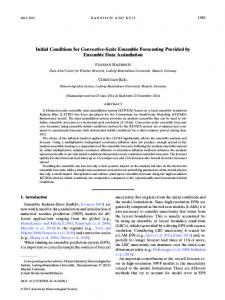
FIG. 1. Schematic of ensemble generation method. Sounding data are derived from the NCEP Meso Eta Model. The Memphis International Airport (MEM) is labeled, as is the Memphis WSR88D location (KNQA). Filled dots indicate grid points from which soundings are extracted; open circles show available soundings that are not used.

nized, deep convection. Nevertheless, the characteristics that qualitatively define a supercell storm within a cloud-scale simulation, for example, a positive correlation between vertical velocity w . 0 and vertical vorticity z . 0, are relatively insensitive to whether the microphysical processes are parameterized by the Kessler scheme or an explicit ice scheme (Klemp and Wilhelmson 1978; Weisman and Klemp 1982, 1984; Wicker and Wilhelmson 1995; Jewett et al. 1990; Johnson et al. 1993; Straka and Rasmussen 1998). For this work, the model is initialized with a horizontally homogeneous environment based on a single sounding, which implies that the storm initiates and evolves in an unchanging environment. This is clearly not what happens in the atmosphere where convective initiation and evolution are dependent upon mesoscale heterogeneity and forcing. This environmental restriction may limit the utility of the ensemble results. However, an ensemble of horizontally homogeneous models that sample a realistic variety of environmental conditions may yet display useful characteristics. Ensemble techniques generally use a set of initial conditions created by perturbing a base state. However, the best procedure for perturbing a base state is unclear when thermodynamic and kinematic sounding variability are considered over a relatively small region typical of where thunderstorms occur. As a consequence, initial conditions for this ensemble are, instead, generated using the variability inherent in time and space over a given region. That the variability in the initial conditions is not derived from a single base state (or control) is a fundamental difference between this method of generating initial conditions and the method used by SandicRancic et al. (1997).

Initial conditions are provided by soundings extracted from the NCEP Mesoscale Eta Model forecasts (Black 1994). The Meso Eta Model output is provided on the Advanced Weather Interactive Processing System (AWIPS) 212 grid. One sounding is used for each ensemble member. The output AWIPS 212 grid has a 40km horizontal grid spacing and a 25-hPa vertical grid spacing. Each ensemble member consists of a 2-h COMMAS cloud model run, initialized using a different forecast Meso Eta Model sounding. Because this work examines the potential for real-time use of mesoscale model output to initialize an ensemble of cloud models, any ‘‘contamination’’ of the initial soundings by convective parameterization schemes is ignored. This ensemble work is centered on two Integrated Terminal Weather System (Wolfson et al. 1997) testbed sites: Memphis, Tennessee, and Dallas–Fort Worth, Texas. Radar data from the associated WSR-88Ds (KNQA and KFWS, respectively) are used for verification. There are no observed soundings available from these sites, but they are convenient to use because MacKeen et al. (1999) provides a thorough analysis of convective storm lifetimes for the days examined. Thirteen soundings for initial conditions are extracted from alternate grid points on a 5 3 5 grid centered on the area of interest. The soundings come from the 0300 UTC Meso Eta Model runs that verify at 1800, 2100, and 0000 UTC. With 13 soundings at each of three forecast times, there are 39 sets of initial conditions for a 39-member COMMAS forecast ensemble (Fig. 1). All cases come from the summers of 1995 and 1996. Forecast fields are available at 3-h intervals from the Meso Eta Model, but only the 15-h forecast (valid at 1800 UTC), the 18-h forecast (valid at 2100 UTC), and the

APRIL 2002

ELMORE ET AL.

21-h forecast (valid at 0000 UTC) are used to create a daily ensemble. In one case (7 June 1996), the 21-h (0000 UTC), 24-h (0300 UTC), and 27-h (0600 UTC) forecasts are used. Using forecast soundings from three adjacent forecast times over a spatial domain implicitly recognizes temporal and spatial uncertainties in the forecast soundings. In principle, all soundings at all times are treated as equally likely at any location over a 9-h period, and the ensemble output is intended to be applicable across the entire region during the 9-h period. Hence, soundings originate from samples taken randomly from within a bounding volume defined in space and time. Any sounding from any spatial or temporal location is considered to be equally likely. This interpretation may not be strictly true and so may create a (probably slight) negative impact on the results. Initial conditions of the ensemble created by this method are called spatial–temporal atmospheric sampling and are fundamentally different from perturbations imposed upon a base state because no base state is defined. In the ideal, the ensemble of initial conditions represents equally likely initial states. In some instances, this ideal is violated intentionally. For example, dynamic conditioning methods, such as bred vectors or singular vectors (that is, processes that depend on the dynamical characteristics of the model), do not necessarily produce good samples of the forecast probability distribution. Instead, by design, these methods oversample the wings of the forecast probability distribution (Anderson 1996). Other times, the ideal is violated unintentionally. For the work presented here, soundings extracted from the mesoscale model output contain bias errors (Figs. 2a– d). When biases are present, the sampling function favors one wing of the true distribution. The biases are shown using data from the 0000 UTC Meso Eta Model analyses,1 which are available for 17 of the 18 cases (a 0000 UTC Meso Eta Model analysis is not available for 6 June 1995). For each forecast sounding valid at 0000 UTC, four parameters (potential temperature u, mixing ratio q, east–west wind component u, and north–wind component y ) are verified using the analyzed sounding derived from the next day’s 0000 UTC analyses. In terms of thermodynamics, these errors result in a boundary layer that is too warm and dry, a characteristic of the Meso Eta Model that existed during 1995 and 1996 (Marshall 1998). Wind errors are characterized by lowlevel southeasterly winds that are too strong and midlevel winds that are too northerly. There is unfortunately no good way to correct for these errors. Blindly correcting for the mean bias may not be appropriate for individual cases, because unrealistic vertical structures may result, and there is no way to know the errors for an individual case ahead of time. In addition, 95% confidence limits are used for forecasts of five bulk parameters that are known to be rel1 Analyses are used because there are no observed soundings at either Dallas–Fort Worth or Memphis.

367

evant to severe weather events. These bulk parameters are derived from the forecast soundings valid at 0000 UTC and are verified against analyzed soundings from the next day’s 0000 UTC analysis. These parameters are convective available potential energy (CAPE), lifted index (LI), storm relative helicity (SREH), bulk Richardson number (BRN), and the shear from the bulk Richardson number (BRN shear; Bluestein 1993; DaviesJones et al. 1990; Doswell 1985). This analysis helps to answer questions about how well salient sounding features are forecast, regardless of how well any individual sounding level is forecast. Consistent with the previous verification characteristics, a t test on forecast mean LI versus analyzed mean LI indicates that forecast LI is significantly more positive (stable) than the LI derived from the analysis. Results are similar for CAPE; the forecast CAPE is significantly too low in comparison with the CAPE derived from the analysis. These statistical results are expected primarily because the low-level mixing ratio forecast by the Meso Eta Model is significantly less than the verification mixing ratio. Because these statistical results are derived from several days pooled together, there are times when, for example, the warm bias is large enough to overcome the dry bias, which results in a forecast CAPE that is larger than the analysis CAPE. For SREH, the null hypothesis (that the forecast and observed distributions are the same) cannot be rejected at the 95% significance level. This result is at least partially an artifact of the many summer days used, which are typified by low-shear environments. Analyzed SREH exceeds forecast SREH primarily when forecast SREH is greater than 50 J kg 21 . Hence, on days with significant shear, the forecast SREH is significantly too low. Because SREH is sensitive to storm motion, which is poorly forecast, there is no clear evidence that this bias error in SREH creates an associated bias error in storm lifetimes. In a similar way, the forecast BRN and BRN shear values are significantly smaller than the corresponding analysis values. Results are similar for log(BRN shear). These results are consistent with the preceding discussion. Understanding average bias errors in the ensemble initial conditions is only one aspect of the verification problem. The ensemble model results also depend upon the range of initial conditions. Because this particular cloud model ensemble depends upon forecast soundings, it is important to know if the forecast variability is an accurate depiction of the analyzed variability. To address this question, the variability in the 0000 UTC forecasts is compared with the variability in the 0000 UTC analyses. A Kolmogorov–Smirnov (KS; Blum and Rosenblatt 1972) test is used to determine if the forecast and analyzed perturbation distributions are different at each sounding level at the 95% significance level. In all cases, perturbation values are defined as perturbations from the daily mean value; for example, a9 5 (a 2 a i ), for

368


VOLUME 41

FIG. 2. A 95% confidence interval for (a) uerr , (b) qerr , (c) uerr , and (d) y err error. The vertical dashed line is 0 error. When the confidence interval (shaded region) contains the 0 line, the error is insignificant at the 95% confidence level.

a as the mean value and a i as the value at a particular grid point. For perturbation u9, only one level in the boundary layer has different forecast and analysis perturbation distributions (Fig. 3a). Significantly different distributions also exist for a few layers above 600 hPa. Except near the surface, the distribution of forecast q9 is indistinguishable from the distribution of analyzed q9 for most of the troposphere (Fig. 3b). The KS results above 200 hPa have no meaning because mixing ratio is, for all practical purposes, 0 at these levels. The distributions of forecast and analyzed u9 and y 9 components are statistically indistinguishable at all levels (Figs. 3c, d). At two levels near the tropopause, the forecast and analysis y 9 distributions are different, but this result is

not significant because, at 95% significance levels, 1 out of 20 cases will exceed the 95% confidence limits. Crook (1996) shows that variations of only 61 K and 61 g kg 21 in the boundary layer can make the difference in whether a storm forms. The biases in the mean fields clearly exceed these limits. Given these verification results, why proceed with the ensemble cloud model exercise? If the goal is to model explicitly (or deterministically) particular thunderstorms at particular locations, then proceeding is pointless because this goal is not achievable. Yet, these statistical results reveal nothing about day-to-day forecast errors and variability or how they might affect the range and distribution of modeled storms. Hence, the goal to extract the maximum

APRIL 2002

ELMORE ET AL.

369

FIG. 3. KS test results for the forecast vs the analysis perturbation distributions valid at 0000 UTC for (a) u, (b) q, (c) u, and (d) y . The vertical dashed line indicates the 95% significance level (p 5 0.05). Values to the left of this line indicate parent distributions that are different.

amount of data concerning the range and distribution of thunderstorm lifetimes from the Meso Eta Model may still be attainable. Nonzero mean biases in the initial conditions do not necessarily preclude a successful ensemble model application. 3. Ensemble output and verification Because the cloud model is initiated with an unbalanced warm bubble, nonphysical transient responses will occur early in the model run and may have longterm effects (Lilly 1990; Brooks 1992). To ensure that any resulting storms have lifetimes beyond the eddy turnover time, output from the first 30 min is ignored. Storm lifetimes are then based upon data extracted after

this period. These data are available every 63 s and consist of the global maximum vertical velocity w and the reflectivity (dBZ e ). Because the cloud-model domain is large enough to contain more than one active storm, there are weaknesses in this approach that result in systematic model errors when more than one storm at a time is active. Two kinds of errors can occur, called type-A (Fig. 4) and type-B (Fig. 5) errors. Type-A errors occur when two storms are active simultaneously, but one is always weaker than the other. Type-A errors occur in about 10% of the cases in this work. Type-B errors occur when one storm follows another in a serial fashion, such that w remains above the threshold longer than either storm lasts. Type-B errors can lead to a significant overesti-

370


FIG. 4. An example of a type-A error, in which a strong, longlived cell obscures a weaker, shorter-lived cell.

mate of storm lifetime and are potentially more serious than type-A errors. Type-B errors fortunately, are rare, and none affect the storm lifetimes in the study dataset. A subset of the same data used in MacKeen et al. (1999) is used here for verification. Eighteen days with observed convection are used, and eight of these are characterized by some kind of severe weather report (hail, wind, or tornado). One day is characterized by a severe squall line, and the rest are characterized by isolated convection. To be included in the verification dataset, a storm must meet three criteria: 1) its lifetime must be at least two volume scans, which is 12 min for volume coverage pattern (VCP) 21 and 10 min for VCP 11; 2) the maximum reflectivity must be at least 40 dBZ e ; and 3) the storm track must be entirely contained within an annulus of 30–125 km from the radar. This range interval is chosen to reduce radar-sampling problems that can affect the Storm Cell Identification and Tracking (SCIT; Johnson et al. 1995) algorithm when storms are too close to or too far from the radar. For about 5% of the storms, SCIT fails to associate storms correctly in time and space. This error is ameliorated by manually verifying storm tracks and removing from the verification dataset storms that are clearly misassociated. Because the first 30 min of each cloud model run is discarded, the longest storm lifetime that can be modeled is 90 min. Observed storm lifetimes, however, have no such intrinsic limit. To alleviate this inconsistency, observed storms that last longer than 90 min are truncated to a maximum lifetime of 90 min. Data conversely are extracted from the model approximately every minute, so the minimum detectable storm lifetime is 1 min. Because such a short-lived storm cannot be observed, a modeled storm must last at least 6 min before it is counted. Where appropriate, this storm is assigned a minimum lifetime of two volume scans (12 min for cases verified with VCP-21 data and 10 min for data verified with VCP-11 data).

VOLUME 41

FIG. 5. Depiction of type-B error, in which two separate cells overlap temporally in such a way that they are counted as one and appear as an anomalously long-lived cell.

Over the 18 days used in this work, there are 1481 observed storms and 531 simulated storms. Observed and simulated storm lifetimes from each day are transformed into nonparametric probability density functions (pdfs) with a Gaussian kernel density estimator (Silverman 1986). For storm lifetimes, the true domain pdf lies on the interval [0, `] minutes, but, for practical application, the numerical domain is [0, 100] minutes. The domain extends to 100 min to avoid problems inherent in density estimators when the density is not 0 near the end of the domain. The end value of 100 min is an arbitrary choice and is dependent primarily upon the kernel bandwidth; yet, it works well for this analysis. Kernel density estimates may be thought of as smoothed histograms. However, in this case, the smoothing is applied on a statistical scale. The smoothing is based on a Gaussian kernel with a standard deviation (‘‘bandwidth’’) of 3 min, which is itself a pdf. Kernel density estimates result in nonparametric, discrete pdfs over finite intervals. Working directly with pdfs avoids many problems inherent with histograms (Silverman 1986). When the same kernel density estimator is applied to both forecast and observed lifetimes, statistical comparison between the pdfs is possible by the procedures described below. The Euclidean distance2 (formally called the L 2 norm) provides one way to compare discrete pdfs (Fig. 6). The difference between two pdfs is unfortunately not determined uniquely by Euclidean distance. However, if the Euclidean distance between two pdfs is 0, the pdfs are identical. Hence, the smaller the Euclidean distance value between two pdfs is, the more similar are the pdfs. Observed storm lifetime can be based only on ob2 Euclidean distance is one of a family of such norms. Euclidean distance is convenient because the norm exists within a Hilbert space, which has geometric properties similar to Euclidean space. The Ll norm between two vectors x and y is given by dx,y 5 { | x 2 y | l }1/l , l $ 1.

APRIL 2002

ELMORE ET AL.

FIG. 6. Graphical example of the Euclidean distance between two pdfs. The length of each vertical dotted line is the difference between the two discrete pdfs at each discrete point. The Euclidean distance results when each difference is squared and the square root is taken of the sum of all the squared differences.

371

served reflectivity, but both forecast w and reflectivity can be used to forecast storm lifetime. One parameter may work better than another, however. To address which parameter to use, forecast results for all days are pooled into a single dataset. The threshold for forecast lifetimes based on w is varied from 5 to 15 m s 21 in 1 m s 21 increments, and, in a like manner, the threshold for forecast lifetime based on reflectivity is varied from 30 to 60 dBZ e in 2-dB increments. Overall, 11 different thresholds for w and 16 different thresholds for reflectivity are investigated. Discrete pdfs are computed based on each threshold of each parameter and are compared with the discrete pdf of the observed lifetime for the superset of all observed storms. The Euclidean distance is computed between the forecast lifetime pdf and the observed lifetime pdf and is plotted as a function of the threshold. In the ideal, as the Euclidean distance between the forecast and verification pdf decreases, the forecast pdf becomes a better representation of the observations. A clear minimum in the Euclidean distance between the forecast pdf of storm lifetime based on w and the observed storm lifetime pdf occurs at 8 m s 21

FIG. 7. Euclidean distance between forecast and observed pdfs as a function of threshold for both w (in black) and reflectivity (in gray); 95% confidence limits are shown by capped, vertical bars. Results derived from any value whose confidence interval contains the dotted line are statistically indistinguishable from results derived from the 8 m s 21 threshold.

372


VOLUME 41

FIG. 9. The 95% confidence bounds for forecast (shaded) and observed (crosshatched) lifetime pdfs based on the 8 m s 21 w threshold. The probability assigned to storm lifetimes is not expected to be statistically different at the 95% significance level where the two pdf confidence intervals overlap. FIG. 8. Cell lifetime threshold based on 8 m s 21 and 56-dBZ e thresholds. A least squares linear regression fit yields a slope less than 1, which indicates that, given a lifetime based on 8 m s 21 , the expected lifetime based on 56 dBZ e is shorter. The solid line is a linear regression fit to the data; the dashed line shows a line of perfect agreement.

(Fig. 7). Even though a reflectivity threshold of 56 dBZ e is statistically equal to the 8 m s 21 w threshold, only one-half of the storms that reach the 8 m s 21 threshold also reach the 56-dBZ e threshold. As a consequence, using the 56-dBZ e threshold limits the sample size available for constructing the storm lifetime pdf. Therefore, an 8 m s 21 w threshold from the ensemble provides the better estimate of observed storm lifetime. Even though the pdfs are different, this difference could occur by chance due to sampling even if the data samples come from indistinguishable populations. The pooled permutation procedure (PPP) is one way to determine whether the sampled populations are distinct (Preisendorfer and Barnett 1983). The PPP test results shown here use 5000 permutations. Confidence limits for the forecast and observed pdf can also be generated using 1000 bootstrap resamples (Efron and Tibshirani 1993). The 2.5 and 97.5 percentiles at each discrete location of the estimated pdf provide an estimate of the 95% confidence envelope about the true storm lifetime pdf. Where the envelope is narrow, the pdf estimate is stable, and where the envelope is wide the pdf estimate is less certain. 4. Results a. General results Results for all days combined are presented first, followed by results from individual days. When compared on a storm-by-storm basis, storm lifetimes based on the

56-dBZ e threshold are generally shorter than storm lifetimes based on the 8 m s 21 threshold (Fig. 8). In particular, when the 8 m s 21 threshold yields a lifetime of 90 min, the 56-dBZ e threshold yields lifetimes between 0 and 90 min. Such a broad range indicates that, in some cases, a vertical velocity of 8 m s 21 is maintained for 90 min but the reflectivity never exceeds 56 dBZ e . The PPP test indicates the parent population of lifetimes based on w is indistinguishable from the parent population of observed lifetime for only 4 out of the 18 cases. Hence, the PPP test indicates that in four cases the hypothesis that the ensemble pdf is statistically consistent with (though not identical to) the pdf of observed storm lifetimes cannot be rejected. In nine cases, the forecast pdf captures the correct range of thunderstorm lifetimes, even if the pdf itself produces incorrect probabilities for particular storm lifetimes when compared with the observations. The other nine cases underestimate the range of storm lifetimes to varying degrees. The overall observed lifetime pdf is bimodal, with the higher peak around 12 min and a secondary peak near 90 min. The first peak is likely an artifact of the minimum storm lifetime requirement of 12 min. The second peak is an artifact that results from truncating storm lifetimes to no greater than 90 min. In comparison, the pdf based on a w threshold of 8 m s 21 also has a peak at 12 min and a broadened area at 23 min. A secondary peak, which is too large, exists at 90 min (Fig. 9). Overall, too few storms with lifetimes between 35 and 75 min are generated within the ensemble, resulting in probabilities that are too low for the occurrence of such storms. These pdfs provide insight into limits imposed by the particular cloud modeling approach used in the ensemble. This modeling approach cannot account for interactions between storms or storm interactions with the mesoscale environment, which might account for some

APRIL 2002

373

ELMORE ET AL.

FIG. 10. Dallas–Fort Worth ensemble region overlaid with 40-km L1 distances, which are shown by dotted lines. The L1 regions are centered on ensemble grid points. County boundaries are gray.

of the differences between observed and forecast pdfs. A homogeneous initial environment may partially explain the excessive number of long-lived storms created by the ensemble model, because a storm that starts in a favorable environment cannot propagate into a less favorable one, and vice versa. The warm, dry bias in the Meso Eta Model boundary layer means the forecast environment was typically less favorable to deep convection than was the real atmosphere. This characteristic is clearly seen in the resulting forecast pdfs of storm lifetime. In addition, cloud-scale models tend to evolve storms too quickly, especially when using the Kessler microphysical parameterization (L. Wicker 1999, personal communication). Taken together, these tendencies also help to explain the dearth of storms with medium lifetimes. Contingency table statistics may be used to determine whether the locations of modeled storms provide information about where storms are observed. To simplify the geometry, the L1 norm (also known as a ‘‘Manhattan’’ or ‘‘taxicab’’ distance) is used to define the verification region (Fig. 10). A 40-km L1 distance draws diamonds around each ensemble grid point. The vertices of each diamond are at 640 km on the x and y axes. A correct forecast occurs when the model produces deep

FIG. 11. ROC diagram for cloud ensemble performance. Each point (labeled) shows the storm lifetime threshold value used to build the diagram. The total area under the ROC curve yields a measure of the overall system performance.

convection at a particular grid point and a storm is observed by radar in the diamond defined by the L1 distance from that point. A ‘‘miss’’ is defined when a storm occurs in the diamond and no storm is modeled. A false alarm is defined when modeled convection occurs but none is observed in the diamond around the grid point. A correct null forecast is self-explanatory. Four basic statistics are computed from these data: probability of detection (POD), false-alarm ratio (FAR), critical success index (CSI), and true skill score (TSS; Flueck 1987). All are described in the appendix. Substantial variability exists from day to day, but overall TSS 5 0.064, which shows that the ensemble displays no skill in helping to anticipate where convection might occur within the region (Table 1), a result that could have been anticipated based on Crook (1996). Such poor skill results because, when merged with the forecast Meso Eta Model soundings, the COMMAS model tends to create deep convection at every grid point for at least one forecast sounding time. Too much

TABLE 1. A 2 3 2 convection location statistics table. The ‘‘all days combined’’ column shows how well the ensemble identifies where convection occurs for all 18 days, combined, based on a 40-km L1 distance from a grid point. The ‘‘days with limited convection’’ column shows statistics similar to those of the all days combined column, given that convection does not occur everywhere in the ensemble domain. The ‘‘w-based severe’’ column shows how well the ensemble identifies days for which severe weather reports will occur within the ensemble region. Parameter

All days combined

Days with limited convection

w-based severe

POD FAR CSI TSS

0.615 0.385 0.598 0.064

0.786 0.389 0.524 0.202

0.625 0 0.625 0.625

374


VOLUME 41

FIG. 12. The 95% confidence limits (shaded area) for the difference between perturbation (a) u, (b) q, (c) u, and (d) y parameters associated with short- and long-lived storms. Perturbations are calculated using daily mean values. The vertical dashed line is the 0 difference line, which, when contained in the shaded region, indicates no significant difference at the 95% confidence level.

deep convection also may be related to the warm-bubble initiation procedure. However, four days occur on which COMMAS does not produce deep convection at every grid point (‘‘limited convection’’ days). For these days, TSS increases to 0.202. This improvement suggests some skill in predicting where convection is likely on days with limited convection. Does the ensemble display any skill at identifying days when severe weather occurs? For standard 2 3 2 statistics, a hit is scored when a principal component analysis (Elmore and Richman 2001) indicates the ensemble generates long-lived storms (storms with at least 60-min lifetimes) and severe weather is reported anywhere within the 160 km 3 160 km ensemble region. A miss occurs when severe weather is reported but no

long-lived storms are generated, and a false alarm occurs when long-lived storms are generated but no severe weather is reported. Correct nulls are again self-evident. For these days, TSS 5 0.625 (Table 1). Although the results are encouraging, only eight days exhibit severe weather, so these results must be interpreted cautiously. This TSS value suggests that there may be some utility in using a long-lived mode from the ensemble as a severe weather indicator. The relative operating characteristics (ROC) diagram (Fig. 11) provides yet another way of interpreting the overall ensemble system performance (Mason 1982). In an ROC diagram, the probability of false detection (POFD, sometimes called the false-alarm rate) is plotted against POD for various thresholds. The precise process

APRIL 2002

ELMORE ET AL.

375

used to build the ROC diagram is described in the appendix. For this work, the thresholds are storm lifetimes of 20, 30, 40, 50, 60, 70, and 80 min. Perfect system performance is represented by an area of 1 under the curve, a purely random process is represented by an area of 0.5, and perfect inverse performance (when a forecast of ‘‘event occurs’’ always corresponds to ‘‘no event’’ and vice versa) is indicated by an area of 0. The overall area is greater than 0.5, but most of the contribution to the positive area occurs for the shorter lifetimes. This result mirrors the fact that the cloud model ensemble does not generate enough storms with lifetimes between 35 and 75 min. These results indicate some marginal skill but likely suffer from a dataset that is too small. b. Sounding parameters as discriminants between long-lived versus short-lived storms When a large number of cloud model runs are available, the differences between soundings that create longlived storms and those that create short-lived storms can be addressed. If reliable indicators of storm longevity are revealed, then the need to run a cloud model ensemble is obviated, because an approximate lifetime can be extracted directly by examining certain sounding characteristics that may have been missed in earlier analyses of the Meso Eta Model soundings (Stensrud et al. 1997). As in Stensrud et al., various bulk sounding characteristics are examined to determine whether the ensemble results could have been predicted by careful examination of the initial conditions. To ensure distinct demarcation between short- and long-lived storms, a maximum lifetime of 40 min is used to define shortlived storms and a minimum lifetime of 60 min is used to define long-lived storms. Some characteristic in the perturbations might possibly discriminate between long- and short-lived storms. Because the ensemble sometimes creates long- and short-lived storms based on data from the same day, an obvious approach examines differences in perturbation values of the raw sounding parameters u, q, u, and y . To facilitate this investigation, perturbation values u9, q9, u9, and y 9 are constructed for each day. For example, a t test on the quantity (q9long 2 q9short), where q9long is the mean perturbation q associated with all long-lived storms and q9short is the mean perturbation q for all shortlived storms, is used to determine whether the mean perturbations are significantly different from 0 at any level. When examined this way, perturbation soundings unfortunately provide no discrimination for lifetime at the 95% significance level (Fig. 12). Parameter spaces are often used to help to discriminate between supercell-type storms and nonsupercelltype storms. Under the assumption that long-lived storms are similar to supercell-type storms, these parameter spaces may provide some discrimination. One commonly derived parameter space is maximum CAPE

FIG. 13. Forecast lifetime plotted as a function of max CAPE and BRN. The best discrimination is provided when CAPE is greater than 2000 J kg 21 and BRN is less than 60.

versus BRN, an approach similar to that used in Weisman and Klemp (1982). If the combination of these two parameters can discriminate between long- and shortlived storms, distinct clusters of points for each type will appear. For long-lived storms, there is at least some success because long-lived storms tend to exist in the area where CAPE exceeds 500 J kg 21 and BRN is less than 60 (Fig. 13). When BRN is less than 1000, many short lived-storms are unfortunately mixed in with longlived storms, and, because a few long-lived storms exist for BRN between 60 and 100, this discrimination is deficient. The boundary between long- and short-lived storms becomes more diffuse when CAPE is less than 1000 J kg 21 but considerably more distinct when CAPE exceeds 2000 J kg 21 . As a consequence, limited discrimination is provided with the phase space defined by CAPE and BRN. Another, related, parameter space compares the maximum CAPE with the BRN shear. This combination unfortunately provides limited discrimination between short- and long-lived storms because both are mixed together throughout the parameter space such that there is no distinct cluster that contains primarily one or the other (Fig. 14a). When only those days that produce both long-lived and short-lived storms are used, excluding all days when either only long- or short-lived storms result, no significant improvement is noted. In fact, the mixing of long- and short-lived storms is even more apparent (Fig. 14b). Storm type can be categorized based on observed storms with SREH as a parameter (Brooks et al. 1993). In one scenario, CAPE is plotted against SREH along with lines of constant energy-helicity index (EHI 5 CAPE 3 SREH/(160 000); Davies 1993). EHI has been proposed as a discriminator between storms that produce strong tornadoes and those that produce violent tornadoes. Modeled long-lived storms primarily occupy the

376


VOLUME 41

FIG. 14. Same as Fig. 13, but plotting max CAPE vs BRN shear for (a) all days combined, and (b) only those days that produced both short-lived and long-lived cells.

region where EHI is greater than 1.0, but short-lived storms unfortunately tend to exist everywhere within this parameter space where EHI is less than 1.0 (Fig. 15a). Thus, this parameter space does only part of the job, because conditions that preclude long-lived storms are not identified. Another variant on this parameter space uses SREH scaled by the minimum storm-relative wind as one dimension and the maximum mixing ratio as the other dimension (Brooks et al. 1994). Based on observations, this parameter space is further divided into three zones. Storms in the zone-1 environment tend to be of the low-

precipitation (LP) supercell type, zone 2 tends to contain tornadic storms, and zone 3 tends to contain storms that create extreme wind events that are not associated with tornadoes (Fig. 15b). This parameter space may be useful for discriminating between various observed storm types, but there is clearly no discrimination between modeled short- and long-lived storms. Additional parameter spaces defined by perturbations from daily mean values are also examined. These additional parameter spaces are perturbation BRN versus perturbation CAPE, perturbation BRN shear versus perturbation CAPE, and perturbation BRN versus pertur-

FIG. 15. Parameter-space graphs using SREH as a dimension. (a) Maximum CAPE vs SREH: the horizontal dashed line is the 0 SREH reference line; the solid and dashed curves are EHI 5 1.0 and EHI 5 2.5, respectively. (b) SREH scaled by the minimum storm-relative wind vs the maximum mixing ratio. Zone 1 contains observed LP supercells, zone 2 contains observed storms with tornadic mesocyclones, and zone 3 contains observed storms associated with extreme wind gusts (after Brooks et al. 1994).

APRIL 2002

ELMORE ET AL.

FIG. 16. Same as in Fig. 9, but for 14 Jul 1995.

bation SREH. It is clear that such perturbation values have meaning only for those cases in which both longand short-lived storms coexist. None of these combinations offers any discrimination between long- and short-lived storms (not shown). There evidently is no reliable way to determine ahead of time how long a modeled thunderstorm is going to last, even when the parent environmental sounding (instead of a less-representative proximity sounding) is known to great precision. Observational errors in environmental soundings will lead to even greater uncertainties. As a consequence, it appears that a cloud model is needed to estimate the storm lifetime given a particular sounding. This implies that an ensemble of cloud models is the only reliable method available to extract the range and distribution of storm lifetimes from mesoscale model output. c. Specific cases The 14 July 1995 case from the Memphis area is an example of good agreement between the forecast lifetime pdf and the observed lifetime pdf (Fig. 16). The only region without overlap between the two pdfs is between 60 and 83 min, which means the ensemble did not produce any storms with lifetimes in this range. Also, the ensemble produced relatively few storms with lifetimes approaching 90 min. Thus, the 2.5-percentile limit for that region of the forecast pdf is 0. However, very few storms with lifetimes approaching 90 min were observed because the 2.5-percentile limit for the observed lifetime pdf is also nearly 0. The PPP test indicates that, for this case, populations of observed and forecast storm lifetimes are indistinguishable. Nonparametric tests unfortunately tend to be more prone to typeII errors than are parametric tests because fewer assumptions can be made about the underlying parent population. This example unfortunately shows no ability to discriminate where convection may be expected, because

377

deep convection results at every available sounding location (Fig. 17). The TSS is 0 for such cases. The ensemble model output contains long-lived (lifetime greater than 60 min) storms, and severe wind events are reported on this day. The 6–7 June 1996 case is one of two from the Dallas–Fort Worth area. This case is distinctive because the standard forecast times of 1800, 2100, and 0000 UTC are not used on this day. Rather, forecast soundings for 0000, 0300, and 0600 UTC are used in the ensemble because when the standard forecast times are used only two short-lived storms occur on the northernmost grid points. Yet, a significant severe weather outbreak occurred on this day after 0000 UTC, as a short wave and associated dryline and cold front swept though the area. Hence, the times for the ensemble initial conditions center upon the times of reported events. For this case, the ensemble does not generate enough storms to construct a representative forecast pdf of storm lifetime. A comparison between the pdfs that describe forecast and observed lifetimes is not meaningful because there are not enough storms produced by the ensemble for reliable pdf estimates. One indication that the sample size is too small is that the lower bound for the forecast pdf is everywhere 0 except around 90 min (not shown). Only 10 storms are produced within the ensemble, and, of these 10, 5 last 92 min. As a consequence, only six different lifetime estimates can be resampled, so the nature of the parent population from which the sample of forecast lifetimes is drawn cannot be characterized. Because the forecast lifetime pdf cannot be estimated well, it is no surprise that the PPP test shows significant differences between the observed and forecast parent distributions of storm lifetime. Despite these pdf results, this ensemble forecast has the exemplary quality that it captures the spatial distribution of convection well (Fig. 18). The ensemble generates long-lived storms where severe weather is reported, which means that the ensemble is useful for severe weather guidance in this case. The 2 3 2 statistics for this case are very good, with POD 5 0.750, FAR 5 0.400, CSI 5 0.500, and TSS 5 0.528. Forecasters could use output from this ensemble to maintain an especially careful watch on the region from the Dallas– Fort. Worth area northward. Another straightforward application of the ensemble data is to create conditional storm decay forecasts based on the current age of a particular observed storm (Fig. 19). These conditional pdfs are Bayesian in nature because the conditional storm lifetime, given by probability P(storm lifetime | storm has survived for t minutes), is computed using the forecast pdf after it is adjusted for the current storm age. The forecast pdf is adjusted for the age of a storm by truncating that part of the forecast pdf from t 5 0 to t 5 current storm age and rescaling the remainder of the forecast pdf to an area of 1. Thus, the probability that a storm will decay within a specified period of time beyond the current

378


VOLUME 41

FIG. 17. Observed storm locations near Memphis for 14 Jul 1995. Gray crosses show locations for all storms that last 30 min or less, and lighter crosses show the same for cells that last longer than 30 min. Gray dots represent locations that generate soundings that result in deep convection (defined as a cell that lasts longer than 6 min with w at least 8 m s 21 ) within the ensemble model. Lines show the 40-km L1 distance from each location. Skill scores are shown at the bottom of the figure. The W symbol shows the location of a severe wind report between the hours of 1630 UTC 14 and 0120 UTC 15 Jul 1995.

storm age can be calculated. Subtracting this storm decay probability from 1 yields the probability that the storm survives beyond a given age (Fig. 20). This information can be displayed easily as part of a storm track on a radar display (Fig. 21). Such a display provides NWS forecasters with guidance about the likelihood that a particular storm will affect a given community. Other characteristics derived from an ensemble can be encoded along the projected track, such as the probability of a mesocyclone, as defined by a positive correlation between vertical velocity and vertical vorticity. The projected storm tracks could be created with a 95% probability confidence interval using the pdf of storm motion for storms at various ages. Forecasts based on

pdfs have an elegant appeal because, once pdfs of a particular characteristic are constructed, creating probabilistic forecasts for that characteristic is easy. 5. Conclusions Various indices, parameters, and parameter spaces derived from forecast soundings are examined to determine whether any can provide reliable insight into the range or distribution of forecast storm lifetimes that can be expected on a given day. Though this examination is not exhaustive, none of the indices or parameters proved to be reliable discriminators between short-lived and long-lived storms. This result is not surprising because such parameters do not uniquely define a partic-

APRIL 2002

ELMORE ET AL.

379

FIG. 18. Same as Fig. 17, but for Dallas–Fort Worth for 6–7 Jun 1996. Black dots represent locations whose soundings do not generate deep convection. The H symbols show location of hail reports that meet or exceed severe criteria.

ular sounding. It consequently is unlikely that further refining the storm lifetimes into more categories such as short, medium, and long will prove useful. Therefore, the next logical approach is to use an ensemble of cloudscale models to forecast the distribution of storm lifetimes. Because only cases with convection are used, an analysis that examines how useful this ensemble might be for creating unconditional, probabilistic forecasts of convection is precluded. Because the ensemble tends to generate long-lived storms on days that experienced severe weather, storms with lifetimes longer than 60 min may be a useful indicator of severe weather. In a similar vein, if convection does not occur at all the locations from which initial soundings are drawn (limited convection), the ensemble results display some skill in identifying where thunderstorms will occur. However, only a handful of cases with either severe weather or limited

convection have been examined. These results are encouraging, but more cases must be analyzed to know if forecast storm lifetime is a useful proxy for severe weather occurrence and whether any skill exists in identifying where convection is likely to occur. Uncertainties in the forecast and observed pdfs of storm lifetime are estimated with bootstrap resampling. When the uncertainties implied by bootstrap sampling are considered, agreement between forecasts and observations is surprisingly good in light of the bias demonstrated in the ensemble of initial conditions. When considering the range of thunderstorm lifetimes, 50% of the forecast pdfs captured the correct range, and 50% underestimated the range by varying degrees. The PPP test indicates that in four cases the hypothesis that the ensemble pdf is statistically consistent with (though not identical to) the pdf of observed storm lifetimes cannot be rejected, although there is some evidence that the

380


FIG. 19. Conditional cell survival probability for KNQA, 8 Aug 1996. The vertical dashed line shows the current age of the thunderstorm. The pdf to the right of this line has been rescaled such that the area beneath the pdf is unity. Gray area represents the part of the pdf that no longer applies because the storm has already existed for 30 min. The hatched area yields the probability the storm has a lifetime between 30 and 35 min. The crosshatched area yields the probability that the cell has a lifetime between 35 and 40 min. The sum of the hatched and crosshatched areas yield the probability that the cell has a lifetime between 30 and 40 min.

PPP test may lack sufficient power to discriminate reliably between samples drawn from significantly different populations. When all the forecast and observed storm lifetimes are combined, the overall probability of storms with lifetimes between 35 and 75 min is too low and may be due to the modeled storms evolving too quickly (L. Wicker 1999, personal communication). Although these results are encouraging, this work is preliminary, and the results raise as many questions as they answer. For example, the Meso Eta Model no longer exists, having been incorporated into the current Eta Model. Various parameterizations within the Eta Model have been changed or modified. How these changes affect the cloud-scale ensemble model results is unknown. A broader question concerns which mesoscale model to use. One way to investigate this problem, and many other questions, is simultaneously to develop and to maintain an archive of radar data from various sites and an archive of output from operational forecast models. The archived operational model output may then be used to create initial conditions for cloud-scale ensembles. Once the ensembles are run, the output is verified against the archived radar data. Days chosen for the ensemble runs were dependent upon the available verification data. This restriction also determined the nature of days examined with the ensemble to those with relatively weakly sheared environments. Yet, most significant severe weather occurs in strongly sheared environments. How the ensemble performs in such cases has yet to be explored. Cloud-scale models also are sensitive to the geometry and strength of the warm bubble used to initiate con-

VOLUME 41

FIG. 20. The conditional survival probability for KNQA, 8 Aug 1996, computed from Fig. 19. The x axis shows the cell survival time beyond the current cell age. The y axis is the probability of survival beyond the current cell age. The horizontal dashed lines show probability thresholds of 50% and 25%.

vection (Lilly 1990; Brooks 1992), but the nature of this sensitivity is not understood well. Warm bubbles clearly have weaknesses when used to initiate convection, but they remain the most economical initialization scheme available. How the initiation procedure affects the ensemble results remains unknown. Cloud-scale model results are known to be sensitive to the parameterized precipitation physics (Jewett et al. 1990; Johnson et al. 1993; Straka and Rasmussen 1998). The cloud-scale model applied to this ensemble uses the Kessler scheme to parameterize precipitation physics. Ample evidence exists (L. Wicker 1999, personal communication; Johnson et al. 1993) that the Kessler scheme can lead to unrealistic storm evolution by significantly accelerating certain cloud-scale processes, which can cause unrealistically short lifetimes. If, instead, an appropriate ice microphysics package is used, more storms lasting between 35 and 75 min might occur, producing better overall forecasts of the pdfs of storm lifetime. A cloud-scale ensemble like the one described here is operationally practical. The available lead time depends on the mesoscale forecast lead time used to generate the initial conditions. For example, the entire ensemble will execute in 2.8 h on a 40-node Beowulf cluster consisting of 400-MHz Intel, Inc., Pentium-III processors and sufficient RAM to keep the cloud model grids memory-resident. Hence, if the same forecast times used in this paper are used operationally and the 0000 UTC operational model output used for the initial conditions is available by 0600 UTC, results for the ensemble would be available to forecasters by 0900 UTC. Such execution times yield roughly 7.5 h of lead time for the same forecast window examined here and are clearly operationally practical.

APRIL 2002

381

ELMORE ET AL.

FIG. 21. Conditional cell survival product for KNQA, 8 Aug 1996. The previously observed cell positions are shown in white. Projected cell positions are shown in color. With at least 50% probability, the cell will survive to some point along the red part of the projected track. With probability between 25% and 50%, the cell will survive to some point along the yellow part of the track. With probability less than 25%, the cell will survive to some point along the green part of the track. The depicted storm actually lasted another 42 min, for a total lifetime of 72 min.

Acknowledgments. The authors thank Dr. Louis J. Wicker of NSSL for generously providing his numerical cloud model for this study. Dr. Harold Brooks of NSSL provided insight into verification methods, and Dr. Michael B. Richman of the University of Oklahoma freely gave his advice concerning statistical approaches. Ms. Pamela MacKeen of NSSL has freely provided her time to help with using SCIT. Mr. Phillip Spencer of NSSL kindly provided modified versions of his Near-Storm Environment software, which was used to extract Meso Eta Model soundings from the AWIPS 212 grid. Mr. Geoff Manikin of NCEP graciously found the needed 0000 UTC Meso Eta Model analyses and made them available via FTP with facilities provided by the Environmental Modeling Center of NCEP. The authors also

thank the four reviewers who provided thoughtful comments and suggestions during the review process. Partial support for this research was provided through funds from the U.S. Weather Research Program of the National Atmospheric and Oceanic Administration. APPENDIX Description of Statistical Methods Many notations are used to describe 2 3 2 contingency tables. Here, a is the number of correct forecasts (hits), c is the number of missed detections (misses), b is the number of times convection is forecast and does not occur (false alarms), and d is the number of correct

382


VOLUME 41

POD 5

a , a1c

(A1)

Each day generates a set of 2 3 2 contingency tables, one for each lifetime threshold. To generate a grand table for each threshold, let A be the sum of all as over all days, B be the sum of all bs, and so on, at each threshold. From these grand tables, an ROC diagram for the ensemble system can be generated.

POFD 5

b , b1d

(A2)

REFERENCES

FAR 5

b , a1b

(A3)

nulls, which means no convection is forecast and none is observed (Table A1). Some statistics available from the 2 3 2 contingency table are given by

CSI 5

a , a1b1c

TSS 5

ad 2 bc . (a 1 c)(b 1 d )

and

(A4) (A5)

TSS possesses some appealing characteristics. Random forecasts, in which a random forecast is based on the same relative frequency as the observed event frequency, and constant forecasts, such as ‘‘no convection,’’ receive a 0 score. Also, the contributions of correct ‘‘no-event’’ and correct ‘‘yes’’ (hit) forecasts increase as the event is more or less likely, respectively. Hence, forecasts of rare events are not discouraged based solely on their low relative frequency. For constructing an ROC diagram, the entries in Table A1 have a different interpretation. For each storm on a given day, the ensemble provides P(lifetime $ x), the probability that the storm lasts at least x minutes. Hence, it is a simple matter to determine how many storms last longer than x and how many do not. In this case, a 1 b is the forecast number of storms that last longer than x (a yes forecast), and c 1 d is the forecast number of storms that do not last longer than x (a no forecast). As an example, let the lifetime threshold be 60 min and suppose that the ensemble P(x 5 60 min) 5 0.40. Further, suppose that 100 storms are observed. If the ensemble forecast is perfect, 40 storms will last 60 min or longer. However, suppose the observations show that only 30 storms last 60 min or longer. Hence, a 5 30, b 5 10, c 5 0, and d 5 60. Now consider the case when observations show that 50 out of the 100 storms last longer than 60 min. Here, a 5 40, b 5 0, c 5 10, and d 5 40. TABLE A1. A 2 3 2 contingency table, from which is computed FAR, POD, POFD, CSI, and TSS. The rows labeled ‘‘forecast’’ describe whether an event is forecast, and the columns labeled ‘‘observed’’ describe whether an event is observed. Observed Yes

No

Yes

a

b

No

c

d

Forecast

Anderson, J. L., 1996: A method for producing and evaluating probabilistic forecasts from ensemble model integrations. J. Climate, 9, 1518–1530. Battan, L. J., 1953: Duration of convective radar cloud units. Bull. Amer. Meteor. Soc., 34, 227–228. Black, T. L., 1994: The new NMC Mesoscale Eta Model: Description and forecast examples. Wea. Forecasting, 9, 265–278. Bluestein, H. B., 1993: Synoptic-Dynamic Meteorology in Midlatitudes. Vol. 2, Observations and Theory of Weather Systems, Oxford University Press, 594 pp. Blum, J. R., and J. I. Rosenblatt, 1972: Probability and Statistics. W. B. Saunders, 549 pp. Brooks, H. E., 1992: Operational implications of the sensitivity of modeled thunderstorms to thermal perturbations. Preprints, Fourth Workshop on Operational Meteorology, Whistler, BC, Canada, Atmos. Environ. Services/Canadian Meteor. Oceanogr. Soc., 398–407. ——, C. A. Doswell III, and R. A. Maddox, 1992: On the use of mesoscale and cloud-scale models in operational forecasting. Wea. Forecasting, 7, 120–132. ——, ——, and L. J. Wicker, 1993: STORMTIPE: A forecasting experiment using a three-dimensional cloud model. Wea. Forecasting, 8, 352–362. ——, ——, and J. Cooper, 1994: On the environments of tornadic and nontornadic mesocyclones. Wea. Forecasting, 9, 606–618. Browning, K. A., 1964: Airflow and precipitation trajectories within severe local storms which travel to the right of the winds. J. Atmos. Sci., 21, 634–639. Byers, H. R., and R. R. Braham, 1949: The Thunderstorm. U.S. Government Printing Office, 187 pp. Crook, N. A., 1996: Sensitivity of moist convection forced by boundary layer processes to low-level thermodynamic fields. Mon. Wea. Rev., 124, 1767–1785. Davies, J. M., 1993: Hourly helicity, instability, and EHI in forecasting supercell tornadoes. Preprints, 17th Conf. on Severe Local Storms, St. Louis, MO, Amer. Meteor. Soc., 107–111. Davies-Jones, R., D. Burgess, and M. Foster, 1990: Test of helicity as a tornado forecast parameter. Preprints, 16th Conf. on Severe Local Storms, Kananaskis Park, AB, Canada, Amer. Meteor. Soc., 588–592. Doswell, C. A., III, 1985: The operational meteorology of convective weather. Vol. 2: Storm scale analysis. NOAA Tech. Memo. ERL ESG-15, 240 pp. Efron, B., and R. J. Tibshirani, 1993: An Introduction to the Bootstrap. Chapman and Hall, 436 pp. Ehnrendorfer, M., 1997: Predicting the uncertainty of numerical weather forecasts: A review. Meteor. Z., 6, 147–183. Elmore, K. L., and M. B. Richman, 2001: Euclidean distance as a similarity metric for principal component analysis. Mon. Wea. Rev., 129, 540–549. Evans, J. E., 1997: Operational problem of convective weather in the national airspace system. Preprints, Convective Weather Forecasting Workshop, Long Beach, CA, Amer. Meteor. Soc. A1– A14. Flueck, J. A., 1987: A study of some measures of forecast verification. Preprints, 10th Conf. on Probability and Statistics in Atmospheric Sciences, Edmonton, AB, Canada Amer. Meteor. Soc., 69–73. Henry, S. G., 1993: Analysis of thunderstorm lifetime as a function

APRIL 2002

ELMORE ET AL.

of size and intensity. Preprints, 26th Conf. on Radar Meteorology, Norman, OK, Amer. Meteor. Soc., 138–140. Hou, D., E. Kalnay, and K. K. Droegemeier, 2001: Objective verification of the SAMEX ’98 ensemble forecasts. Mon. Wea. Rev., 129, 73–91. Houze, R. A., 1993: Cloud Dynamics. Academic Press, 573 pp. Jewett, B. F., R. B. Wilhelmson, J. M. Straka, and L. J. Wicker, 1990: Impact of ice parameterization on the low-level structure of modeled supercell thunderstorms. Preprints, 16th Conf. on Severe Local Storms. Kananaskis Park, AB, Canada, Amer. Meteor. Soc., 275–280. Johns, R., and J. A. Hart, 1993: Differentiating between types of severe thunderstorm outbreaks: A preliminary investigation. Preprints, 17th Conf. on Severe Local Storms, Saint Louis, MO, Amer. Meteor. Soc., 46–50. Johnson, D. E., P. K. Wang, and J. M. Straka, 1993: Numerical simulations of the 2 August 1981 CCOPE supercell storm with and without ice microphysics. J. Appl. Meteor., 32, 745–759. Johnson, J. T., P. L. MacKeen, A. Witt, E. D. Mitchell, G. J. Stumpf, M. D. Eilts, and K. W. Thomas, 1998: The storm cell identification and tracking algorithm: An enhanced WSR-88D algorithm. Wea. Forecasting, 13, 263–276. Kessler, E., 1969: On the Distribution and Continuity of Water Substance in Atmospheric Circulation. Meteor. Monogr., No. 32, Amer. Meteor. Soc., 83 pp. Klemp, J. B., and R. B. Wilhelmson, 1978: The simulation of threedimensional convective storm dynamics. J. Atmos. Sci., 35, 1070–1096. Kopp, F. J., and H. D. Orville, 1994: The use of a two-dimensional, time-dependent cloud model to predict convective and stratiform clouds and precipitation. Wea. Forecasting, 9, 62–77. Leith, C. E., 1974: Theoretical skill of Monte Carlo forecasts. Mon. Wea. Rev., 102, 409–418. Lilly, D. K., 1990: Numerical prediction of thunderstorms—has its time come? Quart. J. Roy. Meteor. Soc., 116, 779–798. Lorenz, E. N., 1963: Deterministic nonperiodic flow. J. Atmos. Sci., 20, 130–141. MacKeen, P. L., H. E. Brooks, and K. L. Elmore, 1999: Radar-reflectivity derived thunderstorm parameters applied to storm longevity forecasting. Wea. Forecasting, 14, 289–295. Marshall, C. H., 1998: Evaluation of the new land-surface and PBL parameterization schemes in the NCEP Mesoscale Eta Model using Oklahoma Mesonet observations. M.S. thesis, University of Oklahoma, 176 pp. Mason, I., 1982: A model for assessment of weather forecasts. Aust. Meteor. Mag., 30, 291–303. McNider, R. T., and F. J. Kopp, 1990: Specification of the scale and magnitude of thermals used to initiate convection in cloud models. J. Appl. Meteor., 29, 99–104.

383

Preisendorfer, R. W., and T. P. Barnett, 1983: Numerical model-reality intercomparison tests using small sample statistics. J. Atmos. Sci., 40, 1884–1896. Rogers, R. R., 1976: A Short Course in Cloud Physics. Pergamon, 227 pp. Schwartz, B. E., C. F. Chappell, W. E. Togstad, and X. Zhong, 1990: The Minneapolis flash flood: Meteorological analysis and operational response. Wea. Forecasting, 5, 3–21. Silverman, B. W., 1986: Density Estimation for Statistics and Data Analysis. Chapman and Hall, 175 pp. Sindic-Rancic, G., Z. Toth, and E. Kalnay, 1997: Storm scale ensemble experiments with the ARPS model: Preliminary results. Preprints, 12th Conf. on Numerical Weather Prediction, Phoenix, AZ, Amer. Meteor. Soc., 279–280. Stensrud, D. J., J. V. Cortinas Jr., and H. E. Brooks, 1997: Discriminating between tornadic and nontornadic thunderstorms using mesoscale model output. Wea. Forecasting, 12, 613–632. ——, J. W. Bao, and T. T. Warner, 2000: Using initial condition and model physics perturbations in short-range ensemble simulations of mesoscale convective systems. Mon. Wea. Rev., 128, 2077– 2107. Straka, J. M., and E. N. Rasmussen, 1998: Thirty years of cloud modeling: Does the emperor wear clothes? Preprints, 19th Conf. on Severe Local Storms, Minneapolis, MN, Amer. Meteor. Soc., 342–347. Weisman, M. L., and J. B. Klemp, 1982: The dependence of numerically simulated convective storms on vertical wind shear and buoyancy. Mon. Wea. Rev., 110, 504–520. ——, and ——, 1984: The structure and classification of numerically simulated convective storms in directionally varying wind shears. Mon. Wea. Rev., 112, 2479–2498. Wicker, L. J., and R. B. Wilhelmson, 1995: Simulation and analysis of tornado development and decay within a three-dimensional supercell thunderstorm. J. Atmos. Sci., 52, 2675–2703. ——, M. P. Kay, and M. P. Foster, 1997: STORMTIPE-95: Results from a convective storm forecast experiment. Wea. Forecasting, 12, 388–398. Wilson, J. W., 1966: Movement and predictability of radar echoes. Environmental Science Services Administration Tech. Memo. IERTM-NSSL-28, 30 pp. [Available from National Technical Information Service, Operations Division, Springfield, VA 22161.] ——, N. A. Crook, C. K. Mueller, J. Sun, and M. Dixon, 1998: Nowcasting thunderstorms: A status report. Bull. Amer. Meteor. Soc., 79, 2079–2099. Wolfson, M. M., C. K. Mueller, and M. D. Eilts, 1997: Convective weather forecasting for FAA applications. Preprints, Seventh Conf. on Aviation, Range, and Aerospace Meteorology, Long Beach, CA, Amer. Meteor. Soc., 238–243.