SHORT-RANGE ENSEMBLE FORECASTING Jean Nicolau Météo-France 42, Avenue G. Coriolis, 31057 TOULOUSE cedex 01, France Tel : +33 5 61 07 85 32, Fax: +33 5 61 07 84 53, E-mail :
[email protected]
1. Introduction Short range forecasts do not use any probabilistic information. Although such forecasts are more and more skilful, some events remain unpredictable. Météo-France wishes now to use probabilistic forecasts at short range in order to get an assessment on extreme events risks. At the time being, ensemble forecasting seems to be the more simple and efficient tool to achieve these goals. Ensemble prediction is already used for medium range forecasting (Molteni et al. 1994 ; Toth and Kalnay, 1997). However, methods used in such ensembles can not be directly applied for the short range forecasting (Brooks et alt., 1995). Research has already been performed in this area and a short range ensemble system is operational at NCEP (Tracton et al. 1998; Stensrud et al. 1999). We are presenting here the description of an experimental ensemble developped at Météo-France in the PEACE (Prévision d’Ensemble A Courte Echéance) project. This ensemble is devoted to detect rare severe events such as storms in the short range (24-48h). Emphasis is put on assessing skill of predicting strong mean sea level pressure gradient probabilities.
2. PEACE system and dataset Because of heavy computational cost, the ensemble is limited to 11 members (10 perturbed + 1 control). It is based on the global spectral ARPEGE model (Courtier et al., 1991). This model has a stretched grid that i.e. a low resolution over the southern Hemisphere (especially over New-Zeland) and a high resolution over the Northern Hemisphere (especially over France). In the PEACE system, it is used with a nominal spectral truncature of T199 and a stretching coefficient of 3.5 (which corresponds to an equivalent grid mesh of about 20 km over France).
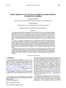
FIG. 1. Target area for the singular vector optimization (green) and verification area (red).
-2Initial perturbations used in the ensemble are generated by the singular vectors (SV) technic already used in the ECMWF EPS. One particular feature is the singular vectors optimization over a limited area including the Western Europe and the northern part of the Atlantic Ocean (see figure 1, green area). By this way, pertubations are believed to be efficient in the area of interest. Such targetting was already used for short-range to early-medium-range ensemble (Hersbach, 2000), to couple a global ensemble with a limited area model (e.g. Frogner, 2001). In our case no physics is used in the singular vectors computation (apart a simplified physics including diffusion). The total energy norm is used both at initial and final time with a T63 spectral troncature (the stretching is not used in SV computation). Time optimization is fixed to 12 hours. Five perturbations are built by combining the first 16 targetted singular vectors. Perturbed initial conditions are created by adding and substracting these perturbations to the unperturbed analysis. Then these 11 initial states are integrated up to 48h.This ensemble has been tested over a sample of 68 independent cases of observed or/and forecast storms between Dec. 1998 and April 2002.
3. Results Ensemble spread and mean error FIG. 2. shows the averaged spread (defined as the ensemble variance) for the geopotential height at 500 hPa as well as the Root Mean Square Error for the ensemble mean and the control forecast. Four main features appear : (1) EPS control obtains better results than the PEACE one ; (2) PEACE ensemble mean performs better than the PEACE control forecast (especially at 48h), (3) PEACE ensemble mean gets almost the same skill than EPS ensemble mean at 48h and (4) the spread for the PEACE ensemble is underestimated but its evolution follows quite well the ensemble mean error growth.
FIG. 2. 500hPA geopotential height spread and RMSE for different steps, averaged over the 68 cases sample for the EPS (green curves) and the PEACE ensmble (red curves)
Rank diagrams Rank histograms, also known as Talagrand diagrams (Talagrand et al., 1997), provide a useful measure of the reliability of an ensemble. FIG. 3. shows the rank diagrams for the temperature at 850 hPa (T850, top) the geopotential height at 500 (Z500, middle) and the Mean Sea Level Pressure (MSLP, bottom) at 48h. Concerning T850 it can be seen a U-shaped histogram which indicates an insufficient spread. This can be explained by the fact that no physics is used in the SV computation and no model perturbation is implemented. For Z500, the distribution is quite
-3flat indicating a good behavior for this parameter. The expected proportion of outliers for a perfect ensemble of 11 members is 2/(11+1) i.e. about 17%. For the Z500 rate is 21%. The MSLP rank histogram exhibits a strong bias toward the highest categories. This bias can be easily explained by the model tendency to be too much reactive and to produce deep lows. Tuning model diffusion parameters could reduce this bias.
FIG. 3. Rank diagrams over the whole sample at 48h for the temperature at 850hPa (left), geopotential heigh (right) and MSLP (bottom).
Probability scores One of the most important applications of the ensemble forecast is their use for generation of probabilistic forecasts. For a set of N forecasts of a binary event, the Brier score (BS, see Brier, 1950) is a measure of the skill of the probabilistic. The Brier Score was computed for the detection of the MSLP gradients for different thresholds; this parameter was chosen because strong gradients are the first mark of deep lows. In order to compare the accuracy of the forecast relative to the reference forecast (i.e. the EPS), the Brier Skill Score (BSS) was used. FIG. 4. gives the BSS score and its decomposition in resolution and reliability terms (see Atger, 1999 for more details). It can be seen that the PEACE ensemble performs better than the EPS especially for the high values of the threshold. The improvement of the BS reaches almost 40% at 6 hPa/100km.
-4-
FIG. 4. BSS (EPS used as reference) for the detection of MSLP gradients for different thresholds at 48h. BSS (red curve) is decomposed in reliability (green curve) and resolution (blue curve).
The improvement comes entirely from the resolution part. Both ensembles exhibit a similar reliability. In order to show the part of the model skill in the previous result, another BSS was computed, taking the control forecast as the reference. In this case, the forecast probability is equal to 1 if the event is forecast, 0 otherwise. FIG. 5. shows this BSS for the EPS and the PEACE ensemble for the same parameter (MSLP gradients for different thresholds) again at 48h. While the benefit from the ensemble is mainly important for the lower thresholds in the case of the EPS, the improvement for the PEACE ensemble remains between 30 and 40% even for the higher thresholds. Therefore it can be assessed that the good performance of the PEACE ensemble compared to the EPS comes mainly from the ensemble itself and not only from the model skill.
FIG. 5. BSS (Control forecast used as reference) for the detection of MSLP gradients for different thresholds at 48h.
One explanation to this particular feature could be the difference of each model resolution (nearly 80km for the EPS compared to 20km for the PEACE over the area of interest). The EPS lower resolution do not allow the system to produce strong gradients. One can observe the same feature by plotting hit and false alarm rates (HR and FAR) for the different probability value. For instance for the 30% probability class, the PEACE ensemble gets a HR great than 60% while its FAR remains lower than 50%, even for the higher thresholds (FIG. 6.). The HR of the EPS decreases to 0% for the higher thresholds while its FAR increases in the same time
-5reaching 100% for 9hPa/100km. The noisy curves for the EPS indicates that the event is nearly not forecast for the higher thresholds.
FIG. 6. Hit rate( dashed line) and false alarm rate (solid line) for the detection of MSLP gradients for different thresholds at 48h with 30% of probability.
4. Conclusions A prototype ensemble system has been developped for the detection of strong storms. It has been evaluated over a sample of different cases. It appears that although it presents a little lack of spread, it provides an acceptable and outperforms the EPS in MSLP gradients detection. This system is now running routinely once a day at 00UTC up to 48h. Different products will be developped and tested by operational forecasters during the next winter season. An example of probabilistic product is given in FIG. 7. The density of probability of low trajectories is plotted. In this case, deterministic trajectories from ECMWF model and the french model are inluded in plume of trajectories. Such a plot can give a very useful information to the forecaster on the most probable trajectory and its uncertainty.
FIG. 7. Example of probabilities of low trajectories - Model base : 20021012. Also plotted ARPEGE trajectory (blue) and ECMWF model trajectory (dashed green)
-6-
5. Future plans The development of this short range ensemble is in its first stage. Improvements will be necessary in different ways : • Inclusion of past errors in the initial state uncertainties sampling. This could be done by the implementation of a data assimilation ensemble. • Enhancement of model perturbations by tunning physical parametrizations and diffusion. • Use a limited area model (ALADIN) for the detection of heavy precipitation.
REFERENCES Atger, F. 1999 : The skill of Ensemble Prediction System. Monthly Weather Review: vol. 127, N°9, 1941-1953. Brier, G. W.,1950 : verification of forecasts expressed in terms of probability, Mon. Wea. Rev., 78, 1-3. Brooks, H. E., M.S. Tracton, D.J. Stensrud, G. DiMego, and Z. Toth, 1995: Short range ensemble forecasting: Report from a workshop, 25-27 July 1994, Bull.Amer.Meteor.Soc.,76,1617-1624. Courtier,P., Freydier,C., Geleyn,J.-F., Rabier, F., Rochas,M.1991. The ARPEGE project at Météo-France. In Workshop on numerical methods in atmospheric models. volume 2 pages 193-231, Reading, UK. ECMWF. Frogner, I.-L. and Iversen, T. 2001. High resolution limited area ensemble predictions based on low resolution targeted singular vectors. Submitted to Q. J. Roy. Meteor. Soc. Hersbach, H., R. Mureau, J. D. Opsteegh, J. Barkmeijer, 2000: A Short-Range to EarlyMedium-Range Ensemble Prediction System for the European Area. Monthly Weather Review: Vol. 128, No. 10, pp. 3501-3519. Molteni, F., R. Buizza, T.N. Palmer, T. Petroliagis, 1994: The ECMWF Ensemble Prediction System : methodology and validation, Technical Memorandum N° 202. Stensrud, D.J., H.E. Brooks, J.Du, M.S.Tracton, and E. Rogers, 1999: Using ensembles for short-range forecasting. Mon.Wea.Rev ., 127, 433-446. Toth, Z. and E. Kalnay, 1997: Ensemble forecasting at NCEP and the breeding method. Monthly Weather Review, 125, 3297-3319. Talagrand, O., B. Strauss and R. Vautard, 1997 : Evaluation of probabilistic prediction systems. Proc. Of the ECMWF Workshop on Predictability, Reading, United Kingdom, 1-25. Tracton, S., J. Du, Z. Toth, and H. Juang,1998:Short-range ensemble forecasting (SREF) at NCEP/EMC. Preprints, 12th Conf. on Numerical Weather Prediction. Phoenix, AZ, Amer. Meteor.Soc., 269-272.