Ensemble Extraction for Classification and Detection of Bird SpeciesI Eric P. Kasten∗,a,b , Philip K. McKinleyb , Stuart H. Gagea a
Remote Environmental Assessment Laboratory, Manly Miles Building, Room 101, Michigan State University, East Lansing, Michigan 48823 b Department of Computer Science and Engineering, Engineering Building, Michigan State University, East Lansing, Michigan 48824
Abstract Advances in technology have enabled new approaches for sensing the environment and collecting data about the world. Once collected, sensor readings can be assembled into data streams and transmitted over computer networks for storage and processing at observatories or to evoke an immediate response from an autonomic computer system. However, such automated collection of sensor data produces an immense quantity of data that is time consuming to organize, search and distill into meaningful information. In this paper, we explore the design and use of distributed pipelines for automated processing of sensor data streams. In particular, we focus on the detection and extraction of meaningful sequences, called ensembles, from acoustic data streamed from natural areas. Our goal is automated detection and classification of various species of birds. Key words: acoustics, data stream, ensemble, pattern recognition, remote sensing, time series analysis.
1. Introduction Advances in technology have enabled new approaches for sensing the environment and collecting data about the world; an important application domain is ecosystem monitoring (Porter et al., 2005; Szewczyk et al., 2004a; Martinez et al., 2004; Szewczyk et al., 2004b; Luo et al., 2007; Qi et al., 2008). Small, powerful sensors can collect data and extend our perception beyond that afforded by our natural biological senses. Moreover, wireless networks enable data to be acquired simultaneously from multiple geographically remote and diverse locations. Once collected, sensor readings can be assembled into data streams and transmitted over computer networks to observatories (Arzberger, 2004), which provide computing resources for the storage, analysis and dissemination of environmental and ecological data. Such information is important to improving our understanding of environmental and ecological processes. However, when data is collected continuously, automated processing facilitates the organization and searching of the resulting data repositories. Without timely processing, the sheer volume of the data might preclude the extraction of information of interest. Addressing these problems will likely become increasingly important as technology improves and more sensor platforms and sensor networks are deployed (The 2020 Science Group, 2005). I This work was supported in part by the U.S. Department of the Navy, Office of Naval Research under Grant No. N00014-01-1-0744, National Science Foundation grants EIA-0130724, ITR-0313142, and CCF 0523449, and a Quality Fund Concept grant from Michigan State University. ∗ Corresponding author Email addresses:
[email protected] (Eric P. Kasten),
[email protected] (Philip K. McKinley),
[email protected] (Stuart H. Gage) URL: http://www.real.msu.edu/∼kasten (Eric P. Kasten), http://www.cse.msu.edu/∼mckinley (Philip K. McKinley), http://www.real.msu.edu/∼gages (Stuart H. Gage)
Preprint submitted to Ecological Informatics
Acoustic signals have been used for many years to census vocal organisms. For example, the North American Breeding Bird Survey, one of the largest long-term, national-scale avian monitor programs, has been conducted for more than 30 years using human auditory and visual cues (Bystrak, 1981). The North American Amphibian Monitoring Program is based on identifying amphibian species primarily by listening for their calls (Weir and Mossman, 2005). Recent advances in sensor networks enable large-scale, automated collection of acoustic signals in natural areas (Estrin et al., 2003). The systematic and synchronous collection of acoustic samples at multiple locations, combined with measurements of ancillary data such as light, temperature, and humidity, can produce an enormous volume of ecologically relevant data. Transmuting this raw data into useful knowledge requires timely and effective processing and analysis. Acoustics as an ecological attribute has the potential to increase our understanding of ecosystem change due to human disturbance, as well as provide a measure of biological diversity and its subsequent change over time (Truax, 1984; Wrightson, 2000). The analysis of entire soundscapes may also produce valuable information on the dynamics of interactions between ecological systems in heterogeneous landscapes (Charles et al., 1999). Moreover, timely analysis and processing enables rapid delivery of important environmental information to those responsible for conservation and management of our natural resources, and can promote public involvement through public access to ready information about the environments in which we live. For instance, increased interest in renewable energy sources has driven the development of wind resource areas and the need to better understand the unintended impact of wind farms on wildlife. In turn, state and federal agencies have put forth guidelines for evaluating the potential effects that a wind farm might have on wildlife that include acoustic moniMarch 5, 2010
McKinley, 2007), a perceptual memory1 system that supports online, incremental learning. Results of our experiments are promising and suggest that extraction and analysis of ensembles from acoustic data may facilitate automated monitoring of natural environments. Moreover, the extraction of ensembles from acoustic clips reduced the amount of data to be processed by approximately 80%. The remainder of this paper is organized as follows. Section 2 describes background on the components of the ensemble extraction method. Section 3 describes in detail the approach for ensemble extraction, and Section 4 presents the results of our experiments using ensemble extraction for classification and detection of bird species. Section 5 presents related work. Finally, in Section 6, we conclude and describe future work.
toring (Michigan Department of Labor and Economic Growth, 2005; United States Fish and Wildlife Service, 2003; Anderson et al., 1999). This study addresses the automated classification and detection of bird species using acoustic data streams collected in natural environments. In this context, classification attempts to accurately recognize which species produced a particular vocalization, while detection indicates the likelihood that an acoustic clip contains a song voiced by a particular species. The project is a collaboration between computer scientists and ecologists at the Remote Environmental Assessment Laboratory (REAL) at Michigan State University. Acoustic data is collected from in field sensor stations located at the Kellogg Biological Research Station (KBS) in Michigan and other locations, some as far away Australia. Species classification and detection enables the automation of ecological surveys traditionally conducted by human observers in the field. Moreover, processing of data as it is collected enables annotation of sensor data with meta information that can facilitate later searching and analysis.
2. Background In this section, we first review methods used to represent and process acoustic data, including piecewise aggregate approximation (PAA) (Keogh et al., 2000; Yi and Faloutsos, 2000) and symbolic aggregate approximation (SAX) (Lin et al., 2003). Second, we describe a prototype system, Dynamic River, that we developed to enable automated, distributed processing of data streams. Finally, we review our earlier work with MESO (Kasten and McKinley, 2007), a perceptual memory system designed to support online pattern clustering and classification in data-intensive and time-sensitive applications. We use MESO for the classification and detection experiments described in Section 4. Time series processing. Figure 2 depicts two common methods for visualizing an acoustic clip. The top graph shows a plot of the signal’s oscillogram, and the bottom graph shows the same clip plotted as an acoustic spectrogram. A spectrogram depicts frequency on the vertical axis and time on the horizontal axis. Shading indicates the intensity of the signal at a particular frequency and time. Spectrograms are useful for visualizing acoustic signals in the frequency domain. Moreover, spectral representations can be used for automated classification and detection of acoustic events. In this study, for example, spectrogram segments are distilled into signatures that can be used to identify the bird species that produced a particular vocalization. To plot a spectrogram, the acoustic data is first divided into equal sized segments and then filtered using a Welch window to mitigate edge effects between segments. Then the discrete Fourier transform (Cooley and Tukey, 1965) is used to compute a frequency domain representation of each segment. Multiplying each value by its complex conjugate converts the complex representation used by the Fourier transform to a real representation of signal intensity. Finally, each segment is plotted to produce a spectrogram. Piecewise aggregate approximation (PAA) was introduced by Keogh et al. (Keogh et al., 2000), and independently by Yi
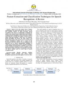
As shown in Figure 1, the acoustic sensor stations comprise a pole-mounted sensor unit and a solar panel coupled with a deep cycle battery for providing power over extended periods. Acoustic clips are collected by the sensor units and automatically transmitted to REAL over local and regional networks (e.g. over a local wireless network to the internet). When network technology is not available, manual collection may also be used. Currently, clips are approximately 30 seconds long and are collected every half hour. We anticipate increasing the collection rate as computing, storage and power resources permit. Sensor collection of acoustic data enables monitoring of natural environments despite visual occlusions, such as trees or buildings, or even darkness. Moreover, microphones can collect data from all directions simultaneously. However, acoustic data is rich and complex. For instance, bird vocalizations vary considerably even within a particular bird species. Young birds learn their songs with reference to adult vocalizations during sensitive periods (Thorpe, 1961; Tchernichovski et al., 2004). At maturity, the song of a specific bird will crystallize into a species-specific stereotypical form. However, even stereotypical songs vary between individual birds of the same species (Catchpole and Slater, 1995). Moreover, many vocalizations are not stereotypical but are instead plastic and may change with seasons, while some species can learn new songs throughout their lives (Brenowitz et al., 1997). Variation of song within a species and the occurrence of other sounds in natural settings, such as the sound of wind or that produced by human activity, are significant obstacles to automated detection and classification of birds. Extraction of candidate bird vocalizations from acoustic streams facilitates accurate recognition of a species. The main contribution of this paper is to introduce a process that enables detection and extraction of meaningful sequences, called ensembles, from acoustic data streams. Here we investigate the utility of this method to support automated detection and classification of bird species using MESO (Kasten and
1 Perceptual memory is a type of long-term memory for remembering external stimulus patterns (Fuster, 1995).
2
0
KHz 5.5
11 −1
Amplitude 0
1
Figure 1: Example sensor platform deployments. Deployment locations: (a) Michigan State Univeristy Lakes site, East Lansing, MI; (b) Pond Laboratory at the Kellogg Biological Station, Hickory Corners, MI; (c) Frog and toad Survey project wetland site, DeWitt, MI; and (d) Crystal Bog buoy deployment, Trout Lake, Wisconsin.
0
20 Seconds
10
30
38
Figure 2: Visualization methods. Top, an oscillogram (normalized) of an acoustic signal. Bottom, a spectrogram of the same acoustic signal.
and Faloutsos (Yi and Faloutsos, 2000), as a means to reduce the dimensionality of time series. For completeness a brief
overview of PAA is presented here; full details can be found in (Keogh et al., 2000; Yi and Faloutsos, 2000). As shown in 3
Figure 3, an original time series sequence, Q, of length n is converted to PAA representation, Q. First, Q is Z-normalized (Li and Porter, 1988) as follows: ∀i qi = (qi − µ)/σ, where µ is the vector mean of the original signal, σ is the corresponding standard deviation and qi is the ith element of Q. Second, Q is segmented into w ≤ n equal sized subsequences, and the mean of each subsequence computed. Q comprises the mean values for all subsequences of Q. Thus, Q is reduced to a sequence Q with length w. Each ith horizontal segment of the plot shown in Figure 3(b) represents a single element, qi , of Q. Thus, the complete PAA algorithm first Z-normalizes Q and then computes the segment means to construct Q, as depicted in Figure 3(b). Z-normalization and conversion to PAA representation affords two benefits that facilitate detection and classification. First, detection and classification using acoustics in natural environments is often impeded by variance in signal strength due to distance from the sensor station or differences between individual vocalizations. Z-normalization converts two signals that vary only in magnitude to two identical signals, enabling comparison of signals of different strength. Second, conversion to PAA representation helps smooth the original signal to facilitate comparison of vocalizations. Specifically, during classification or detection, signals are typically represented as vectors of values, called patterns. For acoustics, many pattern values may represent noise or sounds other than those voiced by a bird. These values do not contribute usefully when using distance metrics, such as Euclidean distance, for pattern comparison. PAA smoothes intra-signal variation and reduces pattern dimensionality, while Z-normalization helps equalize similar acoustic patterns that differ in signal strength. Figure 4 depicts a spectrogram for an acoustic signal before and after conversion to PAA representation. The spectrogram shown in Figure 4(b) was constructed by applying PAA to the frequency data comprising each column of the original spectrogram shown in Figure 4(a). Despite smoothing and reduction using PAA, these spectrograms are similar in appearance, demonstrating the potential utility of using PAA representation. For comparing patterns that have not been reduced using PAA, Euclidean distance can p be used. Euclidean distance is Pn 2 defined as: DEuclidean (Q, P) ≡ i=1 (qi − pi ) , where Q and P are two patterns of length n. Computing the distance between two patterns reduced using PAA is similar to computing Euclideanp distance. PAA distance is defined as: DPAA (Q, P) ≡ √ Pw 2 n/w i=1 (qi − pi ) , where Q and P are two patterns reduced using PAA. The terms n and w are the lengths of the original patterns and those after PAA reduction, respectively. PAA distance has been shown to be a tight lower bound on Euclidean distance (Keogh et al., 2000), providing a close estimate of Euclidean distance between the original two patterns despite PAA dimensionality reduction. Extending the benefits of PAA is a representation introduced by Lin et al. (Lin et al., 2003) called Symbolic Aggregate approXimation (SAX). The purpose of SAX is to enable accurate comparison of time series using a symbolic representation. As shown in Figure 5(a), SAX converts a sequence from PAA representation to symbolic representation, where each symbol (we use integers as symbols, others have used alphabetic charac-
ters (Lin et al., 2003)) appears with equal probability based on the assumption that the distribution of time series subsequences is Gaussian (Lin et al., 2003). Thus, each PAA segment is assigned a symbol by dividing the Gaussian probability distribution into α equally probable regions, where α is the alphabet size (α = 5 in Figure 5(a)). Each PAA segment falls within a specific Gaussian region and is assigned the corresponding symbol. Kumar et al. (Kumar et al., 2005) proposed time series bitmaps for visualization and anomaly detection in time series. SAX bitmaps are constructed by counting occurrences of symbolic subsequences of length n (e.g., 1, 2 or 3 symbols ). Each bitmap can be represented using an n-dimensional matrix, where each cell represents a specific subsequence. An example is shown in Figure 5(b); using subsequences of length n = 2, matrix cell (1, 1) contains the count and frequency with which the subsequence 1, 1 occurs. Frequencies are computed by dividing the subsequence count by the total number of subsequences. An anomaly score can be computed by comparing two bitmap matrices using Euclidean distance. The matrices are constructed using two concatenated sliding windows. For each anomaly score computed, both windows are moved forward along the time series one time step and the corresponding matrices computed. The distance between the matrices is computed and reported as an anomaly score. Greater distances indicate significant change in the time series. As further discussed in Section 3, we use SAX bitmap matrices to compute an anomaly score for acoustic signals, enabling the extraction of bird vocalizations and other acoustic events. Dynamic River. We have developed a prototype system, Dynamic River (Kasten et al., 2007), that enables the construction of a distributed stream processing pipeline. A Dynamic River pipeline is defined as a sequential set of operations composed between a data source and it’s final sink (destination). Network operators enable record processing to be distributed across the processor and memory resources of many hosts. Pipeline segments are created by composing sequences of operators, such as PAA and SAX, that produce a partial result important to the overall pipeline application. As depicted in Figure 6, segments can receive and emit records using the streamin and streamout operators, respectively, enabling instantiation of segments and the construction of a pipeline across networked hosts. Moreover, pipelines can be recomposed dynamically by moving segments among hosts. Preserving the integrity of data streams in the presence of a dynamic environment is a challenging problem. Dynamic River records can be grouped using record subtype, scope and scope type header fields. We define a data stream scope as a sequence of records that share some contextual meaning, such as having been produced from the same acoustic clip. Within the data stream, each scope begins with an OpenScope record and ends with a CloseScope record. Optionally, CloseScope records can be replaced with BadCloseScope records to enable scope closure while indicating that the scope has not reached its intended point of closure. For instance, if an upstream segment terminates unexpectedly and leaves one or more scopes open, the streamin 4
4
4
0
0
−4 0
1.5
−4 0
3
(a) original signal.
1.5
3
(b) Z-normalized signal with PAA
0
0
KHz
KHz
11
11
Figure 3: Example signal and results of Z-normalization and subsequent PAA processing.
0
Seconds
0
19
(a) original spectrogram.
Seconds
19
(b) PAA spectrogram
Figure 4: (a) Original spectrogram. (b) Spectrogram after processing with PAA (stretched vertically for clarity).
operator will generate BadCloseScope records to close all open scopes, Scopes can be nested. The scope field indicates the current scope nesting depth, larger values indicate greater nesting while scope depth 0 indicates the outermost scope. The scope type field enables the specification of an application specific scope type. For instance, a scope can be identified as comprising an acoustic clip or an ensemble. Optionally, OpenScope records may contain context information, such as the sampling rate of an acoustic clip. Scoping can also be used to support graceful shutdown and fault tolerance in streaming applications. MESO. For classification and detection experiments we use MESO2 (Kasten and McKinley, 2007), a perceptual memory system designed to support online, incremental learning and decision making in autonomic computing systems. MESO is based on the well-known leader-follower algorithm (Hartigan, 1975), an online, incremental technique for clustering a data set. A novel feature of MESO is its use of small agglomerative clusters, called sensitivity spheres, that aggregate similar training patterns. Sensitivity spheres are partitioned into sets during the construction of a memory-efficient hierarchical data structure. This structure enables the implementation of a contentaddressable perceptual memory system: instead of indexing by
an integer value, the memory system is presented with a pattern similar to the one to retrieve from storage. MESO can be used strictly as a pattern classifier (Duda et al., 2001) if a categorization is known during training. In this case, each pattern is labeled, assigning each pattern to a specific real-world category, such as a particular bird species. As shown in Figure 7(a), two basic functions comprise the operation of MESO: training and testing. During training, patterns are stored in perceptual memory, enabling the construction of an internal model of the training data. Each training sample is a pair (xi , yi ), where xi is a vector of continuous, binary or nominal values, and yi is an application-specific data structure containing meta-information associated with each pattern. The size of the sensitivity spheres is determined by a δ value that specifies the sphere radius in terms of distance (e.g. Euclidean distance) from the sphere’s center. Sensitivity sphere size is calculated incrementally, growing the δ during training. Figure 7(b) shows an example of sensitivity spheres for a 2D data set comprising three clusters. A sphere’s center is calculated as the mean of all patterns that have been added to that sphere. The δ is a ceiling value for determining if a training pattern should be added to a sphere, or if creation of a new sphere is required. Once MESO has been trained, the system can be queried using a pattern without meta-information. MESO tests the new pattern and returns either the meta-information associated with the most similar training pattern or a sensitivity sphere contain-
2 The term MESO refers to the tree algorithm used by the system (MultiElement Self-Organizing tree)
5
2
2 3 2 4 3 3 3 4 1 5 3 1 2 4 4 3 4 3
1.5 5
0
0
0
0
1
0
0
0
4
0 1 0.0
0
0.5
0.0
0.0
0.0
0.0
0.0
0.125
0.0
0.0
0.0
0
1
1
0
0
0
0
1
3
0.0
0.0
0.0
0.0
0.0
0.0
0.125
0
0
2 0
0.0
2
3
0
1
0
1
0
0
1
0
1
1 4 0.125
1
−0.5 −1 −1.5
0.0
0 SAX = 2
0.5
1
1.5
2
2.5
3
2
1
0.125 0.25 0.125
0.0
0.125
0.0
0.0
0.125
0.0
0
1
0
0
0
0
2
1
0
0.0
0.125
0.0
0.0
0.0
0.0
0
0
0
0
0
0
0.0
0.0
0.0
0.0
0.0
0.0
0.0
1
2
5 0
−2
0.125 0.125
3 2 4 3 3 3 4 1 5 3 1 2 4 4 3 4 3
(a) Conversion to SAX.
0.25 0.125
0.0
0
0
0.125 0.0
0.0
1
3 3 4 5 1 2 anomaly score = 0.433013
4
1 2 3 4 5
5
(b) Computing an anomaly score.
StreamIn
operator
stdout
stdin
RecordReader
RecordWriter
stdout stdin
Operator
socket
RecordReader
Loop: until [stdin.EOF = true]
RecordWriter
Loop: until [stdin.EOF = true]
RecordReader
Loop: until [socket.EOF = true]
RecordWriter
Figure 5: (a) Conversion of the example PAA processed signal to SAX (adapted from (Lin et al., 2003)), and (b) Using SAX bitmaps to compute an anomaly score for a signal (see (Kumar et al., 2005) for more information). Number of subsequences occurrences shown over frequency.
socket
StreamOut
Figure 6: Basic internal structure of basic stream operators and the streamin and streamout network operators.
ing a set of similar training patterns and their meta-information. When evaluated on standard data sets, MESO accuracy compares very favorably with other classifiers, while requiring less training and testing time in most cases (Kasten and McKinley, 2007).
Figure 8 depicts a typical approach to data acquisition and analysis using a Dynamic River pipeline that targets ecosystem monitoring using acoustics, and Table 1 provides a conscise description of the pipeline operators. First, audio clips are acquired by a sensor platform and transmitted to a readout operator that writes the clips to record for storage. Although additional record processing is possible prior to storage, it is often desirable to retain a copy of the raw data for later study. During analysis, a data feed is invoked to read clips from storage and write them to wav2rec to encapsulate acoustic data (WAV format in this case) in pipeline records. The remaining operators comprise the process for extracting ensembles and processing them for classification or detection using MESO, as follows.
3. Ensemble Extraction and Processing A sensor data stream is a time series comprising continuous or periodic sensor readings. Typically, readings taken from a specific sensor can be identified, and each reading appears in the time series in the order acquired. Online clustering or detection of “interesting” sequences benefits from time-efficient, distributed processing that extracts finite candidate sequences from the original time series. Our goal is to extract potentially recurring sequences that can be used for data mining tasks such as classification or detection. As noted earlier, we define ensembles as time series sequences that recur, though perhaps rarely. This definition is similar to other time series terms. For instance, a motif (Yi et al., 1998; Chiu et al., 2003; Lin et al., 2002; Tandon et al., 2004) is defined as a sequence that occurs frequently, and a discord (Keogh et al., 2005) is defined as the sequence that is least similar to all other sequences. A limitation for finding a discord in a time series is that the time series must be finite. Our use of ensembles addresses this limitation by using a finite window for computing an anomaly score and thereby detecting a distinct change in time series behavior. An anomaly score greater than a specified threshold is considered as indicating the start of an ensemble that continues until the anomaly score falls below the threshold.
The pipeline segment, saxanomaly→trigger→cutter, transforms records comprising acoustic data into ensembles. The incoming record stream is scoped, with each clip delimited by an OpenScope/CloseScope pair. The outgoing record stream comprises ensembles that are also delimited by an OpenScope/CloseScope pair. The clip and ensemble scopes are typed, using the scope type record header field, as scope clip or scope ensemble respectively. The moving average of the SAX anomaly score, as described in Section 2, is output by saxanomaly in addition to the original acoustic data. Parameters such as the SAX anomaly window size, SAX alphabet size and a moving average window size, can be set to meet the needs of a particular application or data set. The SAX anomaly window size specifies the number of samples to use for constructing each concatenated window used for computing the SAX anomaly score, for a given SAX alphabet. The moving average window size specifies the number of anomaly scores to use for computing a mean anomaly score that 6
20 Train
Test
Meta
15
Meta
Meta Meta Meta
10
Meta
5
0
MESO
0
(a) high-level view of MESO
5
10
15
20
(b) sensitivity spheres
Figure 7: MESO operation and sensitivity spheres (Kasten and McKinley, 2007). Depicted in (a) is the training and testing of MESO using patterns and associated meta-information. Sensitivity spheres for three 2D-Gaussian clusters are shown in (b). Circles represent the boundaries of the spheres as determined by the current δ. Each sphere contains one or more training patterns, and each training pattern is labeled as belonging to one of three categories (diamond, square, or triangle).
readout
1 0 0 1 0 1 0 1 0 1 0 01 1 0 1 0 1 0 1 0 1 0 1 0 1 0 1 0 1 0 01 1 0 1 0 1 0 1 0 1 0 1 0 1 0 1 0 1 0 01 1 0 1 0 1 0 01 1 0 1 Storage
record
Access Point
wav2rec
feed
Clips sax− anomaly
trigger
dft
float2cplx
cplxconj
cutout
cutter
Welsh window
paa
MESO
Ensembles
reslice
record2− vect
Processed Ensembles
Figure 8: Block diagram of pipeline operators for converting acoustic clips into ensembles for detection of bird species.
is output by saxanomaly as input to the cutter operator. Based on the mean anomaly score, the cutter operator extracts windows of anomalous behavior from the data stream. In our experiments with environmental acoustics, we set the moving average window to 2,250 samples (approximately 0.1 seconds), the SAX anomaly window to 100 samples and the SAX alphabet size to 8. Figure 9 depicts the anomaly score computed the by saxanomaly operator (top) for the signal depicted in Figure 2, the corresponding trigger signal output by the trigger operator (center) and the corresponding ensembles extracted from the original acoustic signal by the cutter operator (bottom). The trigger operator transforms the anomaly score output by saxanomaly into a trigger signal that has the discrete values of either 0 or 1. The trigger operator is adaptive in that it incrementally computes an estimate of the mean anomaly score, µ0 , for values when the trigger value is 0.
Trigger emits a value of 1 when the anomaly score is more than 5 standard deviations from µ0 and a 0 otherwise. The number of standard deviations is application specific. The cutter operator reads both the records containing the original acoustic signal and the records emitted by trigger. When the trigger signal transitions from 0 to 1, cutter emits an OpenScope record, designating the start of an ensemble, and begins composing an ensemble. Each ensemble comprises values from the original acoustic signal corresponding to trigger values of 1. When the trigger value transitions from 1 to 0, cutter emits a CloseScope record, and resumes consuming acoustic values until the trigger value again transitions to 1. The record stream, as emitted from cutter, comprises clips that contain one or more ensembles. The pipeline segment, reslice→welchwindow→ float2cplx→dft→cplxconj, transforms the amplitude data of each ensemble into a frequency domain (power spec7
Trigger Value Anomlay Score 0.5 1 2 0.4 0.5 1 0 Amplitude 0 −1 0
20 Seconds
10
30
38
Figure 9: Anomaly score, trigger signal and ensembles extracted from the acoustic signal shown in Figure 2.
4. Assessment
trum) representation in a way similar to that used to produce a spectrogram. First, for each pair of ensemble records, the reslice operator constructs a new record comprising the last half of the first original record and the second half of the second record. This new record is then inserted into the record stream between the two original records. Reslicing ensemble records is a method similar to that used by Welch’s method (Welch, 1967) for minimizing variance when computing power spectral density (PSD) using finite length periodograms.
Listed in Table 2 are the four-letter species codes and the common names for the 10 bird species whose vocalizations we used in our experiments. Also listed are the number of individual patterns and ensembles extracted from the recorded vocalizations and included in our experimental data sets. For testing classification accuracy, we used four data sets produced from a set of audio clips, and each extracted ensemble contains the vocalization from one of the 10 bird species. Although each ensemble contains the vocalization for only a single species, the clips typically contain other sounds such as those produced by wind and human activity. Ensemble data sets. Two ensemble data sets, comprising 473 ensembles, were produced using the method described in Section 3. The data sets differ in that one was processed with PAA while the other was not. The ensembles produced by the cutter operator were then fed to the dft (discrete Fourier transform) operator for further processing (refer to Figure 8). Each ensemble comprises one or more patterns. Each pattern was constructed by merging 3 frequency domain records. A single pattern represents 0.125 seconds of acoustic data in the range ≈[1.2kHz,9.6kHz] and comprises either 1,050 features or, when processed with PAA, 105 features. A voting approach is used for classifying each ensemble. Specifically, each pattern belonging to a given ensemble is tested once and represents a “vote” for the species indicated by the test. The species with the most votes is returned as the recognized species. Pattern data sets. Each of the two pattern data sets comprises 3,673 patterns extracted from the 473 ensembles in the ensemble data sets. Like the ensemble data sets, each pattern has either 1,050 or 105 features and represents 0.125 seconds of acoustic data. Ensemble grouping is not retained and, as such, recognition is based on testing with a single pattern.
The remainder of the pipeline segment, starting with welchwindow, computes a floating point representation of each ensemble’s spectrogram, where each ensemble comprises one or more records of spectral data. Next, each record of each ensemble is passed to the cutout operator. The cutout operator selects specific frequency ranges from each record and emits records comprising only these ranges. Data outside of the selected range is discarded. For our classification experiments, the frequency range ≈[1.2kHz,9.6kHz] was cutout. Frequencies above and below this range typically have little data useful for classification or detection of bird species. Moreover, data below this range typically comprises low frequency noise, including the sound of wind and sounds produced by human activity. For our detection experiments, discussed in Section 4, the cutout operator with smaller frequency ranges was used to further reduce the frequency range for better detection of specific species. The optional paa operator reduces each record to a PAA representation as discussed in Section 2. For our experiments, we used records containing 1,050 frequency power values to construct training and testing patterns. Each pattern comprised either the entire 1,050 frequency power values, or was reduced by a factor of 10 using PAA. The effectiveness of using PAA representation for smoothing acoustic spectral data is demonstrated in Section 4. Finally, the rec2vect operator converts pipeline records to vectors of floating point values (patterns), suitable for use in our classification and detection experiments with MESO.
4.1. Species Classification Experimental method. We tested classification accuracy using cross-validation experiments as described by Murthy et 8
Table 1: Description of Dynamic River data operators.
Table 2: Bird species codes, names and the number of patterns (Pat.) and ensembles (Ens.) used in the experiments discussed in Section 4.
Operator cplxconj
Description Convert an input record of complex values to a record of comprising the complex conjugate values of the input record. cutout Convert an input record of floating point values by selecting a specific range of values and discarding the remainder. cutter Expects both a data record and a trigger record as input and emits records comprising input data record segments that correspond to when the input trigger record values are 1 (see trigger below). dft Convert an input record of complex values by computing the discrete Fourier transform. float2cplx Convert an input record of floating point values to a complex number representation. Specifically, the real part of the imaginary number contains the original floating point value and the imaginary part is set to 0. paa Convert an input record of floating point values using piecewise aggregate approximation (PAA). rec2vect Convert an input record to a vector of floating point values. reslice Convert each pair of input records to 3 output records by inserting a record comprising the last half of the first input record and the first half of the second input record between the original input records. saxanomaly Compute an anomaly score using symbolic aggregate approximation (SAX) bitmaps for each input record and emit records comprising the anomaly score and the original records. trigger Convert each input record containing anomaly scores to to a record of trigger values. Each trigger value is either 0 or 1. Records that do not contain anomaly scores are also emitted unchanged. wav2rec Convert WAV format acoustic data into Dynamic River records. welchwindow Convert an input record by filtering it with a Welch window.
Code AMGO BCCH BLJA DOWO HOFI MODO NOCA RWBL TUTI WBNU
Name American goldfinch (Carduelis tristis) Black capped chickadee (Poecile atricapillus) Blue Jay (Cyanocitta cristata) Downy woodpecker (Picoides pubescens) House finch (Carpodacus mexicanus) Mourning dove (Zenaida macroura) Northern cardinal (Cardinalis cardinalis) Red winged blackbird (Agelaius phoeniceus) Tufted titmouse (Baeolophus bicolor) White-breasted nuthatch (Sitta carolinensis)
Pat. 229 672 318 272 223 338 395 211 339 676
Ens. 42 68 51 50 26 24 42 27 59 84
follows: 1. Randomize the data set. For the ensemble data set, randomize the order of the ensembles. For the pattern data set, randomize the order of the patterns. 2. In turn select each ensemble/pattern for testing, train using all remaining data. Test using the single selected ensemble/pattern. 3. Calculate the classification accuracy by dividing the sum of all correct classifications by the total number of ensembles/patterns. 4. Repeat the preceding steps n times, and calculate the mean and standard deviation for the n iterations. In our leave-one-out tests, we set n equal to 20. Thus, for each mean and standard deviation calculated, MESO is trained and tested 9,460 times in the case of the ensemble data set and 73,500 times in the case of the pattern data set. We also executed a resubstitution test, where MESO was both trained and tested using the entire data set. Although lacking statistical independence between training and testing data, resubstitution affords an estimate of the maximum classification accuracy expected for particular data set. Each experiment is conducted as follows: 1. Randomize the data set. For the ensemble data set, randomize the order of the ensembles. For the pattern data set, randomize the order of the patterns. 2. Train and test using all ensembles/patterns. 3. Calculate the classification accuracy by dividing the sum of all correct classifications by the total number of ensemble/patterns. 4. Repeat the preceding steps n times, and calculate the mean and standard deviation for the n iterations. In our resubstitution tests, we set n equal to 100. Thus, for each mean and standard deviation calculated, MESO is trained and tested 100 times for both the pattern and ensemble data sets. Table 3 summarizes the accuracies and timing results for the four bird song data sets. Resubstitution and leave-one-out results are greater than 92% and 71% accurate for all data sets respectively. Given that bird vocalizations are highly variable and that data set sizes are relatively small, we can consider these results promising. Shown in Figure 10(a) is the confusion matrix (Provost and Kohavi, 1998) for classification using individual PAA patterns
al. (Murthy et al., 1994) with a leave-one-out approach (Tan et al., 2006). The leave-out-out approach was used due to the high variability found in bird vocalizations and the relatively small size of the data sets. Each experiment is conducted as 9
Table 3: Classification results. Timing experiments were run using the entire data set for both training and testing. For the PAA data sets, timing results include the time required for conversion to PAA representation. Timing tests were executed on a 2GHz Intel Xenon processor with 1.5GB RAM running Linux.
Accuracy% Leave-one-out Resubstitution Timing (s) Training Testing
Data set PAA Pattern
Pattern
Ensemble
71.5%±0.9% 92.3%±3.1%
76.0%±1.1% 96.3%±2.8%
80.4%±0.3% 94.7%±0.8%
82.2%±0.9% 97.2%±1.2%
57.7±1.1 57.7±1.9
56.1±1.7 58.6±2.8
57.7±1.1 57.7±1.9
56.1±1.7 58.6±2.8
and the leave-one-out approach. Matrix columns are labeled with the species predicted, while rows are labeled with the species that actually produced the original vocalization. The main diagonal (in bold) indicates the percentage of patterns correctly classified. Other cells indicate the percentage of patterns confused with other species. For instance, the intersection of the row labeled AMGO with the column labeled BLJA indicates that 4.7% of blue jay patterns were confused with the American goldfinch. As shown, most patterns are correctly classified, with the northern cardinal most likely to be classified correctly while the American goldfinch is most likely to be confused with another species. Figure 10(b) shows the confusion matrix for classification using PAA ensembles and the leave-one-out approach. Again, most ensembles are correctly classified. Moreover, ensemble classification is typically more accurate than classification using individual patterns. However, the black capped chickadee and the mourning dove are notable exceptions and are misclassified more frequently than when testing with individual patterns. Using ensembles, the red winged blackbird is most likely to be classified correctly, while the mourning dove is most likely to be confused with a different species. These results compare favorably with other works that studied classification of bird species (Fagerlund and H¨arm¨a, 2005; Somervuo and H¨arm¨a, 2004), further discussed in Section 5.
PAA Ensemble
1. Randomize the training set. For the ensemble data set, randomize the order of the ensembles. For the pattern data set, randomize the order of the patterns. 2. Select 10% of the training set and add it to the testing set. Remove the selected patterns/ensembles from the training set. 3. Train using the remaining data in the training set. Test using all the data in the testing set, reporting whether a test ensemble/pattern is correctly identified as the target species. 4. Repeat the preceding steps n times, and calculate the truepositive and false-positive rates over all n iterations. In our tests, we set n equal to 100. Thus, for each true- and false-positive rate calculated, MESO is trained and tested 100 times. This process was repeated for each of 200 detector settings. Each detector setting specifies a proportion, ρ, of the MESO sensitivity sphere δ grown during training. If the distance between a test pattern and the closest sphere mean is ≤ ρδ, then the test pattern is considered as indicating the presence of the target species and the detector returns true. Otherwise, the pattern is rejected and the detector returns false. We varied ρ over the interval [0.0, 2.0] in steps of 0.01 and calculated the true- and corresponding false-positive rates for each setting. When testing using ensembles, a voting method is again used where the target species is reported as detected only if 50% or more of the votes are for that species. Each ensemble comprises a variable number of patterns, and each pattern is tested once and the result represents a vote for the indicated species. Detector assessment. Receiver operating characteristic (ROC) curves (Eagn, 1975) have been used for evaluating machine learning and pattern recognition techniques (Bradley, 1997) when the cost of error is not uniform. ROC curves plot the false-positive rate against the true-positive rate where each point on the curve represents a different setting of detector parameters. As such, if the cost of incorrect detection is high, a detector setting is needed that will hold the false-positive rate low even at the cost of failing to detect the target species in many clips. However, since clips are regularly produced by each sensor platform, failure to detect the target species in some clips will likely be compensated for during subsequent detector operation. Moreover, precision is also computed using the number of true- and false-positives. Precision is the rate of true-positives to the total number of positive predictions, and is defined as: precision = T P/(FP + T P), where TP and FP
4.2. Species Detection The goal of species detection is to indicate whether the song for a particular bird species is present in an acoustic clip. Detection should maximize the true-positive rate while holding false-positives (where other sounds are identified as the target species) to an acceptably low level. Species detection is useful for automating ecological surveys and for annotating sensor data with metadata, to facilitate identification of candidate data sets for study (Arzberger, 2004; Porter et al., 2005; The 2020 Science Group, 2005). Experimental method. For the detection experiments we divided the ensemble and pattern data sets into a training and testing set. The two training sets comprise the patterns (or ensembles) for a single species. For our experiments we used either the black capped chickadee or the white breasted nuthatch for training. The two corresponding testing sets comprise all the patterns for the remaining 9 species after occurrences of the training species had been removed. Each experiment was conducted as follows: 10
(a) individual patterns
(b) entire ensembles
Figure 10: Confusion matrix for classification of individual PAA patterns and entire ensembles.
content may be beneficial to many of these approaches. For example, annotations can be treated as tuples that describe the underlying data stream and can be used by selection schemes for routing data stream to address application specific requirements.
are the number of true- and false-positive predictions respectively (Provost and Kohavi, 1998). A precision of 1.0 occurs where there are no false-positives. Figure 11 depicts ROC curves for detecting the black capped chickadee and the white breasted nuthatch. For the black capped chickadee, detection is approximately 50% true-positive when the the false-positive rate is approximately 4% using either patterns or ensembles. Detection of the white breasted nuthatch is approximately 50% true-positive with a corresponding 1% false-positive rate using either patterns or ensembles. We consider these rates to be promising for detection of bird species that have highly complex and variable songs. As shown in Figure 12, further insight can be gleaned by plotting a ROC curve together with precision. A semi-log scale magnifies their relationship. For the black capped chickadee, the best true-positive rate that can be attained while maintaining a precision of ≥0.9 is approximately 10% and 9% for patterns and ensembles respectively. Similarly for the white breasted nuthatch, the best true-positive rates attained with a precision of ≥0.9 are approximately 28% and 33%. High variance is particularly notable in the ROC curve shown in Figure 11(b) and 12(b). This variance is in part due to the small size of the data sets with respect to the variability found in bird vocalizations. Moreover, a significant proportion of the frequency range used may not be useful for detection of the target species. In future work we plan to apply techniques, such as discriminate analysis (Duda et al., 2001), to help reduce the frequency range needed for detecting a specific species.
Recently, there has been increased interest on identifying motifs (Chiu et al., 2003; Lin et al., 2002; Yi et al., 1998; Berndt and Clifford, 1994) and discords (Keogh et al., 2005) in time series. Motifs and discords can be clustered in support of time series data mining. Our work with ensembles complements work on motifs and discords in that ensembles can be considered as candidate motifs or discords. However, rather than focus on the most or least frequent time series patterns, ensembles are locally anomalous patterns that may recur only rarely. Each ensemble may be a motif, a discord or neither. Some approaches to motif and discord identification focus on subsequences of a specific length and require both scanning the time series and comparing subsequences to determine how often each occurs (Chiu et al., 2003; Keogh et al., 2005). Others consider variable length subsequences by iteratively increasing the subsequence length and rescanning the time series until a specified maximum length has been reached (Tandon et al., 2004). Our focus is on the timely, automated processing of continuous streams of sensor data that likely comprise variable length events. As such, processor- and memory-efficient techniques for extracting and processing ensembles are needed. Our approach to ensemble extraction requires only a single scan of a time series and extracts variable length ensembles. Although ensembles are not necessarily frequently recurring, they are time series sequences that can be treated as candidate motifs. As we have shown, ensembles can be used for classification and detection applications using acoustic data streams. Several projects have addressed detection and identification using time series data. For instance, MORPHEUS (Tandon et al., 2004) addresses the need for unlabeled data sets that represent normal behavior for training anomaly detectors. MORPHEUS uses a motif oriented approach that extracts frequently occurring subsequences and treats them as normal patterns suitable for training a detector. Agile (Yang and Wang, 2004) uses a
5. Related Work Several research projects address selection of tuples from data streams (Group, 2003; Babcock et al., 2002; Avnur and Hellerstein, 2000; Chandrasekaran et al., 2003). Such works treat a data stream as a database and optimize query processing for better efficiency. Other works address content-based routing (Bizarro et al., 2005), where tuple selection is used to route information based on data stream content. Our work with automated extraction of ensembles and annotation of data stream 11
1
True positive rate
True positive rate
1
0.5
0
0
0.5 False positive rate
0.5
0
1
(a) BCCH ROC curve using patterns.
1
1
True positive rate
True positive rate
0.5 False positive rate
(b) BCCH ROC curve using ensembles.
1
0.5
0
0
0
0.5 False positive rate
1
(c) WBNU ROC curve using patterns.
0.5
0
0
0.5 False positive rate
1
(d) WBNU ROC curve using ensembles.
Figure 11: ROC curves for detection of the black capped chickadee (BCCH) and white breasted nuthatch (WBNU).
variable memory Markov model (Ron et al., 2004) (VMM) to detect transitions in an evolving sensor data stream produced by observing an underlying process. Agile uses a VMM to construct a reference model for a process and then reports a transition when process behavior no longer corresponds with the model. Approaches like MORPHEUS, Agile and others that address clustering data stream content to discover a meaningful structuring for the raw data (Beringer and Hullermeier, 2006; Chu et al., 2004) may benefit from our approach for extraction of ensembles. In turn, our approach for ensemble extraction and processing may benefit from leveraging techniques described by these works.
using a k-nearest neighbor (kNN) approach using Euclidean and Mahalanobis distance. Classification accuracy was 49% using Euclidean distance and 71% using Mahalanobis distance. Another study (Somervuo and H¨arm¨a, 2004) used bird song syllables and dynamic time warping (Berndt and Clifford, 1994) (DTW) to mitigate the impact of varying syllable lengths when computing distances. Syllables were clustered and then used for constructing histograms for each species. The histograms were compared, by computing their mutual correlation, for recognition of 4 bird species. The highest classification accuracy attained was 80%, comparing favorably with our approach. However, we considered 10 species rather than 4 in our classification experiments. Vilches et al. (Vilches et al., 2006) investigated the effect of signal quantization on the recognition accuracy for 3 bird species using 3 data mining algorithms. Results indicate that, Like PAA, signal quantization can reduce pattern dimensionality and can improve recognition accuracy. In this study, recognition rates ranged from 85.6%-98.4% when classifying 3 species.
Other research groups have addressed offline classification of organisms based on their vocalizations. Mellinger and Clark (Mellinger and Clark, 2000) addressed classification of whale songs, with specific application to identification of bowhead song end notes, using spectrogram correlation. Fagerlund and H¨arm¨a (Fagerlund and H¨arm¨a, 2005) studied parameterization and classification of bird vocalizations, using 10 parameters that were used to describe the inharmonic syllables of 6 bird species. The 10 parameters were used to classify bird species
Kogan and Margoliash (Kogan and Margoliash, 1998) used DTW-based long continuous song recognition (LCSR) and hid12
1
True positive rate/Precision
True positive rate/Precision
1
ROC Curve
0.5 Precision
0 0.0001
0.001 0.01 0.1 False positive rate
ROC Curve
0.5 Precision
0 0.0001
1
(a) BCCH plots using patterns.
1
(b) BCCH plots ensembles.
1
1 ROC Curve
True positive rate/Precision
True positive rate/Precision
0.001 0.01 0.1 False positive rate
0.5
ROC Curve
0.5
Precision 0 0.0001
0.001 0.01 0.1 False positive rate
Precision
1
(c) WBNU plots using patterns.
0 0.0001
0.001 0.01 0.1 False positive rate
1
(d) WBNU plots using ensembles.
Figure 12: Semi-log scale ROC curves and precision for detection of the black capped chickadee (BCCH) and white breasted nuthatch (WBNU).
den Markov models (HMM) in a comparative study for recognition of individual birds of a particular species in a controlled, caged environment. Specifically, experiments were conducted using the vocalizations of 4 individual zebra finches and 4 individual indigo buntings. LCSR requires careful selection of templates for matching vocalizations and other sounds in recordings. For HMM, a compound model was constructed by training separate HMMs on 3 sound categories: calls, syllables and cage noises. A proportion of each data set is used for HMM training, while the entire data set is used for testing. Classification accuracy varied widely depending on the recognition method used, whether recognition was based on syllables or songs, size of training and testing sets, template selection, and on which individual bird was to be recognized. Chou et al. (Chou et al., 2007) used HMMs for recognition of bird species based on song syllables. This approach attained 78.3% recognition rate for 420 bird species vocalizations extracted from a commercial CD. An automated technique was used to extract syllables from acoustic clips comprising the song of a particular species. Whereas our approach extracts ensembles that capture general acoustic events, syllable extraction is more
specific and segments a specific bird vocalization into individual syllables. Fagerlund (Fagerlund, 2007) also used song syllables in classification experiments with support vector machines (SVN) attaining recognition rates that ranged from 79%-98% using two data sets comprising 8 and 10 bird species. LCSR, HMM and SVN approaches may benefit from automated ensemble extraction for selection of candidate sounds for training, testing and template construction. Moreover, use of LCSR, HMM and SVN techniques may complement our work with species detection and help improve detector precision. Each of the above classification studies used different sized populations and different species, making direct comparison between these works and with our results inconclusive. However, in general, our method compares well with other methods used for classification of birds. In addition, out study addressed the automated online extraction of acoustic events (ensembles) from streaming data for detection and classification of bird species in natural environments. Ensemble extraction helps reduce the processor and memory requirements needed for processing continuous data streams by focusing more costly classification and detection processing on ensemble data. 13
6. Conclusions and Future Work
Charles, J., Barrioa, I., de Luciob, J., 1999. Sound influence on landscape values. Landscape and Urban Planning 43, 191–200. Chiu, B., Keogh, E., Lonardi, S., August 2003. Probabilistic discovery of time series motifs. In: Proceedings of the 9th ACM SIGKDD International Conference on Knowledge Discovery and Data Mining. Washington, D.C., USA, pp. 493–498. Chou, C.-H., Lee, C.-H., Ni, H.-W., September 2007. Bird species recognition by comparing the HMMs of the syllables. In: 2nd International Conference on Innovative Computing, Information and Control. Kumamoto, Japan. Chu, F., Wang, Y., Zaniolo, C., November 2004. An adaptive learning approach for noisy data streams. In: Proceedings Forth IEEE Conference on Data Mining (ICDM’04). Brighton, United Kingdom, pp. 351–354. Cooley, J. W., Tukey, J. W., April 1965. An algorithm for the machine calculation of complex Fourier series. Mathematics of Computation 19 (90), 297–301. Duda, R. O., Hart, P. E., Stork, D. G., 2001. Pattern Classification, Second Edition. John Wiley and Sons, Incorporated, New York, New York, USA. Eagn, J. P., 1975. Signal Detection Theory and ROC Analysis. Series in Cognitition and Perception. Academic Press, New York, New York, USA. Estrin, D., Michener, W., Bonito, G., August 2003. Environmental cyberinfrastructure needs for distributed sensor networks: A report from a national science foundation sponsored workshop. Tech. rep., Scripps Institute of Oceanography, 12 May 2005; www.lternet.edu/sensor report/. Fagerlund, S., 2007. Bird species recognition using support vector machines. EURASIP Journal on Advances in Signal Processing 2007, 8 pages. Fagerlund, S., H¨arm¨a, A., September 2005. Parameterization of inharmonic bird sounds for automatic recognition. In: 13th European Signal Processing Conference (EUSIPCO). Antalya, Turkey. Fuster, J. M., 1995. Memory in the Cerebral Cortex: An Empirical Approach to Neural Networks in the Human and Nonhuman Primate. The MIT Press, Cambridge, Massachusetts, USA. Group, T. S., September 2003. STREAM: The stanford stream data manager. IEEE Data Engineering Bulletin 26 (1). Hartigan, J. A., 1975. Clustering Algorithms. John Wiley and Sons, Inc., New York, New York, USA. Kasten, E. P., McKinley, P. K., April 2007. MESO: Supporting online decision making in autonomic computing systems. IEEE Transactions on Knowledge and Data Engineering (TKDE) 19 (4), 485–499. Kasten, E. P., McKinley, P. K., Gage, S. H., June 2007. Automated ensemble extraction and analysis of acoustic data streams. In: Proceedings of the 1st International Workshop on Distributed Event Processing, Systems and Applications (DEPSA), held in conjunction with the 27th IEEE International Conference on Distributed Computing Systems (ICDCS). Toronto, Ontario, Canada. Keogh, E., Chakrabarti, K., Pazzani, M., Mehrotra, S., 2000. Dimensionality reduction for fast similarity search in large time series databases. Knowledge and Information Systems 3 (3), 263–286. Keogh, E., Lin, J., Fu, A., November 2005. HOT SAX: Finding the most unusual time series subsequence. In: Proceedings of the 5th IEEE International Conference on Data Mining (ICDM 2005). Houston, Texas, USA, pp. 226– 233. Kogan, J. A., Margoliash, D., 1998. Automated recognition of bird song elements from continuous recordings using dynamic time warping and hidden markov models: A comparative study. Journal of the Acoustical Society of America 103 (4), 2185–2196. Kumar, N., Lolla, N., Keogh, E., Lonardi, S., Ratanamahatana, C. A., April 2005. Time-series bitmaps: A practical visualization tool for working with large time series databases. In: Proceedings of SIAM International Conference on Data Mining (SDM’05). Newport Beach, California, USA, pp. 531–535. Li, K.-P., Porter, J. E., April 1988. Normalizations and selection of speech segments for speaker recognition scoring. In: Proceedings of the International Conference on Acoustics, Speech, and Signal Processing (ICASSP). Vol. 1. pp. 595–598. Lin, J., Keogh, E., Lonardi, S., Chiu, B., June 2003. A symbolic representation of time series with implications for streaming algorithms. In: Proceedings of the 8th ACM SIGMOD Workshop on Research Issues in Data Mining and Knowledge Discovery. San Diego, California, USA. Lin, J., Keogh, E., Lonardi, S., Patel, P., July 2002. Finding motifs in time series. In: Proceedings of the 2nd Workshop on Temporal Data Mining, at the 8th ACM SIGKDD International Conference on Knowledge Discovery
Results of our classification and detection experiments show promise for automating species surveys using acoustics. Moreover, ensemble extraction and processing using distributed pipelines may enable timely annotation and clustering of sensor data streams. Annotation and clustering is a first step for transmuting raw data into usable information and its subsequent use for expanding our knowledge and understanding of our environment and other complex systems. Currently, we have extracted ensembles from data streams comprising a single signal. Although acoustic data streams are data rich, extracting ensembles from multiple correlated data streams may enhance classification and detection of time series events. For instance, species identification may be more accurate when acoustic data is coupled with geographic, weather or other information about the environment. Moreover, monitoring the health of an ecosystem will require the acquisition and correlation of data from many sensors to capture the complex behavior afforded by multiple interacting systems and organisims. Acknowledgments. The authors would like to thank Ron Fox and Wooyeong Joo at Michigan State University for their contributions to this work. References Anderson, R., Morrison, M., Sinclair, K., Davis, H., Kendall, W., December 1999. Studying wind energy/bird interactions: A guidance document. Prepared for the National Wind Coordinating Committee. Arzberger, P. (Ed.), December 2004. Sensors for Environmental Observatories. World Technology Evaluation Center (WTEC) Inc., Baltimore, Maryland, Seattle, Washington, USA, report of a NSF sponsored workshop. Avnur, R., Hellerstein, J. M., May 2000. Eddies: Continuously adaptive query processing. In: Proceedings of the ACM SIGMOD International Conference on Management of Data. Dallas, Texas, USA. Babcock, B., Babu, S., Datar, M., Motwani, R., Widom, J., June 2002. Models and issues in data stream systems. In: Proceedings of the 21st ACM Symposium on Principles of Database Systems (PODS). Madison, Wisconsin, USA. Beringer, J., Hullermeier, E., 2006. Online clustering of parallel data streams. Data and Knowledge Engineering 58 (6), 180–204. Berndt, D. J., Clifford, J., July 1994. Using dynamic time warping to find patterns in time series. In: Proceedings of KDD-94: AAAI Workshop on Knowledge Discovery in Databases. Seattle, Washington, USA, pp. 359– 370. Bizarro, P., Babu, S., DeWitt, D., Widom, J., September 2005. Content-based routing: Different plans for different data. In: Proceedings of the Thirty-First International Conference on Very Large Data Bases. Trondheim, Norway, pp. 757–768. Bradley, A. P., 1997. The use of the area under the ROC curve in the evaluation of machine learning algorithms. Pattern Recognition 30 (7), 1145–1159. Brenowitz, E. A., Margoliash, D., Nordeen, K. W., 1997. An introduction to birdsong and the avian song system. Journal of Neurobiology 33, 495–500. Bystrak, D., 1981. The North American breeding bird survey. Studies in Avian Biology 6, 34–41. Catchpole, C., Slater, P., 1995. Bird Song: Biological themes and variations. Cambridge University Press, New York, New York, USA. Chandrasekaran, S., Cooper, O., Deshpande, A., Franklin, M. J., Hellerstein, J. M., Hong, W., Krishnamurthy, S., Madden, S., Raman, V., Reiss, F., Shah, M. A., January 2003. TelegraphCQ: Continuous dataflow processing for an uncertain world. In: Proceedings of the First Biennial Conference on Innovative Data Systems Research (CIDR). Asilomar, California, USA.
14
and Data Mining. Edmonton, Alberta, Canada. Luo, L., Cao, Q., Huang, C., Abdelzaher, T., Stankovic, J. A., Ward, M., June 2007. EnviroMic: Towards cooperative storage and retrieval in audio sensor networks. In: Proceedings of the 27th IEEE International Conference on Distributed Computing Systems (ICDCS). Toronto, Ontario, Canada. Martinez, K., Hart, J. K., Ong, R., August 2004. Environmental sensor networks. IEEE Computer 37 (8), 50–56. Mellinger, D. K., Clark, C. W., June 2000. Recognizing transient low-frequency whale sounds by spectrogram correlation. Journal of the Acoustical Society of America 107 (6), 3518–3529. Michigan Department of Labor and Economic Growth, December 2005. Michigan siting guidelines for wind energy systems. Murthy, S., Kasif, S., Salzberg, S., 1994. A system for induction of oblique decision trees. Journal of Artificial Intelligence Research (JAIR) 2, 1–32. Porter, J., Arzberger, P., Braun, H.-W., Bryant, P., Gage, S., Hansen, T., Hanson, P., Lin, C.-C., Lin, F.-P., Kratz, T., Michener, W., Shapiro, S., Williams, T., July 2005. Wireless sensor networks for ecology. Bioscience 55 (7), 561– 572. Provost, F., Kohavi, R., February 1998. Glossary of terms. Machine Learning 30 (2–3), 271–274. Qi, J., Gage, S. H., Joo, W., Napoletano, B., Biswas, S., 2008. Soundscape characteristics of an environment: A new ecological indicator of ecosystem health. In: Ji, W. (Ed.), Wetland and Water Resource Modeling and Assessment. CRC Press, New York, New York, USA, Ch. 17, pp. 201–211. Ron, D., Singer, Y., Tishby, N., 2004. The power of amnesia: Learning probabilistic automata with variable memory length. Machine Learning 25 (2–3), 117–149. Somervuo, P., H¨arm¨a, A., May 2004. Bird song recognition based on syllable pair histograms. In: Proceedings of the IEEE International Conference on Accoustics, Speech and Signal Processing (ICASSP). Montreal, Quebec, Canada. Szewczyk, R., Mainwaring, A., Polastre, J., Anderson, J., Culler, D., November 2004a. An analysis of a large scale habitat monitoring application. In: Proceedings of The Second ACM Conference on Embedded Networked Sensor Systems (SenSys). Baltimore, Maryland, USA. Szewczyk, R., Osterweil, E., Polastre, J., Hamilton, M., Mainwaring, A., Estrin, D., June 2004b. Habitat monitoring with sensor networks. Communications of the ACM 47 (6), 34–40. Tan, P.-N., Steinbach, M., Kumar, V., 2006. Introduction to Data Mining. Pearson Education, Incorporated, Boston, Massachusetts, USA. Tandon, G., Chan, P., Mitra, D., October 2004. MORPHEUS: Motif oriented representations to purge hostile events from unlabeled sequences. In: Proceedings of the Workshop on Visualization and Data Mining for Computer Security (Viz/DMSEC) held in conjunction with the 11th ACM Conference on Computer and Communications Security (CCS). Washington, DC, USA, pp. 16–25. Tchernichovski, O., Lints, T., Deregnaucourt, S., Mitra, P., 2004. Analysis of the entire song development: Methods and rationale. Annals of the New York Academy of Science 1016, 348–363, special issue: Neurobiology of Birdsongs. The 2020 Science Group, June/July 2005. Towards 2020 science. Report from the Towards 2020 Science Workshop. Thorpe, W. H., 1961. Bird Song: The biology of vocal communication and expression in birds. Cambridge University Press, New York, New York, USA. Truax, B. (Ed.), 1984. Acoustic Communication. Ablex Publishing, Norwood, New Jersey. United States Fish and Wildlife Service, May 2003. Service interim guidance on avoiding and minimizing wildlife impacts from wind turbines. Memorandum to regional directors. Vilches, E., Escobar, I. A., Vallejo, E. E., Taylor, C. E., August 2006. Data mining applied to acoustic bird species recognition. In: Proceedings of the International Conference on Pattern Recognition (IPCR). Hong Kong, China, pp. 400–403. Weir, L., Mossman, M., 2005. North American Amphibian Monitoring Program (NAAMP). Univeristy of California Press, Berkeley, California, USA. Welch, P. D., June 1967. The use of the fast Fourier transform for the estimation of power spectra: A method based on time-averaging over short, modified periodograms. IEEE Transactions on Audio and Electroacoustics AU-15, 70–73. Wrightson, K., 2000. An introduction to acoustic ecology. Soundscape 1, 10– 13.
Yang, J., Wang, W., November 2004. AGILE: A general approach to detect transitions in evolving data streams. In: Proceedings of the 4th IEEE Conference on Data Mining (ICDM’04). Brighton, United Kingdom, pp. 559– 562. Yi, B.-K., Faloutsos, C., September 2000. Fast time sequence indexing for arbitrary Lp norms. In: Proceedings of the 26th International Conference on Very Large Databases. Cairo, Egypt. Yi, B.-K., Jagadish, H., Faloutsos, C., February 1998. Efficient retrieval of similar time sequences under time warping. In: Proceedings of the IEEE International Conference on Data Engineering. Orlando, Florida, USA, pp. 201–208.
15