Ensemble learning for generalised eigenvalues ...

Int. J. Computer Applications in Technology, Vol. 47, Nos. 2/3, 2013

273

Ensemble learning for generalised eigenvalues proximal support vector machines Weijie Chen and Yuanhai Shao Zhijiang College, Zhejiang University of Technology, Hangzhou, Zhejiang, China Email: [email protected] Email: [email protected]

Yibo Jiang* College of Computer Science and Technology, Zhejiang University of Technology, Hangzhou, Zhejiang, China Email: [email protected] *Corresponding author

Chongpu Xia Department of Power Distribution Network, NARI Technology Development Co., Ltd., China Email: [email protected] Abstract: In this paper, to improve the generalisation ability of generalised eigenvalues proximal support vector machines (GEPSVM), we propose an ensemble GEPSVM, called EnGEP for short. Note that GEPSVM is not sensitive to different weights of the points, to increase the potential diversity of GEPSVM, firstly, we introduce an extra parameter in GEPSVM, which gives different penalties for two non-hyperplanes determines by GEPSVM. Then, we use a novel bagging strategy to ensemble GEPSVM with additional parameters. Experimental results both on artificial and benchmark datasets show that our EnGEP improves the generalisation performance of GEPSVM greatly, and it also reveals the effectiveness of our EnGEP. Keywords: pattern classification; ensemble learning; GEPSVM; nonparallel hyperplanes; artificial intelligence. Reference to this paper should be made as follows: Chen, W., Shao, Y., Jiang, Y. and Xia, C. (2013) ‘Ensemble learning for generalised eigenvalues proximal support vector machines’, Int. J. Computer Applications in Technology, Vol. 47, Nos. 2/3, pp.273–279. Biographical notes: Weijie Chen is a Lecturer at Zhijiang College at the Zhejiang University of Technology, Hangzhou, China. He completed his PhD degree from Zhejiang University of Technology in 2011. His research interests include optimisation methods, machine learning and data mining. Yuanhai Shao is a Lecturer at Zhijiang College at the Zhejiang University of Technology, Hangzhou, China. He completed his PhD degree from China Agriculture University in 2011. His research interests include machine learning. Chongpu Xia is an Assistant Engineer at NARI Technology Development Co., Ltd., Hangzhou, China. His research interests include stream-based multimedia networks. Yibo Jiang is an Associate Professor at College of Computer Science and Technology at the Zhejiang University of Technology, Hangzhou, China. His research interests include intelligent optimisation, machine learning and network control.

1

Introduction

Support vector machine (SVM) (Chiraz et al., 2011; Keiko and Setsuya, 2011; Ma et al., 2011; Sang et al., 2010; Singh et al., 2009; Yu et al., 2009), which is based on statistical Copyright © 2013 Inderscience Enterprises Ltd.

learning theory (Vapnik, 1998), is recognised as a powerful paradigm for pattern classification and regression due to its remarkable generalisation performance. The central idea of SVM is to construct two parallel support hyperplanes such that (Shao et al., 2011), on the one hand, the band between

274

W. Chen et al.

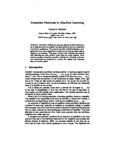
the two parallel hyperplanes separates the two classes (the positive and negative data points) well; on the other hand, the margin between the two hyperplanes is maximised, leading to introduce the regularisation term. Thus, the structural risk minimisation principle is implemented. The final separating hyperlane is selected to be the ‘middle one’ between the above two hyperplanes. Figure 1 (a) shows the geometric interpretation of SVM for a toy example. Figure 1

Geometric interpretation of algorithm: (a) SVM and (b) GEPSVM (see online version for colours) Pos Point Neg Point

wT x  b  1

wT x  b  1

(a)

(b)

Compare with artificial neural network (ANN), one main advantage of SVM is that it attempts to maximise the margin by solving a convex quadratic programming problem (QPP), which obtains an unique global minimum. However, this is also a double-edged sword. The computational complexity of SVM is O (m3), where m is the size of dataset, which means it is difficult to handle the large scale problems (Shao and Deng, 2012a). In addition, the performance of SVM also depends on the optimal parameters selections (Peng, 2011). Different from constructing two parallel hyperplanes in SVM, Mangasarian and Wild (2006) proposed a generalised eigenvalue proximal support vector machine(GEPSVM), which aims at generating two non-parallel hyperplanes such

that each hyperplane is closer to its class and is as far as possible from the other class. A fundamental difference between GEPSVM and SVM is that, GEPSVM solves two generalised eigenvalue problems to obtain two non-parallel hyperplanes, whereas, SVM solves one QPP to obtain one hyperplane. Therefore, GEPSVM works faster than SVM. Experimental results in (Mangasarian and Wild, 2006) showed the effectiveness of GEPSVM on UCI datasets. In addition, GEPSVM is excellent at dealing with the ‘Cross Planes’ datasets. To further improves the generalisation performance of GEPSVM, many modified models (Jayadeva et al., 2007; Shao et al., 2011; Shao and Deng, 2012b; Shao et al., 2012c; Shao et al., 2012d) have been proposed. In this paper, we concern about ensemble learning to improve the generalisation performance of GEPSVM. Ensemble learning is a powerful machine learning paradigm which has exhibited apparent advantages in many applications, such as: medicine (Mangiameli et al., 2004), credit risk evaluation (Yu et al., 2010), bioinformatics (Zhang et al., 2012), and image retrieval (Ling et al., 2006). The main idea behind the ensemble learning is to weigh the individual learners/classifiers, and then combine them, in some way, to obtain a super-learner that outperforms all of them (Rokach, 2010). The last decade has witnessed ensemble learning is very effective learning paradigm (Gao et al., 2010). One key of the successful ensemble is to measure the diversity, which plays an important role in ensemble. To ensemble GEPSVM, we should present the proper diversity measures for individual learners. However, GEPSVM is not sensitive to different weights of the points because it is the proximal classifier. To increase the potential diversity, firstly, we introduce an extra parameter, which make it to give different penalties for different classes. Then, a novel bagging strategy based on GEPSVM is proposed, called EnGEP for short. Experimental results both on artificial and benchmark datasets show that our EnGEP improves the generalisation ability of GEPSVM greatly, and it also reveals the effectiveness of our EnGEP. The paper is organised as follow: Section 2 brief reviews the GEPSVM, Section 3 proposes our EnGEP, Section 4 presents the experimental results from several artificial and the UCI repository, Section 5 draws conclusions.

2

Reviews of GEPSVM

Consider a binary classification problem in the ndimensional real space Rn. We organise the m1 points of Class 1 by matrix X 1  R m1 n and the m2 points of Class −1 by matrix X 2  R m2  n , correspondingly, the m1 outputs of Class 1 by vector y1  R m1 and the m2 outputs of Class 1 by vector y 2  R m2 .

Ensemble learning for generalised eigenvalues proximal support vector machines The goal of GEPSVM (Mangasarian and Wild, 2006) is to find a pair of non-parallel hyperplanes w1T x  b1  0 and w2T x  b2  0,

|| X 1 w1  e1b1 || || ( w1 b1 ) || , || X 2 w2  e2 b1 ||2 || ( w1 b1 ) ||2 2

min

( w1 , b1 )  0

|| X 2 w2  e2 b2 ||2 || ( w2 b2 ) ||2 , ( w2 ,b2 )  0 || X w  e b ||2 || ( w b ) ||2 1 2 1 2 2 2 min

(2)

i 1,2

| wiT x  bi | , || wi ||

|| X 1 w1  e1b1 ||2  || ( w1 b1 ) ||2 , ( w1 , b1 )  0 || X 2 w1  e2 b1 ||2 min

where |  | is the absolute value.

3

GEPSVM ensemble

In this section, to improve the potential diversity of the base classifier, we first propose a novel of GEPSVM by introducing an extra parameter. Then we design an ensemble version of GEPSVM (EnGEP) with bagging strategy.

3.1 Increase diversity of GEPSVM

(4)

From (4) and (5), we can see that GEPSVM set the same  to determine a pair of non-parallel hyperplanes. This may limit the diversity of the two hyperplanes, then it may reduce the range of selected classification function in GEPSVM. To ensemble GEPSVM, we first reformulate GEPSVM by adding a penalty parameter. Then the primal problem becomes: || X 1 w1  e1b1 ||2 1 || ( w1 b1 ) ||2 , ( w1 , b1 )  0 || X 2 w1  e2 b1 ||2 min

and || X 2 w2  e2 b2 ||2  || ( w2 b2 ) ||2 , ( w2 ,b2 )  0 || X 1 w2  e1b2 ||2 min

(5)

where e1 and e2 are both vectors of ones with appropriate dimension. Figure 1(b) shows the geometric interpretation of this formulation for a toy example. In contrast, we also give the geometric interpretation of standard SVM. By introducing the definitions: G  [ X 1 e1 ]T [ X 1 e1 ]   I , H  [ X 2 e2 ]T [ X 2 e2 ],

(6)

L  [ X 2 e2 ]T [ X 2 e2 ]   I , M  [ X 1 e1 ]T [ X 1 e1 ],

(7)

and w  w  z1   1  and z2   2   b1   b2 

(8)

we can reformulate (4) and (5) as z1T Gz1 z T Gz and min T2 2 . T z2  0 z Hz z1 Hz1 2 2

(9)

The above two minimisation problems are exactly Rayleigh quotient (Parlet, 1981) and the global optimal solutions can be readily computed by solving the following two related generalised eigenvalue problems (GEPs) Gz1   Hz1 and Lz2   Mz2 .

(11)

(3)

By introducing a Tikhonov regularisation term that is often used to regularise least squares and mathematical programming problems that reduces the norm of the problem variables (w,b) nonnegative parameter  , we regularise our problem (2)(3) as follows:

z1  0

Class  arg min

2

and

min

x  R n is assigned to class 1 or −1, depending on which of the two hyperplanes is closer to, i.e.,

(1)

where w1  R n , w2  R n , b1  R and b2  R , each hyperplane is generated such that it is closest to the data points of one class and as far as possible from those of the other class. Then, the criteria of GEPSVM yield the following pair of minimisation problems:

275

(10)

The eigenvectors corresponding to smallest eigenvalues are the solution to (4) and (5). Once the solutions (w1b1) and (w2b2) of the problems (4) and (5) are obtained, a new point

(12)

and || X 2 w2  e2 b2 ||2  2 || ( w2 b2 ) ||2 , ( w2 ,b2 )  0 || X 1 w2  e1b2 ||2 min

(13)

where 1 and  2 are positive parameters.

3.2 Bagging GEPSVM In this subsection, we present a novel bagging GEPSVM classifier, called EnGEP. Bagging, short for bootstrap aggregating, is a simple but effective technology for constructing an ensemble of classifier (Rokach, 2010). The idea of bagging GEPSVM is simple and appealing: combines the outputs of diversified base GEPSVMs into a single decision based on bootstrap resample strategy. The bagging engine for our EnGEP is illustrated in Figure 2. In order to obtain the diversity of datasets in bagging, firstly, we employ bootstrap resample strategy to generate different training datasets X ' drawn uniformly with replacement from the original training datasets X . Subsequently, a single GEPSVM is built with the new training datasets X ' . Thus, single GEPSVM can be defined by a pair of non-parallel hyperplanes. Finally, the composite bagged classifier returns the class with the largest votes. Figure 3 presents the pseudo-code of our EnGEP. The EnGEP receives a base leaner LGEP which is used for training all new resampled datasets constructed during every iterations t=1,…T, where T is the ensemble size. In order to

276

W. Chen et al.

classify a new point, single GEPSVM classifier returns its prediction, and then EnGEP fuses them for finally decision (Figure 3). Figure 2

Bagging engine for EnGEP (see online version for colours)

Figure 4

Input: x (a point to be classified). Initialize: Initializes binary class votes C1  0, C1  0 Bagging predicting: 1: Do For t  1, , T

Original Dataset

Validation Dataset

Training Dataset

Algorithm 2: EnGEP predicting

2:

Get predicted class from M t : votet  M t (x)

3:

Increase C1 or C1 by 1 according to votet

4: End For

Testing Dataset

Output: y  arg max(Ci ) i 1, 1

(the class y labeled with the largest votes) Construct new dataset

Resample Algorithm

Set X 1'

Set X 2'

Set X t'

Figure 5 Set X T'

M1

M2

Mt

1: Do For i  1,  , N

MT

Majority voting

Figure 3

Input : X (a set of points to be resampled) d (the resampled weights of points) Initialize: Compute the CDF of d

Training base classifier

Prediction

Algorithm 3: resample

Cumu (i )  Cumu (i  1)  d i , where Cumu (i ) means CDF values, and Cumu (0)  0 3: End For

2:

Resample: Construct new points X   (x 1 ,  , x N ) 1: Do For i  1,  , N

Ensemble classifier

Algorithm 1: EnGEP training

2:

Generate uniform random number r  rand ()

3: 4:

Using BinarySearch to find new point x i min  1, max  N (min max is the index of X )

5:

While (Cumu (min)  r and max  min)

Input : LGEP (base GEPSVM learner), T (number of iterations),

6:

mid  int((min  max) / 2)

X (original training datasets), N (datasets size).

7:

If (Cumu ( mid )  r ) min  mid  1

8: 9:

Else max  mid  1 End If

Bagging training: 1: Do For t  1,  , T (t ) Set the resampled weights d i  1 N

10:

End While

2:

11:

Construct new bootstrap points X 

Add new point xi  xmin

3:

12: End For

using the Resample Algorithm 4:

Train classifer M t using LGEP with X 

Out put: X  (a set of new resampled points)

5: End For Output: M (a series of base GEPSVM learners )

For the purpose of implementing the bootstrap resampling in Figure 3, we first compute the CDF (cumulative distribution function) of the resampled weights d=(d1,d2,…,dN) where di  N1 . Then we use a uniform random number r  [0 1] to select a new point by binary search of the CDF. The resample pseudo-code is described in Figure 4. Note that since bootstrap resampling with replacement is used, points in the original datasets X may appear more than once or none in new datasets X ' . A point in X has probability 1  (1  m) m of being selected at least once in the m times are randomly selected from the training datasets (Chen et al., 2009). When m is large enough, the probability is approximate to 63.2%. This perturbation causes different certain diversities of resampled dataset, which makes classifiers diverse.

4

Experimental results

In order to evaluate our EnGEP, we investigate its classification performance on both artificial and UCI benchmark data sets. In experiments, we focus on the comparison between our EnGEP and some state-of-the-art classifiers, including SVM (Chang and Lin, 2011), GEPSVM (Mangasarian and Wild, 2006) and EnSVM (Ensemble version of SVM). All the classifiers are implemented in MATLAB 7.0 (http://www.mathworks.com) environment on a PC with Intel P4 processor (2.9GHz) with 1 GB RAM. In our experiments, we employ libsvm (Chang and Lin, 2011) to implement the SVM and EnSVM. GEPSVM and our EnGEP are implemented using simple MATLAB functions like ‘eig’, respectively. As for the problem of selecting parameters for SVM and GEPSVM, we employ standard 10-fold cross-validation technique. Furthermore, all parameters for SVM and GEPSVM are selected from the set {28 , , 28 } . For EnSVM, the

Ensemble learning for generalised eigenvalues proximal support vector machines parameter C is configure as C=1. For En-GEP, the parameters 1 and  2 are configure as follow strategy: when

Ratio 

size ( X1 ) size ( X 2 )

 1 , set 1  Ratio and  2  1 , else when

Ratio  1 , set 1  1 and  2  Ratio . The parameter of RBF kernel is configure as q=1 for both.

Figure 7

277

Results of nonlinear SVM, GEPSVM, EnSVM and EnGEP on Ripley’s synthetic dataset, in which the positive and negative points are denoted as “+” and “×”, and the mis-classified points are marked by extra circles: (a) SVM, (b) GEPSVM, (c) EnSVM and (d) EnGEP (see online version for colours)

4.1 Evaluation measures Generally, the performance of classifiers is typically evaluated by using accuracy. However, this is not for imbalanced data or unequal error cost problems (Chawla et al., 2002). To evaluate our EnGEP, we consider some more appropriate metrics than accuracy, including sensitivity, specificity, and G-mean. For a binary classification problem (Zhou and Lai, 2009), each point x  R1 n is mapped to one label of the class set {+1,-1} (positive or negative class). Let the symbols {+1,-1} represent the prediction of a classifier and, for a point x the four possible outcomes can be illustrate with a confusion matrix (Figure 6). The columns are the predicted class and the rows are the actual class. In the confusion matrix, TN is the number of negative points correctly classified, FP is the number of negative points incorrectly classified as positive, FN is the number of positive points incorrectly classified as negative and TP is the number of positive points correctly classified. In our experiment, we use four common performance measures associated with classifier, defined as TP TN , Specificity(Spe)= , TP  FP TN  FN TP  TN Accuracy(Acc) = , G-mean  Sen  Spe . TP  FP  TN  FN

(a)

Sensitivity(Sen) 

Figure 6

(b)

Confusion matrix (Chawla et al., 2002) (see online version for colours)

Actual class

Predicted class -1

+1

-1

TN

FP

+1

FN

TP

(c)

4.2 Toy examples In this subsection, we give an artificial-generated Ripley’s synthetic datasets (Ripley, 2008) to show the performance of our EnGEP. The Ripley’s synthetic dataset includes 250 training points and 1000 test points. Figure 7(a–d) show the learning results of SVM, GEPSVM, EnSVM and our EnGEP with the RBF kernel ( K ( x, x)  exp(  || x  x ||2 ) ). It can be seen that our EnGEP obtains the more appropriate surface than the others. This indicates that our EnGEP successfully describe the two classes of points. From Figure 7, we also can see that our EnGEP obtains the best accuracy.

(d)

W. Chen et al.

278

others for the most cases according to the W-T-L summarisation, specifically significantly enhance the performance of GEPSVM.

4.3 Benchmark datasets Further, in order to compare our EnGEP with SVM, GEPSVM and EnSVM, we choose nine data sets from UCI machine learning repository (http://www.ics.uci.edu/~mlear

Table 1

-n/MLRepository.html). Table 1 gives the characteristics of these data sets. They are varied in characteristics with different numbers of points and features. For each data set, four different classifiers was trained and tested by ten crossvalidation methods. Furthermore, in the experiments we only consider the Gaussian kernels for these classifiers. Points to one class. With the help of ensemble technology, the accuracy and G-mean are both improved significantly on most of datasets. A win-tie-loss (W-T-L) summarisation based on mean is also attached at the bottom of Table 2 and 3. It can be clearly seen that, from Heartstatlog to CMC, the proposed EnGEP obtain the best classification performance than the Table 2

Description of UCI datasets

Dataset

Size

Features

Class

Heartstatlog

131

10

43/88

Sonar

208

60

97/111

Monks3

432

7

216/216

Housevotes

435

16

267/168

Australian

690

14

307/383

TicTacToe

958

27

626/332

Diabetics

768

8

268/500

Heartc

303

14

139/146

CMC

1473

9

1140/333

Performance in terms of Sen and Sep on benchmark datasets. SVM

Dataset

GEPSVM

EnSVM

EnGEP

Sen

Spe

Sen

Spe

Sen

Spe

Sen

Spe

Heartstatlog

74.31±9.48

83.73±5.82

78.36±8.61

81.77±9.05

84.54±12.48

82.45±6.38

88.25±2.93

84.19±2.15

Sonar

93.31±9.73

95.65±12.19

92.31±4.53

94.29±5.28

96.06±5.19

95.31±6.36

98.36±2.43

97.17±5.28

Monks3

69.80±4.71

65.41±8.99

62.80±14.71

58.37±6.57

56.75±9.31

47.38±8.17

71.33±8.76

63.87±5.39 92.83±5.62

Housevotes

89.24±8.34

94.51±6.38

95.32±6.42

90.33±3.43

94.81±5.71

95.74±2.79

97.95±3.29

Australian

75.28±5.51

79.30±8.80

0.00±0.00

68.51±4.90

85.22±6.25

68.18±4.09

79.16±2.79

84.14±3.27

TicTacToe

100.00±0.00

100.00±0.00

92.16±2.79

89.67±6.59

98.03±3.10

99.08±0.59

99.84±0.47

99.65±0.52

Diabetics

75.97±4.41

0.00±0.00

78.21±3.39

0.00±0.00

82.89±3.61

79.42±10.60

81.75±6.83

86.47±4.01

Heartc

83.14±4.58

80.13±4.48

79.48±8.31

80.35±4.52

86.74±4.61

85.16±3.77

88.93±4.63

84.55±5.84

CMC

80.13±3.24

0.00±0.00

0.00±0.00

82.51±1.59

83.68±1.65

69.17±9.53

81.20±3.95

59.28±12.72

W-T-C

8-0-1

6-0-3

9-0-0

8-0-1

6-0-3

6-0-3

Table 3

Performance in terms of Acc and G-mean on benchmark datasets.

Dataset

SVM

GEPSVM

EnSVM

EnGEP

Acc

G-mean

Acc

G-mean

Acc

G-mean

Acc

G-mean

Heartstatlog

79.12±5.42

67.13±3.92

80.31±6.21

75.13±5.14

82.56±3.40

83.05±4.67

84.13±4.12

85.38±6.55

Sonar

93.16±6.19

89.19±6.30

92.13±5.21

87.31±4.85

95.49±3.56

95.58±3.55

98.13±1.29

97.33±2.15

Monks3

80.33±4.16

54.16±8.12

76.33±7.21

45.13±9.35

79.26±5.50

48.33±10.98

78.91±6.21

50.24±11.26

Housevotes

93.11±3.13

90.28±5.02

94.21±4.65

91.60±3.72

95.60±1.68

95.20±2.58

94.13±1.68

93.17±3.32

Australian

79.13±2.32

62.11±4.28

68.51±4.90

0.00±0.00

82.40±1.68

71.21±5.38

84.60±2.88

74.73±1.55

TicTacToe

100.00±0.00

100.00±0.00

95.31±3.52

90.11±4.38

98.85±0.59

98.54±1.38

99.48±0.21

99.29±0.13

Diabetics

75.97±4.41

0.00±0.00

78.21±3.39

0.00±0.00

82.22±2.93

80.92±5.65

84.41±2.95

83.06±3.69

Heartc

85.37±5.18

79.65±6.32

84.38±2.21

79.12±2.60

85.79±2.95

86.78±4.48

86.12±3.77

85.21±6.18

CMC

80.13±3.24

0.00±0.00

82.51±1.59

0.00±0.00

83.90±1.18

75.36±9.92

83.16±1.82

61.28±10.12

W-T-C

7-0-2

7-0-2

8-0-1

9-0-0

6-0-3

6-0-3

Ensemble learning for generalised eigenvalues proximal support vector machines Table 2 and 3 summarise the results of these classifiers, including the average cross-validation Sen, Spe, Acc, and G-mean, where the best one is shown by bold figures. From Table 3, we are surprised to find that the G-mean values of SVM and GEPSVM equal to 0 in some datasets, such as Australian, Diabetics and CMC. Combine with Table 2, we can see some sensitivity or specificity values are equal to 0, which mean that the classifier maps all

5

Conclusions

In this paper, we have proposed ensemble GEPSVM for binary classification. To increase the diversity of our ensemble classifier, we introduce an extra parameter to give different penalties for two non-hyperplanes determined by GEPSVM. Further, we design a novel bagging strategy to ensemble GEPSVM with additional parameters. Experimental results both on artificial and benchmark datasets show that our EnGEP improved the generalisation performance of GEPSVM greatly, and it also reveals the effectiveness of our EnGEP. However, the proximal classifiers such as GEPSVM are not sensitive to different weights of the points. So, to further enhance of diversity the proximal classifiers is our future work.

Acknowledgement This work is supported by the National Natural Science Foundation of China (No.10971223, No.11071252 and No. 11201426), the Zhejiang Provincial Natural Science Foundation of China (No.LQ12A01020, No. LQ13F030010 and No.Y1100629) and the Science and Technology Foundation of Department of Education of Zhejiang Province (No.Y201225179).

References Chang, C. and Lin, C. (2011) ‘LIBSVM: a library for support vector machines’, ACM Transactions on Intelligent Systems and Technology, Vol. 3, pp.1–27. Chawla, N., Bowyer, K., Hall, L. and Kegelmeyer, P. (2002) ‘Smote: synthetic minority over-sampling technique’, Journal of Artificial Intelligence Research, Vol. 16, pp.321–357. Chen, S., Wang, W. and van Zuylen, H. (2009) ‘Construct support vector machine ensemble to detect traffic incident’, Expert Systems with Applications, Vol. 36, No. 8, pp.10976–10986. Chiraz, B.O.Z., Feriel, B.F. and Mohamed, B.A. (2011) ‘An intelligent tool for syntactic annotation of Arabic corpora’, International Journal of Computer Applications in Technology, Vol. 40, No. 4, pp.227–237. Gao, C., Sang, N. and Tang, Q. (2010) ‘On selection and combination of weak learners in adaboost’, Pattern Recognition Letters, Vol. 31, No. 9, pp.991–1001. Jayadeva, Khemchandani, R. and Chandra, S. (2007) ‘Twin support vector machines for pattern classification’, IEEE Transactions on Pattern Analysis and Machine Intelligence, Vol. 29, No. 5, pp.905–910. Keiko, M. and Setsuya, K. (2011) ‘Optimising of support plans for new graduate employment market using reinforcement learning’, International Journal of Computer Applications in Technology, Vol. 40, No. 4, pp.254–264.

279

Ling, C.X., Sheng, V.S. and Yang, Q. (2006) ‘Test strategies for cost-sensitive decision trees’, IEEE Transactions on Knowledge and Data Engineering, Vol. 18, No. 8, pp.1055–1067. Mangasarian, O.L. and Wild, E.W. (2006) ‘Multisurface proximal support vector machine classification via generalized eigenvalues’, IEEE Transactions on Pattern Analysis and Machine Intelligence, Vol. 28, No. 1, pp.69–74. Mangiameli, P., West, D. and Rampal, R. (2004) ‘Model selection for medical diagnosis decision support systems’, Decision Support Systems, Vol. 36, No. 3, pp.247–259. Ma, J., Wang, F., Jia, Z. and Wei, W. (2011) ‘Using support vector machine for characteristics prediction of hydraulic valve’, International Journal of Computer Applications in Technology, Vol. 41, Nos. 3/4, pp.287–295. Parlet, B.N. (1981) ‘General Rayleigh quotient iteration’, SIAM Journal on Numerical Analysis, Vol. 18, No. 5, pp.839–843. Peng, X. (2011) ‘TPMSVM: a novel twin parametric margin support vector machine for pattern recognition’, Pattern Recognition, Vol. 44, Nos. 10/11, pp.2678–2692. Ripley, B. (2008) Pattern Recognition and Neural Networks, Cambridge University Press. Rokach, L. (2010) Pattern Classification Using Ensemble Methods (Series in Machine Perception and Artificial Intelligence), World Scientific. Sang, S., Liu, M., Liu, J. and An, Q. (2010) ‘A new approach for texture classification in CBIR’, International Journal of Computer Applications in Technology, Vol. 38, Nos. 1/2/3, pp.34–39. Shao, Y.H., Zhang, C.H., Wang, X.B. and Deng, N.Y. (2011) ‘Improvements on twin support vector machines’, IEEE Transactions on Neural Networks, Vol. 22, No. 6, pp.962–968. Shao, Y.H. and Deng, N.Y. (2012a) ‘A coordinate descent margin based-twin support vector machine for classification’, Neural Networks, Vol. 25, pp.114–121. Shao, Y.H. and Deng, N.Y. (2012b) ‘A novel margin-based twin support vector machine with unity norm hyperplanes’, Neural Computing and Applications, OI: 10.1007/s00521-012-0894-5. Shao, Y.H., Deng, N.Y. and Yang, Z.M. (2012c) ‘Least squares recursive projection twin support vector machine for classification’, Pattern Recognition, Vol. 45, No. 6, pp.2299–2307. Shao, Y.H., Deng, N.Y., Yang, Z.M., Chen, W.J. and Wang, Z. (2012d) ‘Probabilistic outputs for twin support vector machines’, Knowledge-Based Systems, Vol. 33, pp.145–151. Singh, Y., Kaur, A. and Malhotra, R. (2009) ‘Comparative analysis of regression and machine learning methods for predicting fault proneness models’, International Journal of Computer Applications in Technology, Vol. 35, Nos. 2/3/4, pp.183–193. Vapnik, V. (1998) Statistical Learning Theory, Wiley. Yu, L., Yue, W., Wang, S. and Lai, K.K. (2010) ‘Support vector machine based multiagent ensemble learning for credit risk evaluation’, Expert Systems with Applications, Vol. 37, No. 2, pp.1351–1360. Yu, W., Jiang, X. and Xiong, B. (2009) ‘Data preparation for samplebased face detection’, International Journal of Computer Applications in Technology, Vol. 35, No. 1, pp.10–22. Zhang, Y., Zhang, D., Mi, G., Ma, D., Li, G., Guo, Y., Li, M. and Zhu, M. (2012) ‘Using ensemble methods to deal with imbalanced data in predicting protein protein interactions’, Computational Biology and Chemistry, Vol. 36, pp.36–41. Zhou, L. and Lai, K. (2009) ‘Benchmarking binary classification models on data sets with different degrees of imbalance’, Frontiers of Computer Science in China, Vol. 3, No. 2, pp.205–216.