An Ensemble Approach for Incremental Learning in Nonstationary Environments Michael D. Muhlbaier and Robi Polikar* Signal Processing and Pattern Recognition laboratory Electrical and Computer Engineering, Rowan University, Glassboro, NJ 08028 USA
[email protected],
[email protected]
Abstract. We describe an ensemble of classifiers based algorithm for incremental learning in nonstationary environments. In this formulation, we assume that the learner is presented with a series of training datasets, each of which is drawn from a different snapshot of a distribution that is drifting at an unknown rate. Furthermore, we assume that the algorithm must learn the new environment in an incremental manner, that is, without having access to previously available data. Instead of a time window over incoming instances, or an aged based forgetting – as used by most ensemble based nonstationary learning algorithms – a strategic weighting mechanism is employed that tracks the classifiers’ performances over drifting environments to determine appropriate voting weights. Specifically, the proposed approach generates a single classifier for each dataset that becomes available, and then combines them through a dynamically modified weighted majority voting, where the voting weights themselves are computed as weighted averages of classifiers’ individual performances over all environments. We describe the implementation details of this approach, as well as its initial results on simulated non-stationary environments. Keywords: Nonstationary environment, concept drift, Learn++.NSE.
1 Introduction The problem of learning in nonstationary environments (NSE) has traditionally received much less attention than its stationary counterpart. It is perhaps due to inherent difficulty of the problem: after all, machine learning algorithms require a formal and precise definition of the problem, and in this case, it is even difficult to define the problem: what exactly is a nonstationary environment? Informally, it refers to the variation of the underlying data distribution that defines the concept to be learned: the environment subsequently provides new data, for which the input/output mapping (decision boundary) is different than those of the previous datasets. Early work in NSE learning, also known as concept drift, have concentrated on formalizing exactly what kind of drift and/or how fast of a drift can be learned [1-4]. Therein lies the difficulty with this problem; change can be slow or fast, abrupt or gradual, random or systematic, cyclical, expanding or contracting in the feature space. *
Corresponding author.
M. Haindl, J. Kittler, and F. Roli (Eds.): MCS 2007, LNCS 4472, pp. 490–500, 2007. © Springer-Verlag Berlin Heidelberg 2007
An Ensemble Approach for Incremental Learning in Nonstationary Environments
491
Several approaches have been proposed for various combinations of such changes, which typically include a mechanism to (i) detect the drift and/or its magnitude; (ii) learn the change in the environment; and/or (iii) forget what is no longer relevant. Many algorithms specifically designed for concept drift are generally based in part on the ideas used in FLORA [3]: use a timing window (fixed or variable) to choose a block of (new) instances as they come in, and then train a new classifier. The window size can be increased or decreased depending on how fast the environment is changing. Of course, such algorithms have a built-in forgetting mechanism with the implicit assumption that those instances that fall outside of the window are no longer relevant, and the information carried by them can be forgotten. Other approaches try to detect when a substantial change has occurred (novelty detection), and then update the classifier [5-8], or find the extreme examples that carry most relevant and novel information to train a classifier (partial instance memory) [9]; still others detect and purge those instances that no longer carry relevant information, and train a new classifier with the remaining block of data [10]. A different group of approaches treat the nonstationary learning as a prediction problem, and use appropriate classification (e.g., PNN) [11] or tracking algorithms (such as Kalman filters) [12]. More recently, ensemble based approaches have also been proposed. As reviewed by Kuncheva in [13], such algorithms typically fall into one of the following categories: (i) dynamic combiners where, for a previously trained fixed ensemble, the combination rule is changed to track the concept drift, e.g., weighted majority voting or Winnow based algorithms [14]; (ii) algorithms that use the new training to update an online learner or all members of an ensemble, e.g. online boosting [15]; and (iii) algorithms that add new ensemble members [16] and/or replace the least contributing member of an ensemble with a classifier trained on new data [17,18]. In this paper we propose an alternative formulation, Learn++.NSE, built upon our previously introduced incremental learning algorithm Learn++ [19], by suitably modifying it for nonstationary environments. Learn++.NSE does not completely fit into any of the above categories, but rather combines ideas from each. It does use new data to create new ensemble members, and it also adjusts the combination rule by dynamically modifying voting weights. It does not use a timing window, or any of the previously seen data (hence an incremental learning approach), and it does not discard old classifiers, in case old classifiers become relevant again in the future. It simply reweighs them based on their predicted expertise on the current environment. It is reasonable to question whether there is need for yet another ensemble based algorithm for nonstationary learning, in particular considering that we make no claim on the superiority of Learn++.NSE over any of the other algorithms – ensemble based or otherwise. In the spirit of the no-free-lunch theorem, we believe that no single algorithm can outperform all others on all applications, that the success depends much on the match of the characteristics of the algorithm with those of the problem, and therefore it is best to have access to a toolbox of algorithms each with its own particular strengths and weaknesses. Considering the differences of Learn++.NSE mentioned above, along with the promising initial results and outcomes discussed later in this paper, we believe that Learn++.NSE can be a beneficial alternative on a variety of nonstationary learning scenarios. The algorithm is described in detail in Section 2,
492
M.D. Muhlbaier and R. Polikar
followed by a description of our simulation tests and results in Section 3. Specific nonstationary environment scenarios in which the algorithm is expected to be particularly useful are discussed in Section 4.
2 Learn++.NSE Learn++.NSE uses a similar structural framework as Learn++: incrementally build an ensemble of classifiers from new data that are combined by weighted majority voting, and the existing ensemble decides on the contribution of each successive classifier. There are a number of differences, however, instituted for suitably modifying the algorithm for nonstationary environments. In summary, we assume that each new dataset represents a new snapshot of the environment. The amount of change in the environment since the previous dataset may be minor or substantial, and is tracked by the performance of the existing ensemble on the current dataset. Learn++.NSE creates a single classifier for each dataset that becomes available from the new environment, and a weighted performance measure (based on its error) is computed for each classifier on each environment it has experienced. Each performance measure represents the expertise of that classifier on a particular snapshot of the environment. These performance measures are then averaged using a nonlinear (sigmoidal) function, giving higher weights to the performances of the classifier on the more recent environments. At any time, the classifiers can be combined through weighted majority voting, using the most recent averaged weights, to obtain the final hypothesis. In Learn++.NSE, the change in the environment is tracked both by addition of new classifiers, as well as the voting weights of existing classifiers, and no classifier is ever discarded. If cyclical drift makes earlier classifiers once again relevant, the algorithm recognizes this change, and assigns higher weights to earlier classifiers. The algorithm is described in detail below, with its pseudocode given in Fig. 1. We assume that an oracle provides us with a training dataset at certain intervals, (not necessarily uniform). At each interval, the distribution from which the oracle draws the training data changes in some manner and rate, also unknown to us. The training dataset Dt of cardinality mt at time t provides us with a snapshot of the then current environment. Learn++.NSE generates one classifier for each such new dataset that becomes available. To do so, the algorithm first evaluates the classification accuracy of the currently available composite hypothesis Ht-1 on the newly available data Dt. Ht-1, obtained by the weighted majority voting of all classifiers generated during the previous t-1 iterations, represents the existing ensemble’s knowledge of the environment. The error of the composite hypothesis Et is computed as a simple ratio of the correctly identified instances of the new dataset. We demand that this error be less that a threshold, say ½, to ensure that it has a meaningful classification capacity. For this selection of the threshold, we normalize the error so that the normalized error Bt remains between 0 and 1 (Step 1 inside the Do loop). We then update a set of weights for each instance, that is normally initialized to be uniform (1/mt ): the weights of the instances misclassified by the ensemble are reduced by a factor of Bt . The weights are then normalized to obtain a distribution Dt (step 2).
An Ensemble Approach for Incremental Learning in Nonstationary Environments
493
Input: For each dataset Dt t=1,2,…representing a new environment • Sequence of i=1,…,mt instances xi with labels yi ∈ Y = {1,…,c} • Supervised learning algorithm BaseClassifier. Do for t=1,2,… If t=1 Initialize
D1 ( i ) = w1 ( i ) = 1/ m1 , ∀i, skip to step 3.
(1)
1. Compute error of existing ensemble on new data m E t = ∑ i =1 (1 mt ) ⋅ ced H t −1 ( xi ) ≠ yi fgh t
Normalize error B
t
(2)
= E t (1 − E t )
(3)
2. Update instance weights
t t −1 1 ⎪⎧ B , H ( xi ) = yi w = t ×⎨ m ⎩⎪1, otherwise t i
Set
D =w t
t
(4)
mt
∑w
t i
i =1
so that Dk is a distribution.
(5)
3. Call BaseClassifier with Dt, obtain ht : X Æ Y 4. Evaluate all existing classifiers on new dataset Dt
ε kt = ∑ i =1 D t ( i ) ⋅ ce hk ( xi ) ≠ yi fh, mt
If
ε
> 1 2 , generate a new ht. If ε
t k =t
β =ε t k
(1 − ε ) ,
t k
t k
for k = 1,..., t t k 1 2 , set ε = 1 2 t k
for k = 1,..., t
(7) th
5. Compute a weighted sum of all normalized errors for k classifier hk
(
ωkt = 1 1 + e − a(t − k −b)
),
ωkt = ωkt
∑
t −k j =0
ωkt − j
(8)
t −k
β kt = ∑ ωkt − j β kt − j , for k = 1,..., t
(9)
j =0
6. Calculate classifier voting weights
Wkt = log (1 β kt ) , for k = 1,..., t
(10)
7. Obtain the composite hypothesis as the current final hypothesis
H t ( xi ) = arg max ∑ k Wkt ⋅ce hk ( xi ) = c fh
(11)
c
Fig. 1. The pseudocode of the algorithm Learn++.NSE
The algorithm then calls the BaseClassifier and asks it to create the tth classifier ht using data drawn from the current training dataset Dt provided by the oracle (step 3). All classifiers generated thus far hk, k=1,...,t are then evaluated on the current dataset, by computing their weighted error (Equation 6, step 4). Note that at current time step t, we
494
M.D. Muhlbaier and R. Polikar
now have t error measures, one for each classifier generated thus far. Hence the error term εkt represents the error of the kth classifier hk at the tth time step. The errors are again assumed to be less than ½. Here, we make a distinction: if the error of the most recent classifier (on its native training set) is greater than ½, then we discard that classifier and generate a new one. For any of the other (older) classifiers, if its error is greater than ½, it is set to ½. This effectively sets the normalized error of that classifier at that time step to 1, which in turn removes all of its voting power later during the weighted majority voting. Note that unlike AdaBoost and similar algorithms that use such an error threshold, Learn++.NSE does not abort, nor does it throw away (the previously generated) classifiers when their error exceeds ½. This is because, it is not unreasonable for a classifier to perform poorly if the environment has changed drastically since it was created, and furthermore, it does not mean that this classifier will never be useful again in the future. Should the environment goes through a cyclical change and becomes similar to the time when the classifier in question was generated, its error will then be less than ½ , and it will contribute to the current decision of the ensemble. In order to combine the classifiers, however, we need one weight for each, even though the algorithm maintains a set of t such error measures εkt for each classifier k=1,…,t. The error measures are therefore combined through a weighted averaging (step 5). The weighting is done through a sigmoid function (Equation 8), which gives a large weight to errors on most recent environments, and less to errors on older environments. We emphasize, however, that this process does not give less weight to old classifiers. It is their error on old environments that is weighted less. Therefore, a classifier generated long time ago can in fact receive a large voting weight, if its error on the recent environments is low. The errors so weighted as described above are then combined to obtain a weighted average error (Eq. 9). The logarithm of the inverse of this weighted error average then constitutes the final voting weight Wkt for classifier k at time instant t (Step 6, Eq. 10). Finally all classifiers are combined through weighted majority voting (Step 7, Eq. 11).
3 Experiments and Results Two experiments were designed to test the ability of the algorithm to track a nonstationary environment. In both experiments, data was drawn from Gaussian distributions so that the optimal Bayes error could be computed and compared – at each time step – against the Learn++.NSE ensemble as well as single classifier performances. Naive Bayes was used as the base classifier in all experiments. In the first experiment, conceptually illustrated in Fig. 2, the distributions for two of the three classes were moved in a concept drift scenario, where both the means and the variances of the distributions were changed. In fact, the distribution of one class has completely replaced the other. The entire change was completed in 50 time steps, however, in each case, we allowed the algorithm to see very little of the environment: a mere 20 samples per class. The distribution for the third class left unchanged. We then tracked the performance of the Learn++.NSE ensemble, a single classifier, and the Bayes classifier, at each time step. Figure 3 shows four independent trials of the percent classification performances on the entire feature space, calculated with
An Ensemble Approach for Incremental Learning in Nonstationary Environments
y 8
495
Class 1 [5 8 3 0.5]
Class 1 new [8 5 1 1]
5
Class 2 [8 4 1 1]
Class 3 (no change) [ 5 5 1 1]
2
[ μx μy σx σy ]
[8 5 2 2] Class 2 new
Path of drift
x
8
5
Fig. 2. Concept drift simulation – 3-class experiment. Classes 1 and 2 move and change variance. 1
1
0.95
0.95
% performance on the entire feature space
0.9
0.9
0.85 0.85 0.8 0.8 0.75 0.75
0.7
0.7
0.65
0
10
20
30
40
50
0.65
1
1
0.95
0.95
0.9
0.9
0.85
0.85
0.8
0.8
0.75
0.75
0.7
0.7
0.65
0
10
20
++
Learn .NSE
30
40
50
0.65
0
10
20
30
0
10
20
30
Single Classifier
Bayes Classifier
40
50
40
50
Time step
Fig. 3. Comparative performances on four independent single trials
respect to individual instances’ probability of occurrence (to prevent instances away from decision boundaries artificially increasing the performance). Several interesting observations can be made. First, all four performance trends indicate that the Learn++.NSE tracks the Bayes classifier very closely, and as expected, it has smaller performance variance than the single classifier.
496
M.D. Muhlbaier and R. Polikar
Second, the ensemble performance is, in general, better than the single classifier, and more closely follows the Bayes classifier. This is important since a single Naïve Bayes classifier tested on the most recent data on which it was trained would normally be expected to do very well. The ensemble is using its combined knowledge from all training sessions to correctly identify those areas that have changed due to concept drift as well as those that have not changed. Third, the performance gap between the ensemble and the single classifier appear to be widening in time, in favour of the ensemble. That is, the performances of single classifier and Learn++.NSE start similar, but in time the ensemble increasingly outperforms the single classifier despite occasional good single classifier performances. Since the large variance in the single classifier performance makes it difficult to determine the validity of such a claim, we looked at the average performance of 100 independent trials of the same experiment. Performance results in Figure 4 indicate that the Learn++.NSE ensemble increasingly and significantly outperforms the single classifier. Finally, note that what appears to look like an overall performance decline (from 90% to 70%-80% range) in Fig.2 and Fig. 4 is irrelevant for our purposes. Such a decline merely indicates that the underlying classification problem is getting increasingly difficult in time (see Fig. 2), as evidenced by the declining optimal Bayes classifier performance. We are primarily concerned with how well Learn++.NSE tracks Bayes classifier, as we cannot expect any algorithm to do any better. % performance on the entire feature space
1
Learn++.NSE Singe Classifier Bayes Classifier
0.95
0.9
0.85
0.8
0.75
0.7
0
5
10
15
20
25
30
35
40
45
50
Time step
Fig. 4. Comparative performances - average of 100 independent trials
We have also designed a second, four-class experiment, the non-stationary environment of which was substantially more challenging, including classes switching places, changing variances, drifting in and out of their original distributions in a cyclical manner. Figure 5 provides snapshots of the distributions of four classes c1 ~ c4 at t=0, t=T/3, t=2T/3 and t=T, where T indicates the time of the last environment update. During t=0 to t=T/3, the variances of the class distributions were modified; then the means of the class distributions drifted until t=2T/3, and finally both the variances and means were changed during the last third section of the simulation. There were a total of 120 time steps from t=0 to t=T, during which the distributions briefly returned to the vicinity of their original neighbourhoods twice, before drifting again in other directions. Hence, the design simulated a semi-cyclical non-stationary behaviour.
An Ensemble Approach for Incremental Learning in Nonstationary Environments
0.4 0.4
time = 0
C
1
0.2
time = T/3
C
1
0.2
C
4
0 0
0 0
C
2
10
5
10
5
5
10
0
10 0 0.4
0.4
time = 2T/3
0.2
time = T
C 0.2
C
1
1
4
2
2
C
C
C
0 0
4
2
3
5
C
C
C
C
3
C
4
0 0
C
C
3
3
10
5
10
5
5
5 10
497
10
0
0
Fig. 5. The snapshots of the drifting distributions at four time steps
% Classification performance on the entire feature space
1
0.98
Learn++.NS Single Classifier Bayes Classifier
Variances of the class distributions drift
0.96
0.94
0.92
0.9
0.88
0.86
Class distributions drift from one location to another
0.84
0.82
0
20
40
60
Both class location drift and variance drift
80
100
Time step each indicating a different environment
Fig. 6. Classification performance results on the second experiment
120
498
M.D. Muhlbaier and R. Polikar
The classification performance results of Learn++.NSE, single classifier and the Bayes classifier are shown in Figure 6, where all performances are averages of 100 independent trials. Once again, the ensemble was able to track the Bayes classifier much closer than the single classifier, despite the convoluted changes in the environment. The ensemble performance was also significantly better than the single Naïve Bayes classifier at the 95% level for all t>5 steps.
4 Conclusions and Discussions We described an ensemble based algorithm for nonstationary environments. The algorithm creates a single classifier for each dataset that becomes available, and keeps a record of the performance of each classifier on all environments throughout the training. The classifiers are then combined through a modified dynamically weighted majority voting, where the voting weights are determined as a measure of each classifier’s performance on the current environment, weighted along with the performances on previous environments. All classifiers are retained, which allows the previously generated classifiers to make significant contributions to the ensemble decision, if such classifiers provide relevant information for the current environment. The algorithm has many characteristics that are deemed desirable for online learners [13]: (i) the algorithm learns from only single pass of each dataset, without revisiting them. This property of the algorithm is inherited from its predecessor Learn++, as it was designed to learn incrementally without requiring access to previously seen data; (ii) the algorithm has a relatively small computational complexity that is linear in the number of datasets, or even possibly in the data size, depending on the base classifier (since it can be used with any supervised classifier); (iii) the algorithm possesses any-time-learning capability, i.e., if the algorithm is stopped at time t, the algorithm provides the current best representation of the environment at that time. As mentioned earlier in our justification for another ensemble based nonstationary learning algorithm, the success of any algorithm depends much on how well its characteristics match those of the problem. It is therefore appropriate, and in fact necessary, to establish what such characteristics are for Learn++.NSE. Specifically, when would we expect this algorithm to do well? The structure of Learn++.NSE makes it particularly useful if the nonstationary environment provides a sequence of relatively small data, that by itself is not sufficient to adequately represent the current state of the environment. Then, a single classifier generated with such data would not be able to appropriately characterize the decision boundary. Only a subset of classes being represented in each dataset is another scenario of nonstationary learning, and the performance of Learn++.NSE on such scenarios is part of our planned future work. The algorithm described here is certainly not fully developed yet, and much work needs to be done. The algorithm, while intuitive, is based on heuristic ideas, and there are no theoretical performance guarantees. This is in part because we have not placed any restrictions on the environment. However, a careful analysis of the algorithm is necessary to determine how it reacts to different scenarios of nonstationary environments, and specifically to different rates of change. Of particular interest is how well the algorithm would be able to track the nonstationary environment, if the environment changed faster, say for example, it made the same total change in T/2 or T/4 time steps rather than in T steps?
An Ensemble Approach for Incremental Learning in Nonstationary Environments
499
While the algorithm is at its early stages of development, its initial performance has been promising, motivating us for further optimization and development. Future efforts will include the above mentioned analysis for tracking / estimating the environment’s rate of change, and the algorithm’s response to such change. Acknowledgments. This material is based upon work supported by the National Science Foundation under Grant No. ECS-0239090.
References [1] Schlimmer, J. C. and Granger, R. H.; Incremental Learning from Noisy Data. Machine Learning 1 (1986) 317-354. [2] Helmbold, D. P. and Long, P. M.; Tracking drifting concepts by minimizing disagreements. Machine Learning 14 (1994) 27-45. [3] Widmer, G. and Kubat, M.; Learning in the presence of concept drift and hidden contexts. Machine Learning 23 (1996) 69-101. [4] Case, J., Jain, S., Kaufmann, S., Sharma, A., and Stephan, F.; Predictive learning models for concept drift. Theoretical Computer Science 268 (2001) 323-349. [5] Liao, Y., Vemuri, V. R., and Pasos, A.; Adaptive anomaly detection with evolving connectionist systems. Journal of Network and Computer Applications 30 (2007) 60-80. [6] Castillo, G., Gama, J., and Medas, P.; Adaptation to Drifting Concepts. Progress in Artificial Intelligence, Lecture Notes in Computer Science 2902 (2003) 279-293. [7] Gama, J., Medas, P., Castillo, G., and Rodrigues, P.; Learning with Drift Detection. Advances in Artificial Intelligence - SBIA 2004, Lecture Notes in Computer Science 3171 (2004) 286-295. [8] Cohen, L., Avrahami-Bakish, G., Last, M., Kandel, A., and Kipersztok, O.; Real-time data mining of non-stationary data streams from sensor networks. Information Fusion In Press, (2007). [9] Maloof, M. A. and Michalski, R. S.; Incremental learning with partial instance memory. Artificial Intelligence 154 (2004) 95-126. [10] Black, M. and Hickey, R.; Learning classification rules for telecom customer call data under concept drift. Soft Computing - A Fusion of Foundations, Methodologies and Applications 8 (2003) 102-108. [11] Rutkowski, L.; Adaptive probabilistic neural networks for pattern classification in timevarying environment. IEEE Transactions on Neural Networks 15 (2004) 811-827. [12] Cheng-Kui, G., Zheng-Ou, W., and Ya-Ming, S.; Encoding a priori information in neural networks to improve its modeling performance under non-stationary environment. International Conference on Machine Learning and Cybernetics (ICMLC 2004) 5 (2004) 30683072. [13] Kuncheva, L. I.; Classifier Ensembles for Changing Environments. Multiple Classifier Systems (MCS 2004), Lecture Notes in Computer Science 3077 (2004) 1-15. [14] Blum, A.; Empirical Support for Winnow and Weighted-Majority Algorithms: Results on a Calendar Scheduling Domain. Machine Learning 26 (1997) 5-23. [15] Oza, N.; Online Ensemble Learning, Ph.D. Dissertation, (2001) University of California, Berkeley. [16] Kyosuke, N., Koichiro, Y., and Takashi, O.; ACE: Adaptive Classifiers-Ensemble System for Concept-Drifting Environments. Multiple Classifier Systems (MCS 2005), Lecture Notes in Computer Science 3541 (2005) 176-185.
500
M.D. Muhlbaier and R. Polikar
[17] Street, W. N. and Kim, Y.; A streaming ensemble algorithm (SEA) for large-scale classification. Seventh ACM SIGKDD International Conference on Knowledge Discovery & Data Mining (KDD-01), (2001) 377-382. [18] Chu, F. and Zaniolo, C.; Fast and Light Boosting for Adaptive Mining of Data Streams. Advances in Knowledge Discovery and Data Mining, Lecture Notes in Computer Science 3056 (2004) 282-292. [19] Polikar, R., Upda, L., Upda, S. S., and Honavar, V.; Learn++: an incremental learning algorithm for supervised neural networks. Systems, Man and Cybernetics, Part C, IEEE Transactions on 31 (2001) 497-508.