Ensemble Neural Network Methods for Satellite-Derived Estimation of Chlorophyll a Wayne H. Slade, Jr.∗ , Richard L. Miller† , Habtom Ressom∗ and Padma Natarajan∗ ∗ University
of Maine Intelligent Systems Laboratory Department of Electrical and Computer Engineering, 113 Barrows Hall, Orono, ME 04469 Email:
[email protected], Telephone: (207) 581–2241, Fax: (207) 581–4531 † NASA, Earth Science Applications Directorate Stennis Space Center, Stennis, MS 39529 Abstract— In this paper, neural network-based methods incorporating ensemble learning techniques are presented that estimate chlorophyll a (chl a) concentration in the coastal waters of the Gulf of Maine (GOM). A dataset was constructed consisting of in situ chl a measurements from the GOM matched with satellite data from the Sea-viewing Wide-Field-of-view Sensor (SeaWiFS). These data were used to develop models using diverse neural network ensembles for estimation of chl a concentration from satellite-retrieved ocean reflectances. Results indicate that the models are able to generalize across geographical and temporal variation, and are resilient to uncertainty such as that introduced by poor atmospheric correction, or radiance contributions from non-chl a components in case 2 waters.
I. I NTRODUCTION Remote sensing of ocean color is a high priority research area for oceanographers, marine biologists, meteorologists, and climatologists for many reasons. For example, NASA’s Earth Science Enterprise seeks to use the unique capabilities of space-borne remote sensing to determine unique information about the Earth’s environment. One particular NASA priority is to improve knowledge of the global biogeochemical cycling of carbon, a key component of which is the contribution from oceanic primary production. While primary production models have improved steadily and significantly over the past decades, imprecision in retrieval of phytoplankton biomass from remotely sensed ocean color remains a primary source of uncertainty in model estimates [1]. This uncertainty lies in the complex bio-optical system linking light and natural waters. Natural waters, both freshwater and ocean, are comprised of many optically active substances (dissolved and particulate) that are highly variable in type and concentration [2], [3]. Typical optically active substances include photosynthetically active pigments, i.e. chlorophyll a (chl a), mineral sediment, detritus, colored dissolved organic matter (CDOM), and the seawater itself. A. Optical Classification of Natural Waters In the open ocean, variations in ocean color are generally due to changes in phytoplankton concentration per unit volume. The primary photosynthetic pigment of phytoplankton, chl a has well studied spectral characteristics [3], [4]. As the concentration of chl a increases, the color of the ocean water gradually shifts from blue to green since chl a absorbs in the blue and red wavelengths selectively [5], [2]. Ocean waters have been loosely classified according to their optical characteristics into two classes, case 1 and case 2. In
case 1 waters, optical properties are dominated by the effects of chlorophyll and associated covariant substances. In contrast, the optical properties of case 2 waters are dominated by the presence of materials which do not covary with chlorophyll [3]. The distinction between case 1 and case 2 waters extends much beyond simply the classification of open ocean or coastal provinces. Waters can be case 2 for many reasons, such as strong remixing due to upwelling events, where optically active substances whose concentrations do not covary with surface chl a concentration are brought near the surface. Morel in 2001 also scrutinizes that case 1 vs. case 2 is not a simple classification. He demonstrates that even case 1 waters do not always behave in the same manner, but rather contain “nuances” that are dependent upon location [6]. Therefore, we propose that neural networks are ideal for implementation of chl a retrieval algorithms for both case 1 and case 2 waters since they do not require a priori information regarding the nature of such “nuances;” given proper input selection and training data, neural network techniques can improve upon current empirical models. B. Sea-viewing Wide Field-of-view Sensor The Sea-viewing Wide Field-of-view Sensor (SeaWiFS) is a multi-spectral ocean color sensor contained on the SeaStar satellite developed by NASA and Orbital Imaging Corporation (OrbImage). SeaWiFS is designed for global and regional study of ocean biology and physics. SeaWiFS scans approximately 15 pole-to-pole orbital swaths of data per day, covering approximately 90% of the ocean surface every two days. Spatial resolution (at nadir) is 1.13 km Local Area Coverage (LAC) and binned for Global Area Coverage (GAC) at 4.5 km. SeaWiFS continuously broadcasts data to ground stations via High Resolution Picture Transmission (HRPT) where the LAC and GAC images are archived. SeaWiFS has superior radiometric sensitivity and signal to noise qualities compared to NASA’s proof-of-concept ocean color mission, the Coastal Zone Color Scanner (CZCS). SeaWiFS has eight spectral bands, six sensing backscattered solar radiance in the visible wavelengths 412, 443, 490, 510, 555, 670 nm, and 2 near-IR channels at 765 and 865 nm. The band at 412 nm is specifically designed for CDOM algorithms. The near-IR bands are designed to facilitate atmospheric correction. The spectral bands are summarized in Table I.
TABLE I S PECTRAL C HANNELS AVAILABLE ON S EAW I FS. Spectral Channel (λ) 412 nm 443 nm 490 nm 510 nm 555 nm 670 nm 765, 865 nm
II. M ETHODS
Designed For CDOM Absorption Chlorophyll absorption Pigment absorption for case 2, optical clarity Chlorophyll absorption Pigments, optical properties, sediment Atmospheric correction, sediment Atmospheric correction, aerosol radiance
C. Chlorophyll a Estimation Algorithms Due to the nature of chl a absorption, band ratios of green to blue reflectances have frequently been used for chl a estimation [5]. Early chl a algorithms used empirical relationships using power-law fits as in Eq. 1, where A and B are empirically determined constants, and Rrs (λ) is the remote sensing reflectance at wavelength λ. [chla ] = A[
Rrs (443) B ] Rrs (550)
(1)
More recently, pigment estimates are based on an empirical algorithms that switch between band ratios, such as the global processing switching (GPs) algorithm for the NASA CZCS. The operational SeaWiFS chl a product, OC4, selects between the maximum of three different band ratios [5]. OC4 version 4 is shown in Eq. 2: chla (µgL−1 ) = 10[a(0)+a(1)R+a(2)R
2
+a(3)R3 +a(4)R4 ]
, (2)
where, a = [0.366, −3.067, 1.930, 0.649, −1.532] i h Rrs (490) Rrs (510) rs (442) > > R = log R Rrs (555) Rrs (555) Rrs (555) . Currently, regional empirical or semi-empirical models exist that are based on case 2 data. The Moderate Resolution Imaging Spectroradiometer (MODIS) sensor utilizes a semiempirical case 2 chl a model [7]. However, it is difficult to account for all of the complexities in case 2 optical environments using empirical algorithms. Other researchers have had success estimating chl a concentration using neural networks, however most have focused on estimation in case 1 environments [8], on hyperspectral airborne data such as that from the Compact Airborne Spectrographic Imager (CASI) [9], [10], or are highly local models [11]. In this paper, we present a model that has been developed for satellite retrieval of chl a concentration in the Gulf of Maine coastal case 2 waters using neural network ensembles. In particular, ensemble techniques are used to overcome the instability that is inherent in ANNs due to the training process (i.e. random initial weights) and complex non-linearities within the network architecture [12], [13]. Ensemble techniques combine the output of several individually trained regressors in order to decrease such instability. The ensemble techniques used in this paper are also shown to have superior generalization ability over single networks.
A. Data and Processing In situ data were obtained from several Ecology and Oceanography of Harmful Algal Blooms (ECOHAB) cruises in the Gulf of Maine (GOM) during 1998 [14]. The depthprofiled ship data was processed as to select only in situ chl a data from near the ocean surface, so that it could be matched with satellite spectral reflectance data. A corresponding set of SeaWiFS satellite data was retrieved from the DAAC (Distributed Active Archive Center) at the NASA Goddard Space Flight Center. The downloaded level 1A files were processed to level 2 using SeaWiFS Data Analysis Software (SeaDAS) (module msl12) to yield Rrs (λ) daily images. All images were geo-referenced to the Gulf of Maine region at 1 km resolution. Some images were removed due to extensive cloud cover and failure of the atmospheric correction algorithm. The in situ chl a data were then geographically and temporally matched with the appropriate SeaWiFS image, yielding a “matchup” dataset for model development. B. Multi-Layer Perceptron Neural Networks While the origins of artificial neural networks (ANNs or simply NNs) lie in models of biological neural and cognitive systems, it is most important to realize that NNs are a powerful statistics-based modelling tool. Mathematically speaking, satellite retrieval algorithms can usually be thought of as a continuous mapping between a satellite observation vector, ~ and a geophysical quantity (or vector) of interest, G. S, NNs are capable of realizing a continuous mapping between two domains without a priori knowledge of the underlying physical system transfer function between them. The mapping ~:S ~ = F (G)} is often referred to as the “forward model”; {S ~ is often referred to as and the mapping {G : G = f (S)} the “inverse model” [15], [16]. The aim of this research is to create a NN model that will approximate the inverse model ~ where the vector S ~ consists of six remote (i.e. G = fˆ(S)), sensing reflectances observed by the satellite, and G is an estimate of the concentration of chl a . The networks used in this study were fully-connected multi-layer perceptrons (MLP) trained with the LevenbergMarquardt algorithm, as shown in Fig. 1. Networks with two hidden layers were chosen, and the number of nodes per layer was varied for the different experiments; described as [6 m m 1] networks, where 6 is the input dimension, 1 is the output dimension, and m is the number of nodes per hidden layer. Variance normalization was applied to the data (such that mean = 0 and variance = 1). The “matchup” dataset was divided into three components: training (48%), validation (32%), and testing (20%). Training data is used to update the neural network weights. Network performance on validation data is used as the primary stopping condition for the training process; the network is trained until performance on the validation data degrades or ceases to improve for a given number of training iterations, typically on the order of five or ten. Testing data is used as an independent indication of
MLP (2)
Input S(k) patterns from dataset
…
Fig. 2.
f^(·)
…
^ G(k)
Levenberg-Marquardt
-
G(k)
Target G(k) values from training dataset
Σ
e Fig. 1.
Multilayer perceptron architecture.
network performance and generalization ability. Note for the purposes of presenting the neural network results, that training and validation data are presented together as “training data”. C. Neural Network Ensembles Ensemble techniques combine the outputs of many individually trained neural networks to minimize the instability of the outputs. This technique prevents small changes in architecture, learning paradigm, or the training data from producing large changes in network performance in terms of testing and generalization. When ensemble techniques are used in conjunction with neural networks, dramatic improvements in stability and generalization are not out of the ordinary [17], [18], [13]. Fig. 2 shows an ensemble of n MLP networks. Each network MLP(i) , i = 1...n is independently trained on a resam-
^ (k) G 1 ^ (k) G 2
…
S(k)
Rrs412
Rrs443
Rrs490
Rrs510
Rrs555
Rrs670
MLP (1)
MLP (n)
^ (k) G n
Recombination Process
S(k) Rrs412 Rrs443 Rrs490 Rrs510 Rrs555 Rrs670
^ Gens(k)
Structure of neural network ensemble.
~ pled and reshuffled dataset {T rnn } = {(S(k), G(k))}Q k=1 ; ~ where S(k) is the k th satellite observation vector matched with the k th target geophysical quantity G(k), and Q is the number of training patterns. In order to evaluate the ensemble model, ~ a testing pattern S(k) is presented to each network within the ensemble. The results of each neural network must then be recombined by some means into one “consensus” ensemble output. The recombination process used in this paper is a simple equal-weighted ensemble median. The networks in an ensemble are usually selected in order to create a ”diverse” ensemble. A diverse ensemble consists of locally accurate networks that disagree when compared amongst other networks in the ensemble . Diversity, Di , of an individual neural network in an ensemble is calculated as essentially the sum-squared difference between the output of an individual network and the ensemble for a given data set, as in Eq. 3. Di =
Q X
ˆ i (k) − G ˆ ens (k))2 (G
(3)
k=1
There are many algorithms for assembling a “diverse” ensemble, using techniques such as bootstrap-aggregation (“bagging”) and “boosting” [19], [12]. Many techniques have been developed for classification tasks. However, a simple “bagging” algorithm is used in this project for assembling an ensemble of size n for regression modelling. 1) Resample {T rn} into training and validation sets, {Ti } and {Vi }. 2) Randomize patterns within Ti and Vi . 3) Train candidate model fˆi with {Ti }; stopping condition based on {Vi }. 4) Repeat 1-3 for i = 1 . . . 2n, yielding collection of NNs {fˆ1 , fˆ2 . . . fˆ2n }. 5) Calculate diversity, Di for each network in {fˆ1 , fˆ2 . . . fˆ2n }. 6) Aggregate based on diversity calculation, such that the ensemble is comprised of the n most diverse networks; discard the least diverse networks. 7) Recombination process is unweighted. III. E XPERIMENTS AND R ESULTS Initially, single network models were used to model the chl a estimation problem with mixed success. While occasionally
TABLE III P ERFORMANCE OF C HL a RETRIEVAL MODELS . Model Empirical OC-4 single eco98 6881 ens eco98 5x6441
Dataset (Training) (Testing) (Training) (Testing) (Training) (Testing)
RM SE 1.3247 1.2715 0.8996 0.8719 0.4400 0.7852
r2 0.2747 0.3510 0.3227 0.5027 0.8347 0.6280
Model Scatterplot (oc4v4)
1
1
10
0
Model Estimated
Model Estimated
10
10
−1
10
y = (0.644) x + 0.967 [r2 = 0.351]
−2
10
−2
0
10
10 Model Target
Fig. 5.
10
10
1
10
Model Estimated
0
−1
10
y = (0.482) x + 0.449 [r2 = 0.503]
−2
−2
10
Fig. 6.
0
10 Model Target
Ensembles have proven themselves in problems of neural network classification, and have been shown in this paper as well as others to be useful in developing regression models as well. Ensembles show positive results in terms of stabilizing the neural network as the number of free parameters is increased. Neural network ensembles are also shown to be excellent choices for implementation of satellite retrieval algorithms, needing no a priori knowledge in order to create the model.
0
10
−1
10
y = (0
−2
2
10
[6 8 8 1] Single Network Testing Scatterplot.
The “universal approximation” characteristic of MLP networks makes them ideal when knowledge of the physical system underlying the inverse or forward modelling problem is not known. Specifically, this paper has demonstrated a NN ensemble for satellite retrieval of chl a concentration in the case 2 waters of the Gulf of Maine that outperforms the currently popular empirical algorithm (OC4v4). ACKNOWLEDGMENTS
IV. C ONCLUSION
y = (0 −2
OC4v4 Empirical Model Scatterplot.
10
10
−1
10
−2
Model Scatterplot (single_eco98_6881)
1
0
10
10
2
10
Model Estimated
the training process would result in a stable, accurate, and well-generalizing network, quite often the training process would result in a network with very poor performance characteristics. Eventually, simple NN ensembles were adopted in order to help stabilize the training process with respect to initial weight selection. In all cases of single and ensemble models, the training and testing data remained the same. Once the models were trained, testing performance was calculated in terms of root-mean-square error (RM SE) and coefficient of determination (r2 ). This training process was repeated and mean and standard deviation of the testing performances were calculated and compared. Table II below shows the mean and standard deviation of repeated model training for single and ensemble NN models. There is a clear decrease in the standard deviation of repeated training processes for the ensemble models. The sample size that the mean and standard deviation statistics are based on, n, as well as the total number of free parameters (weights) for each model are also shown in the table. For comparison, we have presented results of both single neural network and ensemble models. While occasionally single neural network training will yield a good result, typically as the number of free parameters in a neural network is increased, the network becomes more prone to the effects of overtraining and local minima solutions. The [6 8 8 1] and [6 10 10 1] networks typically performed the best of the single NN models. Testing output of a [6 8 8 1] model (single eco98 6881) is shown in Fig. 3 for comparison with the in situ measured chl a and OC4 estimate. Testing output is also shown for a 5 member ensemble of [6 4 4 1] networks (ensa eco98 5x6441) in Fig. 4. This model exhibits excellent performance compared to the OC4 and single NN models, as shown in Table III. Scatterplots for the OC4v4, single [6 8 8 1], and ensemble 5 × [6 4 4 1] models are shown in Figs. 5-7.
The authors would like to thank the faculty and research staff at the University of Maine School of Marine Sciences for providing ECOHAB/GOM data. The authors would also like to thank the SeaWiFS Project (Code 970.2) and the Goddard Earth Sciences Data and Information Services Center/Distributed Active Archive Center (Code 902) at the Goddard Space Flight Center, Greenbelt, MD 20771, for the production and distribution of these data, respectively. These activities are sponsored by NASA’s Earth Science Enterprise and the Maine Space Grant Consortium.
10
−2
10
TABLE II AVERAGE M ODEL T RAINING P ERFORMANCE .
Train Model Designator
Total Weights
n
single eco98 6441
53
100
single eco98 6661
91
100
single eco98 6881
137
100
single eco98 610101
191
100
ens eco98 4x6331
148
25
ens eco98 8x6331
296
25
ens eco98 16x6331
592
100
ens eco98 5x6441
265
25
ens eco98 10x6441
530
100
(Mean) (Std) (Mean) (Std) (Mean) (Std) (Mean) (Std) (Mean) (Std) (Mean) (Std) (Mean) (Std) (Mean) (Std) (Mean) (Std)
Test 2
RM SE
r
0.8941 0.2119 0.8855 0.2936 0.8641 0.2161 0.8760 0.2958 0.6066 0.0638 0.6325 0.0576 0.6140 0.0447 0.6129 0.0544 0.5691 0.0365
0.3367 0.2497 0.3908 0.2494 0.4052 0.2398 0.4226 0.2585 0.7144 0.0568 0.7206 0.0352 0.7516 0.0240 0.7117 0.0463 0.7693 0.0278
RM SE
r2
1.0708 0.2203 1.0847 0.2910 1.0742 0.2226 1.0734 0.2291 0.8484 0.0605 0.8457 0.0728 0.8435 0.0414 0.8534 0.0747 0.8326 0.0506
0.3450 0.2059 0.3765 0.2024 0.3659 0.2007 0.3875 0.2102 0.5384 0.0687 0.5593 0.0616 0.5572 0.0413 0.5328 0.0668 0.5573 0.0600
Model Testing Output (single_eco98_6881) 6 chl a Target NN chl a Estimated OC−4 chl a Estimated 5
Chl−a [ug L−1]
4
3
2
1
0
−1
0
10
20
Fig. 3.
30 Sample #
40
50
60
[6 8 8 1] Single Network Testing Results.
R EFERENCES [1] S. Sathyendranath, A. Longhurst, C. M. Caverhill, and T. Platt, “Regionally and seasonally differentiated primary production in the North Atlantic,” Deep-Sea Research, vol. 42, pp. 1773–1802, 1995.
[2] C. D. Mobley, Light and Water: Radiative Transfer in Natural Waters. San Diego: Academic Press, 1994. [3] A. Morel and L. Prieur, “Analysis of variations in ocean color,” Limnol. Oceanogr., vol. 22, pp. 709–722, 1977. [4] K. L. Carder, R. G. Steward, J. H. Paul, and G. A. Vargo, “Relationships
Model Testing Output (ens_eco98_5x6441) 6 chl a Target NN chl a Estimated OC−4 chl a Estimated 5
Chl−a [ug L−1]
4
3
2
1
0
0
10
20
Fig. 4.
30 Sample #
0
Model Estimated
Model Estimated
10
10
−1
10
y = (0.791) x + 0.325 [r2 = 0.628]
−2
−2
10
Fig. 7.
0
10 Model Target
60
(oc4v4) “Estimating oceanic chlorophyll L. E. Model Keiner Scatterplot and C. W. Brown., concentrations with neural networks,” Int. J. Remote Sens., vol. 20, pp. 189–194, 1999. [9] P. J. Baruah, K. Oki, and H. Nishimura, “A neural network model for estimating surface chlorophyll and sediment content at the Lake Kasumi Gaura of Japan,” in Asian Conference on Remote Sensing 2000, 2002. 0 10[10] I. M. J. Sargent, Development of Chlorophyll a Prediction Algorithms for Hyperspectral CASI Imagery Using Neural Networks. PhD thesis, University of Southampton, 2000. [11] L. E. Keiner and X. Yan, “A neural network model for estimating sea surface chlorophyll and sediments from thematic mapper imagery,” −1 Remote Sens. Environ., vol. 66, pp. 153–165, 1998. 10 [12] L. Breiman, “Bagging predictors,” Machine Learning, vol. 24, pp. 123– 140, 1996. [13] S. Haykin, Neural Networks: A Comprehensive Foundation. Upper Saddle River, NJ: Prentice 2Hall, 2 ed., 1999. yD.=W. (0.644) x + 0.967 [r = 0.351] −2 [14] Townsend, N. R. Pettigrew, and A. C. Thomas, “Offshore blooms 10 −2of the red tide dinoflagellate, 0 2 the Gulf of Maine,” Alexandrium sp., in 10 10 10 Continental Shelf Research, vol. 21, pp. 347–369, 2001. Model Target [15] V. M. Krasnopolsky, “Artificial neural networks in environmental sciences, part I: NNs in satellite remote sensing and satellite meteorology,” in IJCNN, (Washington, DC), 2001. [16] V. M. Krasnopolsky, “Artificial neural networks in environmental sciences, part II: NNs for fast parameterization of physics in numerical models,” in IJCNN, (Washington, DC), 2001. [17] E. Alpaydin, “Multiple networks for function learning,” [18] D. W. Opitz and J. W. Shavik, “Generating accurate and diverse members of a neural-network ensemble,” Advances in Neural Information Processing Systems, vol. 8, pp. 535–541, 1996. [19] R. E. Schapire, “Theoretical views of boosting and applications,” in Proceedings of Algorithmic Learning Theory, 1999. 1[8]
10
10
50
5 × [6 4 4 1] Ensemble Model Results.
Model Scatterplot (ens_eco98_5x6441)
1
40
2
10
5 × [6 4 4 1] Ensemble Model Testing Scatterplot.
betweek chlorophyll and ocean color constituents as the affect remote– sensing reflectance models,” Limnol. Oceanogr., vol. 31, pp. 403–413, 1986. [5] J. E. O’Reilly, S. Maritorena, B. G. Mitchell, D. A. Siegel, K. L. Carder, S. A. Garver, M. Kahru, and C. McClain, “Ocean color algorithms for SeaWiFS,” J. Geophys. Res., vol. 103, pp. 24937–24953, 1998. [6] A. Morel and S. Maritorena, “Bio-optical properties of ocean waters: a reappraisal,” J. Geophys. Res., vol. 106, pp. 7163–7180, 2001. [7] K. L. Carder, F. R. Chen, Z. P. Lee, and S. K. Hawes, “Semianalytic Moderate Resolution Imaging Spectrometer algorithms for chlorophyll a and absorption with bio-optical domains based on nitrate-depletion temperatures,” J. Geophys. Res., vol. 104, pp. 5403–5421, 1999.