XVIII IMEKO WORLD CONGRESS Metrology for a Sustainable Development September, 17 – 22, 2006, Rio de Janeiro, Brazil
ENSEMBLE OF NEURAL NETWORKS FOR IMPROVED RECOGNITION AND CLASSIFICATION OF ARRHYTHMIA S. Osowski 1,2, T. Markiewicz 1, L. Tran Hoai 3 1
Warsaw University of Technology,Warsaw, Poland,
[email protected] 2 Military University of Technology,Warsaw, Poland, 3 Hanoi University, Vietnam
Abstract: The paper presents different methods of combining many neural classifiers into one ensemble system for recognition and classification of arrhythmia. Majority and weighted voting, Kullback-Leibler divergence and modified Bayes methods will be presented and compared. The numerical experiments will be performed for the problems concerning the recognition of different types of arrhythmia on the basis of ECG waveforms of MIT BIH AD. Keywords: neural classifiers, ensemble of classifiers, methods of integrations, arrhythmia recognition. 1.
INTRODUCTION
The paper deals with the problem of combining many neural classifiers into one committee machine performing the task of the recognition of heart rhythms. It is known fact that each classifier considers the recognition problem from different point of view (difference in data preprocessing, recognition algorithm and methodology). Usually for a specific application problem each classifier, relying on different feature sets, may attain different degree of success. None of them is perfect or as good as expected. The idea is to combine different solutions of classifiers so that a better result could be obtained. Combining the trained networks, instead of discarding them, helps to integrate the knowledge acquired by the component classifiers and in this way to improve the accuracy of the final classification. The paper will present and compare few different ways of combing neural classifiers into one ensemble system. Simple majority voting, weighted voting, Kullback-Leibler divergence as well as the naive modified Bayes combination will be investigated and checked on the examples of the real life problem of arrhythmia recognition by ECG waveform analysis. The considered task of the arrhythmia recognition is an important problem in automated pattern recognition in medicine [1,4,7]. The individual classifiers considered for integration are built on the basis of different classifier platforms and data preprocessing methods. The considered classifiers include: the neuro-fuzzy networks of the modified Takagi-SugenoKang structure, the hybrid network and the Support Vector
Machine. The recognition of arrhythmia is proceeded on the basis of the registered ECG waveform (QRS segment) for patients suffering from different kinds of irregularities of the heart beats. Two preprocessing techniques are employed for the diagnostic features generation: the higher order statistics (HOS) characterization of the QRS complex and expansion of the QRS complex into Hermite basis functions (HER). The results of numerical experiments concerning the recognition of 6 types of arrhythmia and the normal sinus rhythm will be presented and discussed. 2.
THE INTEGRATION METHODS
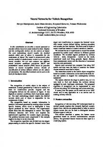
Fig. 1 presents the general scheme of integration of many classifiers into one ensemble system [7]
Fig. 1: The general scheme of classification using many classifiers
The measured signals of the process form the vector xin, subject to the preprocessing in the preprocessing blocks Pi (i=1, 2,…, M). The preprocessors may be of various kinds, stressing different aspects of signal. The features generated by the preprocessors form the vectors xi applied to the neural classifiers Ci. These vectors may vary in many aspects, including even the size (the number of diagnostic features). Each classifier has N outputs (N classes) and the output signals of each classifier are arranged in the form of vectors yi for i=1, 2, …, M, where M is the number of classification channels. These vectors are combined in the integrating unit to form one final output vector z of the classifier ( z ⊂ R N ). The highest value of elements of z indicates the membership to the appropriate class.
The integration of many classifiers into one ensemble of networks may be done using different methodologies. We will apply here four different approaches. They include: the simple majority voting, the weighted voting, KullbackLeibler divergence method and the modified Bayes combination. 2.1. The majority voting Suppose we have M neural network classifiers, which were trained on the same data. The committee of these classifiers assigns the pattern to the class that obtains the majority of the votes. Each classifier has the same influence on the final score. The majority voting is effective when the probability pr for each classifier to give the correct class label is equal for all input vectors xi and at the same time the classifier outputs are independent. However even in this case we can expect improvement over the individual accuracy pr only when pr is higher than 0.5 [6]. In the other case the majority voting integration does not bring any improvement over the individual classifier results. 2.2 The weighted voting If the classifiers in the ensemble system are not of the same accuracy then it is reasonable to give more competent classifiers more power for the final decision. The weighted majority voting combines the results of M classifiers with the weights according to the accuracy of each classifier obtained for the learning data. This is done through the integrating matrix W to form one response of the classifying system [11]. Let us denote by yi the vector of the classification results of ith classifier and by z the output vector of the ensemble system. The number of learning data pairs is denoted by p. The result of integration of all classifiers at the presentation of one particular input vector xin can be expressed now by the relation (1) z = Wy
[
]
T T M
N × NM
where y = y , y ,..., y and W ⊂ R . The position of the highest value element of z indicates the membership to the appropriate class. In adjusting the values of elements of the weight matrix W we have applied the minimization of the sum of squared error of the whole ensemble of the classifiers, measured on the learning data set [11]. This minimization leads to the solution expressed through the Moore-Penrose pseudoinverse in the form W = DY + , where Y is the NM × p matrix composed of p vectors y corresponding to p results of individual M classifications for learning data and D is the appropriate N × p matrix formed by the destination vectors associated with each learning pair of data. T 1
T 2
2.3 Kullback-Leibler divergence method Kullback-Leibler divergence measures the distance between the prior distribution and a posterior distribution. It is interpreted as the amount of information needed to change the prior probability distribution into the posterior one. In Kullback-Leibler divergence method [6] we calculate the ensemble probability µj supporting the jth class
given the actual input vector xin, as the normalized arithmetic mean 1 M µ j = ∑ d ij (2) M i =1 where dij means the probability of indicating jth class by ith classifier for the data of this class. This probability is determined in the testing mode for each multiple output classifier on the basis of the signal values on each output. In the case of one output classifier (for example SVM) we apply the one against one approach and the probability of each class is equal to the ratio of the number of victories of jth class to all possible indications. Observe that at two classes and 0-1 membership value to the particular class the Kullback-Leibler method is equivalent to the simple majority voting. 2.4 The modified naive Bayes combination This method assumes that the classifiers are mutually independent given a class label. We apply here the modification of the naive Bayes combination [6] since it gives more reliable results at zero estimated probability of any classifier. According to this modification the ensemble probability µj supporting the jth class is determined on the basis of the known results of testing the networks on the learning data and is given in the form (i ) M cm js + 1/ N i (3) µj = ∏ i =1 nj +1 where nj is the number of elements in training set for class j and cm (ijs)i is the element of the confusion matrix generated for learning data of ith classifier. The (j,s)th entry of the confusion matrix is the number of elements of the data set whose true class label was j and were assigned by ith classifier to sth class. 3.
THE NEURAL CLASSIFIERS
Different classifier solutions can be applied in practice. In this paper we will consider only the neural classifiers of different types. The considered classifiers include: the neuro-fuzzy networks of the modified Takagi-Sugeno-Kang (TSK) structure, the hybrid network and Support Vector Machine (SVM). 3.1 Hybrid fuzzy network The hybrid fuzzy network [10] is the combination of the fuzzy self-organizing layer and the multilayer perceptron (MLP) connected in cascade (generalization of the so called Hecht-Nielsen counter-propagation network). The fuzzy self-organizing layer is responsible for the fuzzy clusterization of the input data, in which the vector x is preclassified to all clusters with different membership grades. The particular membership value of some data vector xj to the cluster of the center ci is defined by the equation
uij (x j ) =
1
∑k =1 (d ij / d kj ) c
(4)
where c is the number of clusters and d ij = x j − c i . The position of the center of each cluster is adjusted in the learning procedure over all learning vectors xj. In our work we have applied the c-means algorithm [5]. The signals of the self-organizing neurons (the membership grades) form the input vector to the second subnetwork of MLP. MLP consists of many simple neuronlike processing units of sigmoidal activation function, grouped together in layers. Information is processed locally in each unit by computing the dot product between the corresponding input vector and the weight vector of the neuron. Traditionally training the network to produce a desired output vector when presented with an input vector involves systematically changing the weights of all neurons until the network produces the desired output within a given tolerance (error). The MLP part of the hybrid network is responsible for the association of the input vector with the appropriate class (the final classification). It is trained after the first selforganizing layer has been established. The training algorithm is identical to that used in training MLP alone [2]. 3.2 TSK neuro-fuzzy network Another neuro-fuzzy network involved in comparison is the modified Takagi-Sugeno-Kang (TSK) network [12]. It is implemented in the neuro-like structure realizing the fuzzy inference rules with the crisp TSK conclusion, described by the linear function. The TSK network can be associated with the approximation function y(x) K N y ( x j ) = ∑ µij (x j ) pi 0 + ∑ pik x k (5) i =1 k =1 where µij(x) is described by (4) and pik are the coefficients of the linear TSK functions f i (x ) = pi 0 + ∑k =1 pik x k . N
The parameters of the premise part of the inference rules (the membership values µij(xj)) are selected very precisely using Gustafson-Kessel self-organization algorithm [12]. After then they are frozen and don’t take part in further adaptation. It means that at application of the input vector xj (j = 1, 2, ..., p) to the network, the membership values µij(xj) are constant. The remaining parameters pij of the linear TSK functions can be then easily obtained by solving the set of linear equations following from equating the actual values of y(xj) and the destination values dj for j=1, 2, ..., p. The determination of these variables can be done in one step by using the singular value decomposition (SVD) algorithm and the pseudo-inverse technique. 3.3 SVM classifier The last classifier involved in the ensemble is the Support Vector Machine network [13,14]. It is known as the efficient tool for the classification problems, of a very good generalization ability. The SVM is a linear machine working in the high dimensional feature space formed by the nonlinear mapping of the n-dimensional input vector x into a K-dimensional feature space (K>n) through the use of the nonlinear function ϕ (x) . The equation of the
hyperplane separating two classes is defined in terms of K
these functions y ( x ) = ∑ w jϕ j (x ) + b = 0 , where b is the j =1
bias, and wj the synaptic weight of the network. The parameters of this separating hyperplane are adjusted in a way to maximize the distance between the closest representatives of both classes. In practice the learning problem of SVM is solved in two stages involving the solution of the primary and dual problems [13,14]. The most distinctive fact about SVM is that the learning task is simplified to the quadratic programming by introducing the Lagrange multipliers α i . All operations in learning and testing modes are done in SVM using kernel functions K ( x, x i ) , satisfying the Mercer conditions [13,14]. The most known kernels are Gaussian, polynomial, linear or spline functions. The output signal y(x) of the SVM network is finally determined as p
y ( x ) = ∑ αi d i K ( x i , x ) + b
(6)
i =1
where d i = ±1 is the binary destination value associated with the input vector xi. The positive value of the output signal means membership of the vector x to the particular class, while the negative one – to the opposite one. Although the SVM separates the data into two classes only, the recognition of more classes is straightforward by applying either one against one or one against all methods [3]. The more powerful is one against one approach, in which many SVM networks are trained to recognize between all combinations of two classes of data. For N classes we have to train N(N-1)/2 individual SVM networks. In the retrieval mode the vector x belongs to the class of the highest number of winnings in all combinations of classes. 4.
PREPROCESSING OF THE ECG SIGNALS
The important step in building the efficient classifier system is the generation of the diagnostic features, on the basis of which the classifier will recognize the pattern. In our approach to the problem we have applied two preprocessing methods of the data. One applies the Hermite representation of the QRS complex of the ECG and the second characterizes the QRS complex by the cumulants. 4.1 Hermite representation of theECG In Hermite basis function expansion method we represent the QRS complex by the series of Hermite functions [7]. Denote the QRS complex of the ECG curve by x(t). Its expansion into Hermite series may be written in the way
x(t ) =
N −1
∑ cnφn (t,σ )
(7)
n =0
where cn are the expansion coefficients, φn (t , σ ) - the Hermite basis functions of nth order and σ is the width parameter. The coefficients cn of Hermite basis functions expansion may be treated as the features used in the recognition
process. They may be obtained by minimizing the sum
[
N −1
squared error, E = ∑i x (ti ) − ∑n =0 cnφn (ti ,σ )
]
2
. This error
function represents the set of linear equations with respect to the coefficients cn. They can be easily solved by using singular value decomposition. In numerical calculations, we have presented the QRS segment of the ECG signal by 91 data points around the R peak (45 points before and 45 ones after). At the data sample rate 360 Hz, this gives a window of 250 ms, which is long enough to cover most of QRS signals. The data has been also additionally expanded by adding 45 zeros to each end of the QRS segment. The extra zeros are added to enforce that the beats are closed to zero outside the QRS complex. The width σ was chosen proportional to the width of the QRS complex. The modified QRS complexes have been decomposed onto a linear combination of 15 Hermite basis functions. These coefficients together with 2 classical features: the instantaneous RR interval of the beat (the time span between two consecutive R points) and the average RR interval of 10 preceding beats, form the 17-element feature vector x applied to the input of the classifier. 4.2 HOS characterization of the ECG Another approach to the feature generation is the application of the statistical description of the QRS curves. Three types of statistics have been applied: the second-, third- and fourth-order cumulants [9]. Application of the cumulant characterization of QRS complexes reduces the relative spread of the ECG characteristics belonging to the same type of heart rhythm and in this way makes the classification easier. As the features used in the heart rhythm recognition we have applied the values of the cumulants of the 2nd, 3rd and 4th orders at five points distributed evenly within the QRS length (for the 3rd and 4th order cumulants the diagonal slices have been calculated). For 91-element vector representation of the QRS complex the cumulants corresponding to the time lags of 15, 30, 45, 60 and 75 have been chosen. Additionally we have added two temporal features: one corresponding to the instantaneous RR interval of the beat and the second representing the average RR interval of 10 preceding beats. In this way each beat has been represented here by the 17element feature vector, with the first 15 elements corresponding to the higher order statistics of QRS complex (the second, third and fourth order cumulants, each represented by 5 values) and the last two - the temporal features of the actual QRS signal. 5. THE NUMERICAL EXPERIMENTS
5.1 The data base The numerical experiments have been directed for the recognition of the heartbeat on the basis of the ECG waveform. The recognition of arrhythmia is proceeded on the basis of the QRS segments of the registered ECG waveforms of 7 patients. The data have been taken from the MIT BIH Arrhythmia Database [8]. The important
difficulty of the accurate recognition of the arrhythmia type is the large variability of the morphology of the EEG rhythms belonging to the same class [8]. Moreover the beats belonging to different classes are also morphologically alike to each other. Hence the confusion of different classes is very likely. In our numerical experiments we have considered six types of arrhythmia: left bundle branch block (L), right bundle branch block (R), atrial premature beat (A), ventricular premature beat (V), ventricular flutter wave (I), ventricular escape beat (E), and the waveforms corresponding to the normal sinus rhythm (N). All these 7 rhythms have been discovered at one patient. So this kind of experiment may be regarded as the individual classifier specialized for the single patient. 3500 data pairs have been generated for the purpose of learning and 3068 were used for testing purposes. Table 1 presents the number of representative of the beat types used in testing only. Table 1 The number of testing samples of each beat type
Beat type
N
L
R
A
V
I
E
No
935
561
485
398
451
201
37
The limited number of representatives of some beat types (for example E or I) is the result of the limitation of the MIT BIH database [8]. 5.2 The results of numerical experiments In solving the problem of arrhythmia recognition we have relied on two sets of features. One set is related to the higher order statistics (HOS) and the second to the Hermite basis function expansion (HER) of the QRS part of the ECG waveform. Three different classifiers have been applied: SVM, Hybrid and TSK. All of them have been trained separately on both sets of features (HOS and HER) and their results have been combined together. In this way the ensemble of 6 recognition systems have been created. The integration of the results of all classifiers has been done using four presented above methods. We will limit the presentation of the results to the testing mode only, the most important from the practical point of view. The results are given in the form of the relative classification error, calculated as the ratio of all misclassification cases to the number of samples used in testing. Table 2 presents the results of testing all individual classifiers and the ensemble system integrated according to different methodologies. All classifier networks have been first learned on the same learning data set and then tested on another testing data set, the same in all cases. The best results of single classifiers refer to the application of SVMHER methodology (Hermite expansion for generation of features and SVM network classifier) and Hybrid-HOS (HOS representation for generation of features and hybrid network classifier). The worst results have been obtained at the application of TSK-HER solution (TSK classifier in combination with Hermite preprocessing of data). The relative difference between the accuracy of the best and worse classifier is very large (more than 60%). In spite of
large difference of the quality of the individual recognition systems even the simple majority voting was able to improve results significantly. However the best results have been obtained at the application of the weighted majority voting. The best individual result of 1.96% of relative misclassification (SVM-HER) has been improved to 1.37% (over 30% of relative improvement) in this case. Observe that all integration methods have improved the final accuracy of recognition in comparison to the best individual classification system.
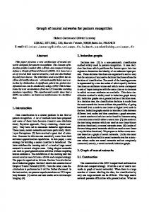
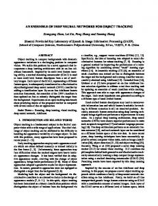
The notations used on the horizontal axis of the figure mean the type of the recognition system, for example H-HER means Hybrid-HER system, etc. It is seen that the relative improvement of the best integration scheme (weighted majority voting) with respect to the best individual classifier (SVM-HER) is over 30% and with respect to the worst one (TSK-HER)) almost 60%. The results prove that integrating the results of many classifiers of even not equal quality brings the significant improvement of the quality of performance of the whole classifier system.
Table 2 The average misclassification rate for the family of 7 beat types (the individual classifiers and ensemble of classifiers)
The quality of results can be assessed in details on the basis of the error distribution within different beat types. Table 3 presents the distribution of classification errors for the testing data in the form of the confusion matrix divided into different beat types. These results correspond to the best integration scheme. The diagonal entries of this matrix represent right recognition of the beat type and the off diagonal – the misclassifications. The column presents how the beats of particular type have been classified. The row indicates which beats have been classified as the type mentioned in this row. Thanks to the confusion matrix we can easily analyze which classes have been confused by our classifying system.
No
Classifier system
Testing error
1
Hybrid-HER (H-HER)
2.93%
2
Hybrid-HOS (H-HOS)
2.35%
3
TSK-HER (T-HER)
3.26%
4
TSK-HOS (T-HOS)
2.71%
5
SVM-HER (S-HER)
1.96%
6
SVM-HOS (S-HOS)
2.80%
7
Majority voting (MV)
1.63%
8
Weighted voting (WV)
1.37%
9
Kullback-Leibler (KL)
1.47%
10
Modified Bayes (MB)
1.56%
Generally we may state that integration of many classifiers improves the recognition results significantly. The improvement rate depends on the applied integration scheme and the quality of the individual classifiers. Fig. 2 presents the relative improvement of the final classification results of the ensemble obtained thanks to the applied integration method. Fig. 2a illustrates the improvement with regards to the best individual classifier (SVM-HER) and Fig. 2b to the worst one (TSK-HER).
Fig. 2 The relative improvement of different integration methods with respect to a) the best, b) the worst individual classifier
Table 3 The confusion matrix of the integrated classifying system for 7 types of rhythms of testing data
N L R A B I E
N 921 1 1 7 0 0 0
L 1 553 0 0 2 0 1
R 1 0 482 2 0 0 0
A 12 2 1 388 1 1 0
V 0 4 0 1 488 2 0
I 0 1 1 0 0 198 0
E 0 0 0 0 0 0 36
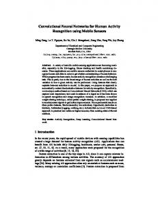
The analysis of the error distribution shows that some classes are confused more frequently than the others. It is evident that most misclassifications have been committed between two classes: N and A (12 N-rhythms have been classified as A-rhythms and 7 A-rhythms have been recognized as N-rhythms). This confusion is the result of large similarity of ECG waveforms for these two rhythms. The last but not least aspect of heart beat recognition is the analysis of how the abnormal rhythms have been separated from the normal one. In practice the most dangerous case is when the ill person is diagnosed as the healthy one (false negative diagnosed patient). To deal with such case we have introduced the quality measure equal to the number of all false negative diagnosed patients. Analyzing the obtained results we have noticed the evident improvement of this quality measure for the integration schemes, both in learning and in the testing mode. Table 4 presents the number of the false negative diagnoses for the individual classifiers and for all integrated systems under investigation. The results correspond to the testing data, not taking part in learning. The best results in terms of the number of the false negative diagnoses have been obtained for most of the integration methods (except KullbackLeibler approach). Fig. 3 presents the distribution of the
false negative cases for all proposed solutions (the individual classifiers and all integration schemes). Table 4 The comparison of the number of false negative diagnoses for different solution of the classifying systems
No
Classifier system
1
Hybrid-HER
No of false negative cases 22
2
Hybrid-HOS
10
3
TSK-HER
23
4
TSK-HOS
36
5
SVM-HER
14
6
SVM-HOS
11
7
Majority voting
9
8
Weighted voting KullbackLeibler Modified Bayes
9
9 10
11 9
The interesting is that most of the integration schemes have produced the same number of false negative diagnoses, much better than the average number obtained at application of individual classifiers. The Kullback-Leibler method has produced slightly worse results.
The experiments performed for seven heart beat types taken from MIT BIH AD have shown that integration of the results of many classifiers improves the quality of the final classification system. The improvement is observed in terms of the accuracy of recognition as well as of the number of false negative diagnoses. To the best integration approaches belong the weighted majority, modified Bayes and Kullback-Leibler methods. They have resulted in the reduction of not only the total classification errors and at the same time also in the reduction of the most dangerous false negative cases of diagnosis. The results presented in the paper confirm our conjecture that a highly reliable classifier can be obtained by combining a number of classifiers which exhibit an average performance. REFERENCES
[1]
[2] [3]
[4]
[5]
[6] [7]
[8] [9] [10]
[11]
[12] Fig. 3 The comparison of the number of the false negative cases corresponding to individual classifiers and to all ensemble systems
6. CONCLUSIONS
[13]
The paper has presented and compared different methods of integration of the results of many individual neural classifiers combined into one classification system. The applied classifiers include: hybrid neural network, neurofuzzy TSK network and support vector machine classifiers. The ensemble system applied majority and weighted voting, Kullback-Leibler divergence and modified Bayes methods.
[14]
P. de Chazal P., M. O'Dwyer, R. B. Reilly, Automatic classification of heartbeats using ECG morphology and heartbeat interval features, IEEE Trans. on Biomed. Eng, 2004, vol. 51 pp. 1196-1206 S. Haykin, Neural networks, comprehensive foundation, Prentice Hall, 1999, New Jersey C. W. Hsu, C. J. Lin, A comparison methods for multi class support vector machines, IEEE Trans. Neural Networks Vol. 13, pp. 415-425, 2002 Y. H. Hu, S. Palreddy, W. Tompkins, A patient adaptable ECG beat classifier using a mixture of experts approach, IEEE Trans. Biomed. Eng., 1997, vol. 44, pp. 891 – 900 L. Jang, C. T. Sun, E. Mizutani, Neuro-fuzzy and Soft Computing, Prentice Hall, New Jersey, 1997 L. Kuncheva, Combining pattern classifiers: methods and algorithms, Wiley, N. J., 2004 M. Lagerholm, C. Peterson, G. Braccini, L. Edenbrandt, L. Sornmo, Clustering ECG complexes using Hermite functions and self-organizing maps, IEEE Tr. Biomed. Eng., 2000, vol. 47, pp. 838-847 R. Mark, G. Moody, MIT-BIH arrhythmia database directory, MIT C. Nikias, A. Petropulu, Higher order spectral analysis, Prentice Hall, N. J., 1993 S. Osowski, Tran Hoai Linh, ECG beat recognition using fuzzy hybrid neural network, IEEE Trans. on Biomedical Engineering, vol. 48, pp. 1265-1271, 2001 S. Osowski, L. Tran Hoai, T. Markiewicz, Support Vector Machine based expert system for reliable heart beat recognition, IEEE Trans. on Biomedical Engineering, 2004, vol. 51 , pp. 582-589 S. Osowski, L. Tran Hoai, On-line heart beat recognition using Hermite polynomials and neurofuzzy network, IEEE Trans. on Instrum. and Measur., 2003, vol. 52, pp. 1224-1230 B. Schölkopf, A. Smola, Learning with Kernels, Cambridge MA, MIT Press, 2002 V. Vapnik, Statistical learning theory, Wiley, N.Y. 1998