Oct 6, 2006 - lution is ensures the QoS requirements of all the WiMAX service classes and shares fairly free resources achieving the work-conserving ...
Ensuring the QoS Requirements in 802.16 Scheduling Alexander Sayenko, Olli Alanen, Juha Karhula, Timo Ham ¨ al ¨ ainen ¨ Telecommunication laboratory, MIT department University of Jyvaskyl ¨ a, ¨ Finland {sayenko,opalanen,jkarhula,timoh}@cc.jyu.fi
ABSTRACT
The standard defines two basic operational modes: pointto-multipoint (PMP) and mesh. In the mesh mode, subscriber stations (SS) can communicate to each other and to the base stations (BS). In the PMP mode, the SSs are only allowed to communicate through the BS. It is anticipated that providers will use the PMP mode to connect customers to the Internet. In this case, the SSs do not send data one to each other and, at the same time, a provider can control the environment to ensure the QoS requirements of customers. An important principle of WiMAX is that it is connection oriented. It means that an SS must register to the base station before it can start to send or receive data. During the registration process, an SS can negotiate the initial QoS requirements with the BS. These requirements can be changed later, and a new connection may also be established on demand. The QoS requirements may be either per connection based (GPC) or per subscriber station based (GPSS). In this paper, we do not take in to account which one of these modes is used because in GPSS, it is the responsibility of an SS to collect its service requirements to one connection. The basic approach for providing the QoS guarantees in the WiMAX network is that the BS does the scheduling for both the uplink and downlink directions. In other words, an algorithm at the BS has to translate the QoS requirements of SSs into the appropriate number of slots. The algorithm can also account for the bandwidth request size that specifies size of the SS input buffer.1 When the BS makes a scheduling decision, it informs all SSs about it by using the UL-MAP and DL-MAP messages in the beginning of each frame. These special messages define explicitly slots that are allocated to each SS in both the uplink and downlink directions. The scheduling policy, i.e. an algorithm to allocate slots, is not defined in the WiMAX specification, but rather is open for alternative implementations. This paper presents a scheduling solution for the WiMAX base station. There are several articles on the WiMAX QoS scheduling that have presented architectures and scheduling disciplines to guarantee QoS. However, in [16, 6] authors have focused mainly on the scheduling issues and components of the QoS architecture without presenting any exact method with the extensive simulation results. Several research works [4, 17, 13] propose complex schedulers or
IEEE 802.16 standard defines the wireless broadband access network technology called WiMAX. WiMAX introduces several interesting advantages, and one of them is the support for QoS at the MAC level. For these purposes, the base station must allocate slots based on some algorithm. We propose a simple, yet efficient, solution for the WiMAX base station that is capable of allocating slots based on the QoS requirements, bandwidth request sizes, and the WiMAX network parameters. To test the proposed solution, we have implemented the WiMAX MAC layer in the NS-2 simulator. Several simulation scenarios are presented that demonstrate how the scheduling solution allocates resources in various cases. Simulation results reveal the proposed scheduling solution is ensures the QoS requirements of all the WiMAX service classes and shares fairly free resources achieving the work-conserving behaviour.
Categories and Subject Descriptors C.2.1 [Computer-Communication Networks]: Network Architecture and Design—Wireless communication
General Terms Algorithms
Keywords QoS, WiMAX, scheduling, NS-2
1.
INTRODUCTION
WiMAX is an IEEE standard for the wireless broadband access network [1]. The main advantages of WiMAX when compared to other access network technologies are the longer range and more sophisticated support for the Quality-ofService (QoS) at the MAC level. Several different types of applications and services can be used in the WiMAX networks and the MAC layer is designed to support this convergence.
Permission to make digital or hard copies of all or part of this work for personal or classroom use is granted without fee provided that copies are not made or distributed for profit or commercial advantage and that copies bear this notice and the full citation on the first page. To copy otherwise, to republish, to post on servers or to redistribute to lists, requires prior specific permission and/or a fee. MSWiM’06, October 2–6, 2006, Torremolinos, Malaga, Spain. Copyright 2006 ACM 1-59593-477-4/06/0010 ...$5.00.
1
These requests can be sent as either independent messages or piggy-packed with some other packets. Subscriber stations can also use special contention slots to send the bandwidth requests. However, collisions can occur. The algorithm for the contention period is an important issue, but it is out of the scope of this article. Some suggestions can be found in [8] and [5].
108
even an hierarchy of schedulers, such as Earliest Deadline First (EDF), Deficit Round Robin (DRR) [15], Weighted Fair Queueing (WFQ) [14], and Worst-case Weighted Fair Queueing (W2 FQ) [3]. However, it is a challenging task to use an hierarchy of schedulers because the per-connection QoS requirements should be translated into the scheduler configuration at each level. Furthermore, it is not enough to calculate the scheduler configuration only once when an SS joins or leaves the network. As SSs send data, their request sizes change all the time. As a result, the scheduler at the BS should reassign slots. For exactly these reasons we suggest to use one level with a simple scheduling mechanism that is based conceptually on the round-robin (RR) approach. A simpler solution is better, because there is not much time to do the scheduling decision. For instance, one of the possible configuration values is 400 frames per second [1]. Thus, the BS should make 400 scheduling decision per one second to achieve the accurate and fair resource allocation. When compared to the previous research works, our solution supports all the WiMAX service classes. We propose to allocate slots based on the QoS requirements and bandwidth request sizes. Furthermore, for each service class we propose a policy to allocate slots so that the BS can perform polling. The previous research works on the scheduling in WiMAX are based on simulations that were run in simple environments, such as MATLAB. We have tested our scheduling algorithm in the NS-2 simulator that offers a significantly better possibility to simulate realistic network topologies, traffic characteristics, and behaviour of the transport protocols, such as TCP. For these purposes, we have implemented the WiMAX MAC and PHY layers. The rest of the article is organized as follows. Section 2 presents the theory behind our scheduling proposal. This section presents calculations on how to convert the QoS requirements into the number of slots, how to allocate free slots, how to order slots, and how to estimate the WiMAX MAC overhead. Next, Section 3 describes the simulation environment that is used to test the proposed scheduler. Several simulation scenarios are presented and the simulation results are analysed. Finally, Section 4 concludes the article and presents the further directions of our work.
2.
At the same time, there are differences between the WRR scheduler and the WiMAX environment. The most important one is that WRR behaves work-conservingly skipping empty queues and starting to serve the next queue when all packets from the current one are sent. Since the WiMAX frame is fixed, it behaves non-work-conservingly. In other words, if there are slots that are not allocated to any connection, then some bandwidth resources will be wasted. Another important difference between WRR and WiMAX is that in WRR we can specify the number of packets to send from each queue during a round, but we cannot influence the order. In WiMAX, there is a possibility to assign explicitly each slot to some connection, thus specifying the serving order. Though it makes scheduling in WiMAX more complicated, it allows to control the maximum delay and jitter values. Based on the presented above considerations, we anticipate that the WiMAX scheduling should comprise three major stages: 1. Allocation of the minimum number of slots. At this stage, the task of the BS is to calculate the minimum number of slots for each connection to ensure the basic QoS requirements. 2. Allocation of unused slots. At this stage, the BS has to assign free slots to some connections to avoid non-work-conserving behaviour. 3. Order of slots. At this stage, the BS has to select the order of slots to improve the provisioning of the QoS guarantees. It is worth mentioning that only the first stage is mandatory. The WiMAX network still will schedule slots from SSs if the BS does not implement the second and the third stage. However, we anticipate that also the second stage must be mandatory. Though there are reasons to use and not to use the non-work-conserving behaviour [18], we expect that the WiMAX providers will use the usage-based pricing, as many other wireless providers do. Thus, it is not likely that a provider would agree on wasting bandwidth resources if there are users willing to send data and pay for it. Even if the time-based pricing is used, i.e. month fee, then a provider is still interested in achieving the work-conserving behaviour because it will result in better service. The scheduling solution we propose concerns only the scheduler at the BS that allocates resources in the WiMAX network. Each SS is free to choose the scheduling discipline at its WiMAX output interface because it will control how the resources, which are allocated by the BS, will be shared between local applications and/or sub-connections in the GPSS mode. For instance, if an SS is a router that connects LAN to the Internet through the WiMAX network, then the router may control how resources are shared between the local workstations or subdepartments. In the same way, the designers of the WiMAX BS are free to choose the scheduling discipline at the interface that connects the BS to the wired medium. However, we anticipate that the BS should be connected to the wired medium with a link, whose bandwidth is larger than the theoretical maximum bandwidth of the WiMAX network. Thus, simple First-Come-FirstServed will suffice. The subsequent subsections present the description for the scheduling stages that we mentioned above.
OUR SCHEDULING PROPOSAL
The proposed scheduling discipline for the WiMAX BS is conceptually similar to the Weighted Round Robin (WRR) scheduler [12]. Indeed, each connection can be treated as a separate session, while the number of slots, which the BS has to allocate for each connection based on its QoS requirements, is the weight value of the WRR scheduler. Since all slots are of the same size, there is no need to use other complex scheduling disciplines, such as fair queuing (FQ) [7]. Indeed, FQ was proposed to achieve fair resource allocation in the Internet, in which packet sizes vary. Furthermore, the usage of FQ will even complicate the scheduling process. The reason is that weight values of the FQ schedulers are the floating-point numbers, while the WiMAX BS has to allocate some number of slots, which is the integer value. If one uses FQ, then an additional step will always be necessary to convert the FQ floating-point weight values into the integer number of slots. Thus, it is more efficient to calculate the number of slots as integer values bypassing unnecessary intermediate steps. Similar considerations apply for the more sophisticated RR disciplines, such as DRR [15], that aim to emulate FQ.
109
2.1 Allocating the minimum number of slots
� Ri = 0, � 1, � Nimin = Bimin � , Ri > 0,
Suppose Bi is the bandwidth requirement of the ith connection. Also, suppose that Si stands for the slot size, i.e. the number of bytes a connection can send in one slot. It is worth noting that the slot size Si depends on an SS since the latter can use different modulations to transmit data. Based on the introduced above parameters, one can calculate the number of slots within each frame by using the following expression: Ni =
� Nimax = min
�� ,
(4)
• As mentioned above, the purpose of the ertPS class is to combine efficiency of the UGS and rtPS classes. The typical application that will use this class is VoIP with the silence suppression. If the speech is active, then a codec outputs data at some constant rate. From this point of view, resource allocation is quite similar to UGS. At the same time, ertPS is allowed to send the bandwidth requests. Since the request size equals zero during a silence period, the BS can allocate one slot thus enabling an SS to ask for more bandwidth when the active phase of the speech starts. From this point of view, the allocation of slots is similar to the rtPS class:
(1)
Nimin
=
Nimax
� Ri = 0, (5a) � 1, � = Bi � , Ri > 0, (5b) Si FPS
∀i | Ci = ertPS. It is interesting to note that according to [2], the ertPS connection can also send the bandwidth requests during the contention period. Thus, if the request size equals zero, then the BS may avoid reserving one slot thus achieving better resource allocation. However, it is understandable that the ertPS connection may experience longer delays or even packet drops before it can send the bandwidth request during the contention period. We address this tradeoff problem to our future studies.
• Unlike other service classes, the UGS class does not send the bandwidth requests and cannot participate in the contention. Thus, we always have to allocate the necessary number of slots based on the bandwidth requirement (the UGS class does not have minimum/ maximum bandwidth requirements):
• The logic behind allocating slots for the nrtPS class is quite similar to the rtPS class. The only difference is that if the request size equals zero, then we do not allocate any slots at all. Unlike the rtPS class, nrtPS connections can participate in the contention. By not allocating slots when the request size equals zero, we preserve some slots that later can be allotted for those nodes that really need them. Another important difference is that we also analyse the value of the request size while calculating the minimum number of slots. If it is smaller than the number of slots a connection needs to send data at the minimum sustained rate, then we just allocate the number of slots that is necessary to send the amount of data specified in the bandwidth request. By this we can achieve more optimal allocation of slots in those cases when a connection sends data at a rate lower than the minimum one. It can be the case for some TCP-based applications, such as Web browsers.
�
Bi , Si FPS
�
Bimax Ri , Si FPS Si
∀i | Ci = rtPS.
where FPS stands for the number of frames the WiMAX BS sends per one second. The idea behind (1) is that we determine the overall number of slots necessary to ensure the bandwidth requirements, and then divide it by the number of frames to calculate the number of slots we have to allocate in one frame. In practice, to calculate the number of slots for the WiMAX connections we also have to take their types, or classes, and the request sizes into account. There are four distinct service classes defined by the 802.16d specification: Unsolicited Grant Service (UGS), real-time Polling Service (rtPS), nonreal-time Polling Service (nrtPS) and Best Effort (BE). UGS is designated for fixed-size data with periodic intervals. The rtPS class is similar to UGS but for variable-rate traffic, such as MPEG video data. The nrtPS class is designed for applications that are not sensitive to delay and jitter. The 802.16e specification [2] has added another class, extended real-time Polling Service (ertPS). The purpose of this class is to combine efficiency of the UGS and rtPS classes. The difference between the UGS class is that whereas UGS allocations are fixed, ertPS allocations are dynamic. Suppose that Bimin and Bimax are the minimum and maximum bandwidth requirements. Also, suppose that Ci stands for the ith connection class and Ri stands for the request size. Then, depending on the service class the number of slots for each connection is calculated differently.
Nimin = Nimax =
(3b)
Si FPS
�
Bi , Si FPS
(3a)
(2)
∀i | Ci = UGS. • In the case of the rtPS class we allocate slots based on the bandwidth requirements and the request size Ri . If the request size equals zero, then we allocate one slot. We cannot allocate zero slots because the rtPS connection cannot participate in the contention. If a connection is allocated at least one slot, then it has a possibility to send the bandwidth request, thus asking BS to allocate more slots. If the request size is bigger than zero, then we calculate the minimum and maximum number of slots based on the minimum and maximum bandwidth requirements:
110
Suppose, A is a set with connections for which free slots should be assigned; all elements in A is sorted in such a max way that Ni−1 < Nimax . Then, by applying the following expressions for each connection i ∈ A it is possible allocate fairly free slots:
� 0, Ri = 0, (6a) � � min � �� min Ni = Bi Ri � min , ,Ri > 0,(6b) Si FPS
� Nimax = min
Si
�
Bimax Ri , Si FPS Si
�� ,
�
Niadd = min Nimax − Nimin ,
(6c)
∀i | Ci = nrtPS. • Since the BE class does not have any requirements at all, we do not reserve any slots for the connections that belong to this class. However, the maximum number of slots allocated for the BE connection should not exceed the amount of data specified in the bandwidth request: Nimin = 0,
(7a)
Ri , ∀i | Ci = BE Si
(7b)
�
Nimax =
F
,
(9a)
Ni = N min + Niadd ,
(9b)
Niadd ,
(9c) (9d)
f ree
←F − remove i from A. f ree
2.3 Order of slots When the BS calculates the number of slots for every connection, it can specify an order of slots. The simplest solution is to put all the slots consecutively. However, a better approach is to interleave the slots to decrease the maximum jitter and delay values.
�
� SS1
�
SS2
SS2
SS3
SS3 max. jitter
-
SS2 max. jitter SS3
SS3
SS3
SS1–1 slot, SS2–2slots, SS3–4 slots
2.2 Allocating free slots
SS1
SS2
SS2
SS3
...
-
(a) non-interleaved
If there are unused slots, it makes sense to allocate them to other connections. The reason is that the frame has the fixed size. As explained earlier, if we do not allocate unused slots to some connections, then the WiMAX BS will have the non-work-conserving behaviour. Having analysed the service classes, it is possible to arrive at the conclusion that it makes sense to allocate unused slots to the rtPS, nrtPS, and BE connections. There is no need to allocate slots to the UGS or ertPS connections since it is not likely that the constant-rate applications will increase their transmission rates. First, we determine the number of free slots that remains after we ensure the minimum bandwidth guarantees.
�
Nimin ,
� SS1
�
SS2
SS3
SS3
SS2
� SS3 max.jit. SS2 max. jitter -
SS3
SS1–1 slot, SS2–2slots, SS3–4 slots
SS3
SS1
SS2
SS3
SS3
...
-
(b) interleaved Figure 1: Non-interleaved and interleaved slot order Suppose, there are three SSs; the first SS is assigned one slots, the second one is assigned two slots, and the third one is assigned four slots. Then, Fig. 1(a) presents the noninterleaved order of slots when the scheduler at the BS places all the slots consecutively. The figure also presents the maximum distance, i.e. jitter, between two slots belonging to SS2 and SS3. Fig. 1(b) presents the slot order, in which slots belonging to different SSs are interleaved. As follows, from this figure, the maximum jitter for SS2 and SS3 decreases.
(8)
i
where F is the size for the uplink or downlink part of the WiMAX frame. If F f ree = 0, then there are no free slots at all. Furthermore, if F f ree < 0 then there are not enough slots even to ensure the minimum bandwidth requirements. By this the previous stage can be used implicitly as a simple admission control module.2 2
�
Depending on the class of connections kept in A, slightly different resource allocation can be achieved. At one extreme point, A may contain connections of the rtPS, nrtPS, and BE classes. At another extreme point, A may contain connections belonging to one specific class. In other words, first free slots are allocated for the rtPS connections, then for the nrtPS connections, and finally for the BE connections. The implementation we have at the moment first allocates free slots for the rtPS and nrtPS connection, and then what remains is distributed between the BE connections.
Expressions (2)-(6c) can be applied both to the uplink and downlink directions. By this we can calculate the minimum and maximum number of slots for the uplink and downlink parts of the frame. The only difference is that while calculating the number of slots for the downlink part, we can take the queue size into account instead of the request size. The size of a queue has the same physical sense as the request size. For these purposes, the BS can allocate a separate queue for each active connection in the downlink direction. It is necessary because the BS should have a possibility to fetch independently packets for each connection based on the number of slots assigned by the scheduler. Furthermore, a separate queue simplifies the process of tracking the queue size.
F f ree = F −
F f ree |A|
for the ranging and contention slots. Also, the variable size of the UL-MAP, DL-MAP, UCD, and DCD messages creates additional challenges for the designers of the WiMAX admission control model. A simple admission control model is presented in [11].
A full featured admission control model should also account
111
In this paper, we do not propose a universal implementation for the interleaving algorithm, neither do we try to estimate the worst-case jitter based on the number of SSs and allocated slots. Our intention is to present that interleaving, even in its simplest form, can improve the delay characteristics. We anticipate that interleaving should be always done for the UGS, ertPS, and possible rtPS connections even if they do not have explicit delay requirements. Here, we present a sample algorithm we use at the moment. In the first step, the algorithm calculates the ideal distance between slots for every connection. Then, based on these distances, the algorithm takes all the connections one by one and tries to assign slots to the proper positions. The algorithm starts to place slots for the UGS connections and then for the ertPS and rtPS connections. If the chosen slot is already assigned to another connection, then the closest free slot is chosen. The remaining slots can just be filled with the slots for the nrtPS and BE connections because they do not have any delay or jitter requirements. By this we can make this stage a little bit faster. The only disadvantage of the interleaving process is the increased size of the UL-MAP and DL-MAP messages. Indeed, by allocating slots in several bursts, the size of the ULMAP or DL-MAP messages increases resulting in a fewer number of slots available for user data.
whether the packing is used or not, each packet and the packet fragment may be appended with the optional CRC field that occupies 32 bits. Hence, we will use the following notation: H M is the size of the MAC header, H F is the size of the fragmentation subheader, H P is the size of the packing subheader, H C is the CRC field, and Pi is the SDU size of the ith connection. To clarify calculations, two subcases will be considered that depend on the SDU size announced by a connection. • If SDU with all the MAC headers is less than a slot size, then usually a slot contains a tail part of a previous SDU followed by zero or more full SDUs and then a head part of the next SDU. If the BS does not use packing, then the MAC header is added to the beginning of a full SDU or its fragment. There is also the fragmentation subheader in the case of the SDU fragment. Fig. 2(a) presents the graphical interpretation for this case (for the sake of clarity, �the optional CRC field is omitted). Thus, if Pi ≤ Si − H M + H C , then
�
+ H +H
2.4 Calculating the overhead
M
C
� Si −2(H M +H F +H C ) �
(11)
.
Pi +H M +H C
• If SDU with the MAC headers does not fit into a slot, then the usual arrangement of a slot contains a tail part of the previous SDU and a head part of the next SDU. As in the considered above case, each packet fragment is preceded with the MAC header and the fragmentation subheader. Fig. 2(b) presents the � graphical interpretation. Thus, if Pi > Si − H M + H C , then
�
Bi , � Si FPS
�
The idea behind (11) is that we account for the overhead caused by two SDU fragments (in the beginning and the end of a slot) and zero or more full SDUs.
It is important to note that the basic expression (1) does not take the WiMAX MAC header overhead into account. Each slot has the mandatory MAC header and may have other subheaders (fragmentation or packing) and the optional CRC filed. Thus, the number of bytes available for user data is less when compared to the overall slot size. Based on this it is possible to modify (1) as follows: Ni =
�
�
Si = Si − 2 H M +H F +H C +
(10)
�
�
Si = Si − 2 H M + H F + H C
�
where Si stands for the number of bytes available for user data. In the similar way one can modify (2)-(6c). The cal� culations for Si will depend on the service data unit (SDU) size and other parameters, such as whether the data unit is constant or not, wether the packing is enabled or not, etc. We anticipate that the overhead should be calculated only for the UGS and ertPS connections, and in some cases for the rtPS connections. As we will present later, the overhead estimation depends on the SDU size announced by an SS. However, it is likely that the SDU size may vary significantly for the nrtPS and BE connections. Furthermore, most nrtPS and BE connections will correspond to the TCP-based applications that always wait for the positive acknowledgements. As opposed to this, the UGS and ertPS connections usually transmit data at some constant rate. Thus, if we do not estimate the overhead for such a connection then it will experience constant packet drops. Depending on whether the BS supports packing or not, two cases will be considered. If the BS does not use packing, then every packet and the packet fragment is preceded with the MAC header. In the case of the packet fragment, the fragmentation subheader is also added. If the BS uses packing, then the MAC header appears only in the beginning of a slot, and each packet fragment is preceded with the packing subheader. Furthermore, regardless of the fact
�
(12)
In (12), we account for the overhead caused by the MAC header and the fragmentation subheader that precede every SDU fragment. HM
HF
frag
HM
HM
full
�
(a) Pi ≤ Si − H M + H C HM
HF
frag
HM
HF
frag
HF
frag
�
(b) Pi > Si − H M + H C
Figure 2: Overhead when packing is not used It is worth noting that �(12) is just a particular case of (11). Indeed, if Pi > Si − H M + H C , then
Si −2(H M +H F +H C ) Pi +H M +H C
= 0,
and (11) yields (12). Thus, (11) is the basic formula for calculating the overhead when the packing is not used.
112
BE connections. Though WiMAX supports several service classes, we anticipate that the major number of connections will use the BE class. Thus, it is important to ensure that the available bandwidth resources are shared fairly between the active BE connections regardless of their number. Besides, the purpose of this scenario is to ensure that if there are free slots, then they will be allotted to the BE connections to achieve the work-conserving behaviour. The second scenario will present the multi-service case, in which a provider has to support connections with different WiMAX classes and traffic characteristics. The purpose of this scenario is to ensure that the scheduler at the BS takes the service class into account and allocates slots based on the QoS requirements and the request sizes sent by SSs. Another purpose is to test that the scheduler at the BS takes the MAC overhead into account. The third scenario presents a case with several UGS connections that use different modulations and change them in the course of time. The purpose of this scenario is to ensure that the proposed scheduling solution allocates the sufficient number of slots by taking the slot size and the MAC overhead into account. It is also important to test that the scheduler allocates resources accurately in accordance with the QoS requirements and the slot size. Each simulation scenario includes a wired node, to which all the wireless SSs send data. The wired node is connected to the BS with a link, whose bandwidth and delay are 1,000,000,000 bps and 2 ms, respectively. We set the bandwidth of this link to be larger than the bandwidth of the WiMAX network so that the latter is the bottleneck part of the network structure. By this we can test that the scheduler at the BS allocates sufficient number of slots for all SSs in accordance with their QoS requirements. Regardless of the simulation scenario, the general parameters of the WiMAX network are the same. There is one BS that controls the traffic of the WiMAX network. The parameters of the BS are 400 frames per second, and 80 slots per one frame. Duration of one time slot corresponds to the 7 MHz frequency band. The physical layer is OFDM. The amount of data an SS can send within one slot depends on the chosen modulation. Since we use different modulations in the simulation scenarios, we will mention explicitly the modulation for each SS. Both the BS and all SSs use the packing in all simulation scenarios. Neither the BS nor SSs use the CRC field while sending packets. It should be noted that the BS reserves certain number of slots for the contention and the ranging periods. The length of the contention period for the nrtPS and BE connections is always one slot (since there are not so much SSs in the simulation scenarios, one slot will suffice). However, the scheduler at the BS reserves this slot only if there are nrtPS or BE connections that have not been allocated any slot at all. Otherwise, having at least one slot, each connection can always send bandwidth requests. As a result, there is no sense in allocating slots for the contention period. At the same time, the BS always allocates one slot for the ranging period because an SS can join the network at any time.
If the BS and SSs support packing, then the formulas are quite similar to the ones presented above. The only difference is that the MAC header appears only once in the beginning of each slot and the packing subheader is used instead of the fragmentation subheader:
�
�
�
Si = Si − H M +2 H P +H C +
�
+ H +H P
C
� � Si − �H M +2(H P +H C ) ��
(13)
.
Pi +H P +H C
Fig. 3 presents the graphical interpretation of (13) for small and large SDUs. HM
HP
frag
HP
full
�
(a) Pi ≤ Si − H M + H HM
HP
frag
HP
HP
�
(b) Pi > Si − H M + H
frag
C frag
C
Figure 3: Overhead when packing is used Regardless of the fact whether the packing is on or off, if the BS does not use the CRC field, then it is enough set H C to zero to avoid overestimating the overhead.
3.
SIMULATION
3.1 Environment This section presents the simulation results for the proposed scheduling solution. To test it, we have implemented the WiMAX MAC layer and the scheduling mechanism in the NS-2 simulator. The MAC implementation contains the main features of the WiMAX standard, such as downlink and uplink transmission, packing, fragmentation, the contention and ranging periods. We have also implemented the most important MAC signaling messages, such as UL-MAP and DL-MAP, UCD and DCD, ranging (RNG), registration (REG), dynamic service addition (DSA), and dynamic service change (DSC). The implementation also supports the OFDM physical layer. However, since we are interested in the scheduling that is done on the MAC level, we do not simulate errors at the physical layer. Current implementation also supports different modulations. Table 1 presents slot size for different modulations and channel coding types. Table 1: Slot sizes for the OFDM PHY Modulation Channel coding Slot size (B) 64-QAM 3/4 108 64-QAM 2/3 96 16-QAM 3/4 72 16-QAM 1/2 48 QPSK 3/4 36 QPSK 1/2 24
3.2 Simulation scenario 1 Fig. 4 presents the network structure for the first simulation scenario. The network includes one BS and fifteen SSs that use the BE connection. All the SSs use the same modulation, 64-QAM 3/4. The purpose of this scenario is
We present several simulation scenarios to study thoroughly the proposed scheduling solution. In the first scenario, we study how the bandwidth is allocated between the
113
2.5e+07
to ensure that the scheduler at the BS allocates resources fairly between the BE connections regardless of their number and regardless of the fact that they do not have any QoS requirements.
SS1(BE) SS2(BE) SS3(BE) SS4(BE) SS5(BE) SS6(BE) SS7(BE) SS8(BE) SS9(BE) SS10(BE) SS11(BE) SS12(BE) SS13(BE) SS14(BE) SS15(BE) TOTAL
Throughput, B (bps)
2e+07
destination node 1,000,000,000 bps 2 ms 15 stations
BE
1.5e+07
1e+07
5e+06
400 frames per second 80 slots per frame 0 0
2
4
6
Figure 4: Network structure
8
10 Time, t (s)
12
14
16
18
20
Figure 5: Throughput
Each SS establishes one uplink and downlink connection to the BS. An SS hosts exactly one FTP application that sends data over the TCP protocol to the wired node. The TCP protocol waits for the positive acknowledgements and adjusts its transmission rate according to the available resources. Thus, the adaptive behaviour of the TCP protocol is a good way to test how the scheduler at BS allocates resources and to study the behaviour of TCP over WiMAX.
connection receives more slots when compared to the situation when there are many active applications. Fig. 5 also presents the total bandwidth observed at the BS output interface. The reason it declines when the number of active applications increases is the fact that the UL-MAP and DLMAP messages become bigger thus leaving less slots for the user data. Small fluctuations are explained by the fact the BS has to allocate sometimes a slot for the contention period.
Table 2: Active applications Simulation time SS 0–5 5–10 10–15 15–20 √ √ √ SS1 – SS3 √ √ SS4 – SS5 √ SS6 – SS13 √ √ SS14 – SS15
3.3 Simulation scenario 2 Fig. 6 presents the network structure for the second simulation scenario. The network comprises one WiMAX BS and seven SSs. There is one UGS connection, one ertPS connection, two rtPS and nrtPS connections, and also one BE connection. All the SSs use the 64-QAM 3/4 modulation.
To study the resource allocation with different number of active flows, we will turn on/off some of the FTP applications. If there are only a few active applications, then the scheduler at the BS should allocate more slots for the active ones, which in turn should increase their transmission rates. Consequently, if there are many active applications, then the scheduler at the BS will try to allocate resources equally between them. As a result, each connection will be allotted only a few slots. Table 2 presents information about which applications are active at different moment of times. In the beginning, there are only three active applications, then their number is five, then all the applications are active, and finally only two applications transmit data. It is worth mentioning that the scheduler allocates slots for the BE connections based on their request sizes, not based on the fact that an SS has joined the network. For these purposes, all the SSs enter the network in the beginning of a simulation run. Thus, during a simulation all the fifteen WiMAX connections are active, while the number of active applications vary. Fig. 5 presents the throughput for each SS. Data was gathered at the output interface of the BS connected to the wired medium. The figure also presents the uplink throughput that is measured as the total throughput of data that leaves the BS wired interface. As follows from the results, the scheduler at the BS always allocates resources fairly between the active BE connections. As the request sizes change, the scheduler recalculates the number of slots for each connection. If there are only a few active applications, then each
SS2
SS1
SS3 UGS ertPS
rtPS
destination node
SS4
1,000,000,000 bps 2 ms rtPS
SS5
nrtPS
400 frames per second 80 slots per frame
SS6 SS7 nrtPS BE
Figure 6: Network structure The purpose of this scenario is to test how the scheduler at the BS allocates resources between connections that belong to different services classes. For these purposes, applications at the SSs generate traffic patterns that correspond to different service types. Table 3 presents the QoS requirements of applications and traffic types they generate. As in the previous scenario, each SS hosts exactly one application and establishes one uplink connection to the BS. SS5 and SS6 also establish a down-
114
at the BS allocates sufficient number of slots by taking into account the QoS requirements and the MAC overhead. Since the ertPS connection corresponds to the VoIP data, its throughput is determined by the ON/OFF model that simulates the speech. During the active phase the ertPS connection throughput is 80,000 bps. Thus, the scheduler allocates sufficient slots for this connection. During the silence phase the throughput is zero. However, the scheduler allocates one slots so that this connection can send the bandwidth request as soon as possible when the active phase starts. The throughput of the rtPS connections is determined by the variable-rate IPTV source data. The BS always allocates the minimum bandwidth of 2,054,400 bps for these connections (see requirements in Table 3). However, if the rtPS connection requires more bandwidth, it sends the bandwidth request to the BS, which in turn allocates the required number of slots. The rtPS connections do not experience packet drops during a simulation run. Thus, the scheduler at the BS allocates the sufficient number of slots based on the QoS requirements and the request sizes. Since the nrtPS connections are simulated by the FTP application, which sends data over the TCP protocol, they try to send as much data as possible. However, the TCP throughput depends on the transmission window size, which in turn depends on how fast packets are forwarded by the network. As follows from Fig. 7, the throughput of the nrtPS connections never exceeds the maximum bandwidth specified in the QoS requirements (see Table 3). Thus, the scheduler at the BS allocates such number of slots, that the bandwidth requirements are ensured. The throughput of the BE connection is explained by the amount of free resources left as all the QoS requirements of all the classes are ensured. Since the UGS and nrtPS connections send data constantly, and the impact of the ertPS connection on the overall bandwidth is quite small, the amount of free resources is determined predominantly by the variable rate of the rtPS connections. As can be seen from Fig. 7, it is quite easy to correlate the throughput of the BE connection with the throughput of the rtPS connections.
QoS requirements BW (bps) min max 4,000,000 4,000,000 80,000 80,000 2,054,400 4,108,800 2,054,400 4,108,800 3,500,000 5,200,000 3,524,000 4,800,000 – –
link connection. The UGS connection is simulated by the constant-rate data sent over the UDP protocol. The ertPS connection represents the VoIP data with silence suppression. It is simulated by the constant-rate application parameters of which correspond to the G.711 audio codec [9]. The G.711 audio frame size and the IP/UDP/RTP overhead result in the packet size of 300 bytes, consequently, the resulting transmission rate is 80,000 bps. To simulate the silence suppression, we use the exponential ON/OFF model parameters of which are 1.004 and 1.587 [10]. Two rtPS connections represent the variable-rate video data sent over the UDP protocol. The source data for these connections are taken from the real IPTV sources that contain both the audio and video streams. Two nrtPS connections are simulated by the FTP application that transmits data over the TCP protocol. Finally, the BE connection is simulated by the constant-rate application that sends data over the UDP protocol at the rate of 5,000,000 bps. The reason for choosing such an application and parameters is a desire to ensure that the scheduler at the BS will protect other classes from this non-responsive application. Only SS1 and SS2, i.e. the UGS and ertPS connection, announce their SDU sizes so that the BS can estimate the overhead correctly. The SDU size equals the packet size presented in Table 3. For all the other connections the overhead is not calculated. 5e+06
Jitter (ms)
Throughput, B (bps)
4e+06
3e+06
5
5
4
4 Jitter (ms)
Table 3: Traffic types and Traffic P. size SS type (B) SS1 UDP/CBR 500 SS2 UDP/VBR 300 SS3 UDP/VBR 1378 SS4 UDP/VBR 1378 SS5 TCP/FTP 1060 SS6 TCP/FTP 1060 SS7 UDP/CBR 200
3 2 1
0 0
2
4
6
8
10 12 14 16 18 20
Time, t (s)
(a) non-interleaved slots
SS1 (UGS) SS2 (ertPS) SS3 (rtPS) SS4 (rtPS) SS5 (nrtPS) SS6 (nrtPS) SS7 (BE)
1e+06
2 1
0
2e+06
3
0
2
4
6
8
10 12 14 16 18 20
Time, t (s)
(b) interleaved slots
Figure 8: UGS connection jitter
0 0
2
4
6
8
10 Time, t (s)
12
14
16
18
20
Fig. 8 presents the packet jitter when the slots are interleaved at the BS and when they are not. For the sake of clarity we present the results only for the UGS connection because results for the ertPS and rtPS connections are conceptually the same. We have gathered the results by running this simulation scenario two times with the interleave functionality turned on and off. It should be noted that the jitter is analysed at the BS output interface, in other words Fig. 8 presents the jitter of packets, not slots. To analyse
Figure 7: Throughput Fig. 7 presents the uplink throughput for each SS during this simulation run. As follows from Fig. 7, the UGS connection is always provided the sufficient number of slots. The throughput of this connection is always 4,000,000 bps and it does not experience packet drops. Thus, the scheduler
115
jitter, we plot a difference in time between two consecutive packets that leave the BS. Taking the UGS connection traffic parameters into account (see Table 3), the ideal distance between two UGS packets should be 1 ms. By comparing Fig. 8(a) and Fig. 8(b), it is easy to notice that the maximum jitter is smaller when the BS interleaves the slots. In the case of Fig. 8(b), all the packets experience very small delay variation. It should be noted that the slot interleaving becomes even a more important function when the BS uses larger frame sizes, i.e. less frames per second. As mentioned earlier, the BS uses the frame size of 80 slots in all the simulation scenarios. If the BS uses a larger frame size and puts all the slots consecutively without implementing the interleaving function, then the maximum jitter will increase.
Table 4: Traffic types and parameters Traffic P. size Min/Max BW SS type (B) (bps) SS1 UDP/CBR 100 1,000,000 SS2 UDP/CBR 100 1,000,000 SS3 UDP/CBR 100 1,000,000 SS4 UDP/CBR 100 1,000,000 SS5 UDP/CBR 100 1,000,000 SS6 TCP/FTP 1060 –
main the same). Thus, different number of slots will remain for the BE connection. To study resource allocation when different modulations are used, we decided to change modulations dynamically in the course of the simulation time. Table 5 presents modulations the SSs use during the simulation run. The SSs change their modulations at the 5th, 10th, and 15th second of the simulation time. However, SS6, i.e. the BE connection, always use QPSK1/2. It should be noted that we just change the modulation at certain moments of time, we do not base our decision on the decreased signal-to-noise ratio or increased number of errors in a channel.
3.4 Simulation scenario 3 Fig. 9 presents the network structure for the third scenario. The network comprises five SSs, which establish the UGS connections, and one SS that establishes the BE connection. All the UGS connections use the same traffic type and QoS requirements that are presented in Table 4. As in the previous scenarios, the BE connection does not have any QoS requirements and consumes the remaining bandwidth resources. SS1
SS
SS2 SS3
SS1 SS2 SS3 SS4 SS5 SS6
UGS UGS
destination node
UGS
1,000,000,000 bps 2 ms
SS4
UGS
64-QAM3/4 64-QAM2/3 16-QAM3/4 QPSK3/4 QPSK3/4 QPSK1/2
16-QAM1/2 16-QAM1/2 16-QAM1/2 QPSK3/4 QPSK3/4 QPSK1/2
15–20
16-QAM1/2 16-QAM1/2 16-QAM1/2 16-QAM1/2 16-QAM1/2 QPSK1/2
QPSK3/4 QPSK3/4 QPSK3/4 QPSK3/4 QPSK3/4 QPSK1/2
Fig. 10 presents the throughput for all the SSs during the simulation run. As follows from the results, regardless of the used modulation, the UGS connections are always provided with such a number of slots, that their QoS requirements are ensured. As can be seen from Fig. 10, the throughput of all UGS connections is exactly 1,000,000 bps. It is also worth noting that the UGS connections do not experience packet drops. Thus, regardless of the slot size, which is governed by the used modulation, the scheduler calculates accurately
SS5 SS6
Table 5: Used modulations Simulation time 0–5 5–10 10–15
400 frames per second 80 slots per frame
UGS
BE
Figure 9: Network structure The purpose of this scenario is to test the provisioning of the QoS guarantees when SSs use different modulations. Since a given modulation determines the amount of bytes an SS can send within one slot, it is crucial to ensure that the scheduler takes this number into account and allocates sufficient number of slots. Furthermore, the purpose of this scenario is to ensure that the scheduler calculates the MAC overhead accurately for different modulations, i.e. slot sizes (see Table 1). If the scheduler does not estimate accurately the overhead for any given modulation, the UGS connection will experience packet drops. The reason to introduce the background BE connection, which is represented by the FTP application, is a desire to test that the scheduler will allocate the remaining resources to the BE class. Another purpose of this connection is to study the behaviour of applications when an SS changes the modulation. It is understandable that if the UGS connections change the modulation, then they will require different number of slots (which is true if the QoS requirements re-
2e+06 SS1 (UGS) SS2 (UGS) SS3 (UGS) SS4 (UGS) SS5 (UGS) SS6 (BE)
Throughput, B (bps)
1.5e+06
1e+06
500000
0 0
2
4
6
8
10 Time, t (s)
12
14
Figure 10: Throughput
116
16
18
20
Our further studies will consider making our scheduling more flexible in terms of providing the delay and jitter guarantees. We anticipate that the delay and jitter requirements can be used as constraints at the interleaving stage. In other words, these requirements will determine the maximum distance between two consecutive slots within the frame.
the MAC overhead and allocates the sufficient number of slots. The throughput of the BE connection is explained by the modulations the UGS connections use at certain moment of time. For instance, after the 15th second, all the UGS connections start to use the more robust QPSK3/4 modulation. As a result, the scheduler has to allocate more slots to ensure their QoS requirements. Consequently, less slots remain for the BE connection. At the same time, the UGS connections use a better modulation before the 5th second of the simulation time. In this case, they need less slots and, as a result, more slots are allocated to the BE connection. Thus, the scheduler at the BS achieves the work-conserving behaviour.
4.
5. REFERENCES [1] Air interface for fixed broadband wireless access systems. IEEE Standard 802.16, Jun 2004. [2] Air interface for fixed broadband wireless access systems amendment for physical and medium access control layers for combined fixed and mobile operation in licensed bands. IEEE Standard 802.16e, Dec 2005. [3] J. C. R. Bennett and H. Zhang. W2 FQ: Worst-case fair weighted fair queueing. In INFOCOM, pages 120–128, Mar 1996. [4] J. Chen, W. Jiao, and H. Wang. A service flow management strategy for IEEE 802.16 broadband wireless access systems in TDD mode. In IEEE International Conference on Communications, volume 5, pages 3422–3426, May 2005. [5] D. Cho, J. Song, M.Kim, and K. Han. Performance analysis of the IEEE 802.16 wireless metropolitan area network. In International Conference on Distributed Frameworks for Multimedia Applications, pages 130–136, Feb 2005. [6] G. Chu, D. Wang, and S. Mei. A QoS architecture for the MAC protocol of IEEE 802.16 BWA system. In IEEE Conference on Communications, Circuits, and Systems, volume 1, pages 435–439, Jun/Jul 2002. [7] A. Demers, S. Keshav, and S. Shenkar. Analysis and simulation of a fair queueing algorithm. Internetworking: Research and Experience, pages 3–26, Sep 1990. [8] M. Hawa and D.W. Petr. Quality of service scheduling in cable and broadband wireless access systems. In IEEE International Workshop on Quality of Service, pages 247–255, May 2002. [9] Pulse code modulation (PCM) of voice frequencies. ITU-T recommendation G.711, 1988. [10] Artificial conversational speech. ITU-T recommendation P.59, 1993. [11] Chi-Hong Jiang and Tzu-Chieh Tsai. Token bucket based CAC and packet scheduling for IEEE 802.16 broadband wireless access networks. In IEEE Consumer Communications and Networking Conference, volume 1, pages 183–187, Jan 2006. [12] M. Katevenis, S. Sidiropoulos, and C. Courcoubetis. Weighted round-robin cell multiplexing in a general-purpose ATM switch chip. IEEE Journal on Selected Areas in Communications, 9(8):1265–1279, Oct 1991. [13] N. Liu, X. Li, and B. Young C. Pei. Delay character of a novel architecture for IEEE 802.16 systems. In Conference on Parallel and Distributed Computing, Applications and Technologies, pages 293–296, Dec 2005. [14] A.K. Parekh and R.G. Gallager. A generalized processor sharing approach to flow control in integrated services networks: The single node case. IEEE/ACM Transactions on Networking, 1(3):344–357, Jun 1993. [15] M. Shreedhar and G. Varghese. Efficient fair queuing using deficit round-robin. IEEE/ACM Transactions on Networking, 4(3):375–385, Jun 1996. [16] H. Wang, W. Lei, and D. Argawal. Dynamic admission control and QoS for 802.16 Wireless MAN. In Wireless Telecommunications Symposium, pages 60–66, Apr 2005. [17] K. Wongthavarawat. IEEE 802.16 based last mile broadband wireless military networks with quality of service support. In IEEE Military Communications Conference, volume 2, pages 779–784, Oct 2005. [18] H. Zhang. Service disciplines for guaranteed performance service in packet-switching networks. Proceeding of IEEE, 83(10):1374–1396, Oct 1995.
CONCLUSIONS
In this paper, we have presented a scheduling solution for the 802.16 BS to ensure the QoS requirements of SSs in the uplink and downlink directions. Our scheduling solution is based conceptually on the round-robin scheduling which makes it fast and simple in implementation. Furthermore, such an approach also simplifies the translation of the QoS requirements into the number of slots. Our solution takes into account parameters, such as the minimum/maximum bandwidth requirements, class type, slot size, and the bandwidth request size. We also account for the WiMAX network parameters, such as frames-per-second and modulation. The presented formulas and the algorithm to allocate free slots do not require extensive calculations. Thus, the scheduler at the BS will not create a computational burden. We have also presented algorithms on how to allocate free slots and order the slots to decrease the jitter. The article has also presented the estimation for the WiMAX MAC header overhead to reserve sufficient amount of slots for the constant-rate applications. The proposed scheduling solution does not depend on a particular WiMAX PHY level and can be used without modifications with SC, OFDM, and OFDMa in the full usage of subchannels (FUSC) mode. OFDMa in the partial use of subchannels (PUSC) mode requires additional enhancements which are the subject of our future research works. The simulation scenarios run in NS-2 have confirmed the correctness of the proposed scheduling approach and calculations. If there are only the BE connections, then the scheduler allocates bandwidth fairly between them. If there are several types of connections, then the scheduler allocates enough slots for each connection so that all the QoS requirements are ensured. Furthermore, the remaining slots are shared between the BE connections thus utilizing all the resources and achieving the work-conserving behaviour. The simulation results have also presented that the slot interleaving function improves the delay characteristics. The last simulation scenario has confirmed that regardless of the QoS parameters and the chosen modulation, which determines the slot size in bytes, the scheduler allocates enough slots for each connection. It is especially critical for constantrate connections, such as UGS and ertPS.
117