2 Density function and Score function. De nition. Let X = (X1;. ; Xn) a IR n random variable, with di erentiable pdf pX(x). Score function in the mutivariate case is ...
Entropy Optimization
Application to Blind Source Separation Anisse Taleb and Christian Jutten? LTIRF/INPG, 46 Avenue F�elix Viallet, 38000 Grenoble, France
Abstract. This paper proposes an approach for entropy optimization by neural networks. A brief introduction to this problem is given. A simple neural algorithm based upon MSE minimization is provided. Validation of this algorithm is given by an application to the Source Separation problem.
1 Introduction
Unsupervised learning algorithms aim to nd hidden structures and informative representations of large data sets. The infomax principle of Linsker [8], which is a fundamental principle of self-organization, states that the transformation of a vector x observed on the input layer of a Neural Network (NN) to a vector y on the output, should be chosen in order to maximize the transinformation between input x and output y. The Exploratory Projection Pursuit (EPP) [5, 4], is a statistical technique for nding interesting structure in high dimensional data sets. When implemented by NN, EPP minimizes the output entropy to draw this one far from normal. Blind source separation (SS) and the Independent Components Analysis (ICA) [3, 6] are algorithms that learn from the input samples, an inverse matrix in order to provide statistically independent outputs : this can be achieved by minimizing output mutual information. Many other unsupervised learning algorithms use information quantities to perform their learning [10]. These examples show how entropy plays a central role in unsupervised learning. To optimize output entropy, one needs to estimate the output probability density function (pdf) or more exactly its derivates. Such a mechanism can be done by a multilayer perceptron (MLP) in unsupervised learning, with weights vector w. Let x be the input vector, and y the output of this MLP. Re�ering to Shannon's information theory, the output entropy writes as: Z H(y) = ? pY (y) logpY (y)dy = ?E[logpY (y)]; (1) where E[:] denotes the expectation operator. Weights vector w is trained in order to optimize (1) 2 , the stochastic gradient learning algorithm is wt+1 = wt + �trw yT ry log pY (y); (2) ?
2
C. Jutten is professor at ISTG in Universit�e Joseph Fourrier of Grenoble. Generally, this is done under some constraints not explicited here.
where �t is the learning rate, the sign of the learning rate determines if we want to maximize or to minimize output entropy. The purpose of this paper is to provide an e�cient method for the estimation of ry logpY (y), also called the score functions. In the next section we give a de nition and an useful lemma and lemmas, then we describe a simple neural algorithm for the estimation of these functions. Finally, we show how this algorithm can be easily used in the SS problem.
2 Density function and Score function De nition. Let X = (X ; � � � ; Xn ) a IRn random variable, with di�erentiable pdf pX (x). Score function in the mutivariate case is de ned as: X : IRn ! IRn � @ log p (x) �T (3) @ log p ( x ) X X ; � � � ; @x x ! rx logpX (x) = @x 1
n
1
Example. For a scalar random variable X, X (x) = ppXX ((xx)) . If X is gaussian with 0
mean mx and variance �x2 , then X (x) = ? �1x2 (x ? mx ).
Lemma. Let X = (X ; � � � ; Xn) a IRn random variable, with score function X , let F be any di�erentiable function of IRn ! IR satisfying: 8i = 1 � � � n jx j! lim pX (x)F (x) = 0; (4) i 1 1
+
then we have
E [F (x) X (x)] = ?E [rx F (x)] (5) The proof is quite intuitive and consists in integrating by parts, in the scalar case the result is immediate. Example. Following h the previousi example,2 we2 verify the lemma for F (x) = x E[x X (x)] = E ? �1x2 (x2 ? xmx ) = ? E [x �]x2?mx = ?1.
3 Mean Square Error Minimization lead to an Unsupervised Algorithm Scalar case Suppose now that the function
X (x) is available, i.e. known. Then, using function approximation ability of neural networks, we could use a simple MLP with one input and one output, to provide an estimation h(w; x) of X (x). Parameters vector w is trained to minimize the mean squared error: i h (6) E = 21 E (h(w; x) ? X (x))2 :
A gradient descent algorithm on (6) leads to the following weights update wt+1 = wt ? �t rw E : (7) Applying the previous lemma, the gradient of the error E writes as: � � @h( w ; x) rw E = E h(w; x)rw h(w; x) + rw @x : (8) In the last equation, X (x) disappears: it shows surprisingly that the supervised learning algorithm for minimizing E does not need the teacher X (x), and is in fact unsupervised. Extension to the multivariate case is quite evident and is done by using a multilayer perceptron with n inputs. It leads also to an unsupervised algorithm, due to the elimination of X (x) by using the previous lemma.
Practical issues The previous algorithms are based on a simple gradient descent. To improve the speed of convergence we suggest the use of second order minimization techniques. The algorithm was tested for scalar random variables, using a simple MLP with only one hidden layer, containing six neurons (with tanh activation function). Table 1 contains results for two distributions: the comparison between theoritical and estimated score functions proves the quality of the estimation. Table 1. Sample experiments distribution
Real ({) vs. Estimated (-�-) Score Function
Signal Wave Form
0.4
0.35
2.5
5
2
4 3
1.5
0.3
2 1 0.25
1 0.5
0.2
0 0 −1
0.15 −0.5
−2 0.1
−1
0.05
0 −5
−3
−1.5
−4
−3
−2
−1
0
1
2
3
4
Gaussian 2 p(x) = p12� exp(? x2 )
5
−2 0
−4
5
10
15
20
25
30
35
40
45
50
−5 −5
−4
−3
−2
−1
0
1
2
3
4
5
0.6
0.8
1
(x) = ?x
2.5
2
1
100
0.8
80
0.6
60
0.4 40 1.5
0.2
1
−0.2
20 0 0 −20 −0.4 0.5
−40
−0.6
−60
−0.8 0 −1
−0.8
−0.6
−0.4
−0.2
0
0.2
0.4
0.6
sine p(x) = �p11?x2
0.8
1
−1 0
5
10
15
20
25
30
35
40
45
50
−80 −1
−0.8
−0.6
−0.4
−0.2
0
0.2
0.4
(x) = 1?xx2
4 Application To Blind Separation of Sources The problem of Blind Source Separation (SS) consists in recovering the waveforms of unknown statistically independent signals called sources, by observing only their linear mixtures. Let us consider n independent and stationary unknown signals s(t) = (s1 (t); � � � ; sn (t))T , and let e(t) = (e1 (t); � � � ; en(t))T denoting a instantaneaous linear mixture of s e(t) = As(t); (9) where A is an n � n nonsingular matrix. The mixture is called instantaneous when the mixing matrix entries are time invariant scalars. The problem is then to recover s(t) observing only e(t). This can be done by estimating a full rank matrix B such that y(t) = Be(t) (10) has statistically independent components. It is well known [3, 6] that the problem has two indeterminacies: sources can be recovered only up to a scale factor and to an permutation. In other words y(t) = PDs(t) (11) where P is a permutation matrix, and D a diagonal matrix. As proposed by a few authors [3, 11] (for a review and complete list of references Qsee [7]), the independence of output components (components of y(t)) means i pYi (yi ) = pY (y). It can be achieved by minimizing the mutual information: n X (12) I(y) = H(yi ) ? H(y); i=1
since it is always positive and vanishes i�. independance is reached. The joint entropy of y writes as H(y) = H(e) + log jdet(B)j: It depends only on input entropy and on the determinant of matrix B. Using the stochastic relative (or natural) [1] gradient algorithm for updating matrix B leads to: Bt+1 = (I + �tH(yt))Bt; (13) where H(y) is a matrix depending only on y, with general entry � i = j, (14) hij (y) = Y (y0 i )yj ifotherwise. i The score functions in (14) are estimated by the algorithm described in the previous section in the one dimensional case and not a priori chosen like in most of SS algorithms. The use of score functions in SS is not new. Pham et al. [9] proved that optimal criterion needs the knowledge of score functions. More recently, Charkani et al. [2] extended the results for convolutive mixtures. They both proposed
1
2
2
0
0
0
−1 0 1
200
−2 0 5
200
−2 0 2
0
0
0
−1 0 2
20
40
60
80
100
120
140
160
180
20
40
60
80
100
120
140
160
180
200
−5 0 5
200
−2 0 2
0
0
0
−2 0 1
200
−5 0 5
200
−2 0 2
20
20
40
40
60
60
80
80
100
100
120
120
140
140
160
160
180
180
0 −1 0 1
20
40
40
60
80
60
80
100
100
120
120
140
140
160
160
180
180
0 20
40
60
80
100
120
140
160
180
200
0 −1 0
20
40
60
80
100
120
140
160
180
200
40
60
80
100
120
140
160
180
200
20
40
60
80
100
120
140
160
180
200
20
40
60
80
100
120
140
160
180
200
20
40
60
80
100
120
140
160
180
200
20
40
60
80
100
120
140
160
180
200
0
−5 0 5
20
40
60
80
100
120
140
160
180
200
0 20
20
−2 0 2 0
−5 0
20
40
60
80
100
120
140
160
180
200
−2 0
Fig. 1. Original sources, mixtures, estimated signals suboptimal algorithm based on a parametric estimation of the score function according to a linear model: X �ik fk (yi ); (15) Yi (yi ) = k
this kind of estimation requires an appropriate choice for fk (:). Due to the scale indeterminacy the algorithm in its previous form (13) can became unstable. In fact any scale change on the components of y will drive the NN to estimate a new score function: wich can imply a constant increase or decrease of the coe�cients of matrix B. A simple modi cation of the diagonal elements of H(y) (14), providing a normalisation to the output components of y, avoids instability. The diagonal entries of H are given by hii(y) = �i(1 ? yi2 );
(16)
where �i are positive scalars. This modi cation imposes, at convergence, that output vector y(t) has unit variance. This solution is pre�ered upon the whitening technique of Cardoso et al. [1], because it is less computational consuming and it can be shown that it leads to smaller rejection rates. A sample run of this algorithm is shown in gure (1) and gure (2). Notice the low estimation variance due to the choise of optimal SS nonlinearities. B*A 2
1.5
1
0.5
0
−0.5
−1
−1.5
−2 0
100
200
300
400
500
600
Fig. 2. Convergence of BA coe�cients to 0 and to constant
5 Conclusion In this paper, we presented a simple generic algorithm for the estimation of score functions. Although based on the minimization of a mean square error, which normally leads to supervised learning algorithms, this algorithm is in fact unsupervised. Numerous algorithms use entropy optimisation learning rules, then score functions, to optimally perform the learning. For example, the application of this algorithm to SS was successful. The resulting algorithm uses adaptive online estimation of the score functions insteed of an ad-hoc one like in most SS algorithms, wich at convergence reach the optimal SS nonlinearities. The generic nature of this algorithm allows its use in a large class of information theoritic problems. We are actually develloping new application for nonlinear source separation, image processing, Adaptive blind deconvolution and the exploratory projection pursuit.
References 1. J-F. Cardoso and B. Laheld. Equivariant adaptive source separation. IEEE Trans. on S.P., 44(12):3017{3030, December 1996. 2. N. Charkani and Y. Deville. Optimization of the asymptotic performance of timedomain convolutive source separation algorithms. In ESANN'97, pages 273{278, Bruges, Belgium, April 1997. 3. P. Comon. Independent component analysis, a new concept? Signal Processing, 36(3):287 { 314, April 1994. 4. C. Fyfe and R. Baddeley. Non-linear data structure extraction using simple hebbian networks. Biological Cybernetics, (72):533{541, 1995. 5. P.J. Huber. Projection pursuit. The Annals of Statistics, 13(2):435{475, 1985. 6. C. Jutten and J. H�erault. Blind separation of sources, Part I: An adaptive algorithm based on a neuromimetic architecture. Signal Processing, 24(1):1{10, 1991. 7. J. Karhunen, E. Oja, L. Wang, R. Vig�ario, and J. Joutsensalo. A class of neural networks for independant component analysis. IEEE trans. N.N., 8(3):486{504, May 1997. 8. R. Linsker. Self-organization in a perceptual network. Computer, (21):105{117, 1988. 9. D. T. Pham, P. Garat, and C. Jutten. Separation of a mixture of independent sources through a maximum likelihood approach. In J. Vandewalle, R. Boite, M. Moonen, and A. Oosterlinck, editors, Signal Processing VI, Theories and Applications, pages 771{774, Brussels, Belgium, August 1992. Elsevier. 10. N. N. Schraudolph. Optimization of entropy with neural networks. PhD thesis, University of California, San Diego, 1995. 11. H.H. Yang and S.I. Amari. Adaptive on-line learning algorithms for blind separation{ maximum entropy and minimum mutual information. Neural Computation, 1997. Accepted. This article was processed using the LaTEX macro package with LLNCS style