N. K. = 20. N. K. = 50. N. K. = 100 kâmeans niter = 10 niter = 20 niter = 50 niter = 100. 0. 0.05. 0.1. 0.15. 0.2. 0.25. 0.65. 0.7. 0.75. 0.8. 0.85. 0.9. 0.95. TPR. FPR. N.
Supervised Feature Quantization with Entropy Optimization ˚ om Yubin Kuang, Martin Byr¨od and Kalle Astr¨ Centre for Mathematical Sciences Lund University, Sweden {yubin,byrod,kalle}@maths.lth.se
Abstract
250
Feature quantization is a crucial component for efficient large scale image retrieval and object recognition. By quantizing local features into visual words, one hopes that features that match each other obtain the same word ID. Then, similarities between images can be measured with respect to the corresponding histograms of visual words. Given the appearance variations of local features, traditional quantization methods do not take into account the distribution of matched features. In this paper, we investigate how to encode additional prior information on the feature distribution via entropy optimization by leveraging ground truth correspondence data. We propose a computationally efficient optimization scheme for large scale vocabulary training. The results from our experiments suggest that entropyoptimized vocabulary performs better than unsupervised quantization methods in terms of recall and precision for feature matching. We also demonstrate the advantage of the optimized vocabulary for image retrieval.
200
150
100
50
0 0
50
100
150
200
250
Figure 1. Entropy optimization on synthetic data on R2 (best view in color). 10 random clusters with 15 points, each drawn from a normal distribution of standard variation 0.05*255. For the quantization with 6 clusters, the blue lines and circles are the corresponding Voronoi diagram and centers of k-means and the red lines and stars are the for entropy-optimized quantization using k-means as initialization.
1. Introduction vised feature quantization methods to generate large visual vocabularies from e.g. SIFT features based on Euclidean distances. For local feature matching, such a similarity measure is generally a proper criterion. However, due to lighting conditions, perspective transformation, etc. local features can be very different from each other. In this case, unsupervised feature quantization based solely on similarity might fail to capture the intra-class variation of local features. Supervised feature quantization on the other hand utilizes correspondence labels (extracted as ground truth from some databases) and improve matching performance with respect to such intra-class variation.
In large scale image retrieval and object recognition, most state of the art techniques are based on the bags of words (BOW) technique. [14, 9, 11, 12]. By quantizing local features (e.g. SIFT [5]) (sampled densly or from keypoints) into a visual vocabulary it is possible to index images similarly to how documents are indexed for text retrieval. The time-consuming exhaustive nearest neighbor search for local feature matching is approximated by feature quantization. The main advantage of BOW for retrieval is the efficient similarity computation between images based on histograms of visual words. Feature quantization is the process of clustering features into discrete unordered sets based on certain criteria. Generally, in image retrieval and object recognition, the criteria can be similarity between features, labels of the features and so on, which lead to unsupervised and supervised feature quantization. For example, k-means and its variants are widely used as unsuper-
In this paper, we study a supervised feature quantization approach based on entropy optimization. By minimizing the entropy of the quantized vocabulary, we obtain (i) higher matching true positive rate on corresponding local features and (ii) better separation of unmatched features. While the 1
computational complexity for the underlying optimization is high, we propose analytical and numerical schemes to enable large scale training. We explore the generalization issues of this approach by extensive experiments on datasets with ground truth. Furthermore, we propose a training formulation in the spirit of max-margin clustering that achieves better image retrieval performance than the baseline hierarchical k-means which is widely used. Related Work Supervised feature quantization has been studied from different perspectives in computer vision. For image categorization, the aim of supervised feature quantization is to incorporate semantic categorical information into the training vocabulary in such a way that the histogram representation of images encodes the patterns of each category more accurately. Winn et al. [18] optimized the intraclass compactness and inter-class discrimination by merging words from unsupervised k-means. In [10], Perronnin et al. model class-specific visual vocabularies with Gaussian mixture models and combine them with a universal vocabulary. In [2], Ji et al. introduce hidden Markov random fields for semantic embedding of local features to facilitate large scale categorization tasks. With entropy as a criterion, Moosmann et al. constructed random forests based on class labels [7] and Lazebnik et al. [4] simultaneously optimized the cluster centers initialized by k-means and the posterior class distributions. For image retrieval and object recognition, feature quantization is utilized to approximate and speed up the matching process between images. There exist several variants on utilizing existing correspondence information for supervised feature quantization. One way to utilize supervision is to learn an optimal projection or apply metric learning before quantization such that the matched pairs of features have smaller distances than non-matched pairs in the new mapping [13, 1, 15]. All methods achieve substantial improvement in the retrieval tasks. Finally, there are works based on k-means and vocabulary trees. By using a huge dataset with ground truth correspondences, Mikulik et al. [6] train unsupervised vocabulary trees and then apply a supervised soft-assignment of visual words based on the distribution of matched feature points. By contrast, in [3], entropy-based optimization is used to improve the matching performance of the visual vocabulary generated by kmeans. Recent works also aim to construct discriminative hashing function for feature quantization with ground truth information [16, 8]. Our approach works on the original feature space and encodes the ground truth correspondences in the process of vocabulary generation. Unlike [4], we focus on optimizing the feature quantization for large scale feature matching. We also extend the work in [3] with a formulation for image retrieval, efficient computation for finer quantization
and larger correspondence classes. There are several limitations of the work described in [3]. Firstly, the ground-truth set experimented with is too small to generalize well. Secondly, very coarse hierarchical quantization (K = 3 at each level) is used and the results clearly suffer from quantization errors. We see that quantization errors can seriously affect the overall true positive rate and false positive rate that. In this work, we focus on efficient entropy optimization over K in the order of 102 and training with much larger number of correspondence classes. The rest of the paper is organized as follows. In Section 2, we present the method for entropy-based vocabulary optimization and propose schemes for efficient large scale training. In Section 3, the patch data with correspondence ground truth we used is described in detail. We demonstrate the performance of the optimized vocabulary with respect to local feature matching and image retrieval in Section 4. Finally, we conclude with future work in Section 5.
2. Our Method In this section, we present the formulation for entropybased vocabulary optimization. In this formulation, we work with data with partial matching ground truth e.g. local features with labels specifying their corresponding 3D points. To optimize the energy, we have used gradientdescent method. We also utilize the low-rank property to speed up the gradient computation. Finally, we discuss the connection of this formulation to large margin clustering.
2.1. Formulation Entropy traditionally used in information theory for coding has also been applied in supervised learning of vocabulary [7, 4, 3]. In [3], entropy has been shown to be a good criterion to optimize feature matching with respect to true positive rate (TPR) and false positive rate (FPR) in the sense that minimizing the entropy increases the TPR and in the meantime decreases FPR. Given N features of Nc correspondence classes, for a visual vocabulary of NK words, the entropy is defined as E=−
NK X k=1
rk
Nc X
pjk log pjk ,
(1)
j=1
where rk is the percentage of features in cluster k and pkj is percentage of features belonging to correspondence class j that falls in word k. We have used logarithm with base 2 here. By minimizing entropy, one can increase the discriminativity for each word in the vocabulary such that features belonging to the correspondence class tend to fall into the same word. Now let us denote the total number of features in cluster k as nk and the number of features of correpondence class j
in clustering k as hjk . Substituting rk = into (1), we have E
=−
NK Nc X nk X hjk k=1
=−
N
j=1
nk
nk N ,
and pjk =
hjk nk
log pjk
NK Nc X 1 X hjk log pjk N j=1
∇E = −
NK Nc X 1 X ∇hjk log pjk N j=1
(6)
k=1
(2)
k=1
The entropy defined above is not continuous with respect to the word assignments. To enable optimization with gradient descent in the continuous settings, we smooth the word assignment with soft-assignment weights. The weight of a feature xi assigned to word k with cluster center ck is defined as vik , (3) wik = PNK j=1 vik −ck ||2 exp( −||xim )
where vik = and m is the size of the margin that controls the degree of distance smoothing. ||.||2 denotes the L2 norm.P For each feature xi , the weights are norNK malized such that k=1 wik = 1. We can immediately see that both nk and hkj can be written as functions of wik ’s: PN P nk = i=1 wik and hkj = i∈πj wik , where πj is the set of features belonging the correspondence class j. Optimizing the entropy in (1) with respect to the NK cluster centers amounts to the following minimization problem: P NK Nc X X 1 X i∈π wik wik log PN j , (4) min − c N j=1 i∈π i=1 wik j k=1 [cT1 , cT2 , . . . , cTNK ]T .
where c = In [4], the probability of each feature belonging to each correspondence class can also be updated. In the case here, we assume the correspondence classes estimated from geometry models are of high quality. Due to the fact Nc is large in our setting, it is generally quite difficult to obtain good estimation of such probabilities, which is also quite different from the scenario in [4] where categorical labels of local patches obtained from image labels are generally very noisy. Therefore, we only focus on optimizing c. Here m is seen as parameter and is determined by cross-validation. For the non-linear optimization, we initialize the the center c with k-means and use gradient descent method L-BFGS to obtain a local minima. We derive the analytical gradient and relevant efficient implementation in the next section.
2.2. Efficient Gradient Computation The gradient of E with respect to the centers c can be derived analytically. Given (2), we have � NK � Nc X 1 X 1 ∇E = − ∇hjk log pjk − nk ∇pjk (5) N j=1 ln(2) k=1
PNK nk pjk = |πj | is a constant, we can see that Since k=1 PNK PNK nk ∇pjk = 0. We then have nk pjk ) = k=1 ∇( k=1
And we know that hkj = P ∇hjk = i∈πj ∇wik and ∇E = −
P
i∈πj
wik , therefore, we have
NK Nc X X 1 X ∇wik log pjk N j=1 i∈π j
(7)
k=1
T
T
∂wik T ik where ∇wik = ( ∂w ∂c1 , . . . , ∂cNK ) . It can be shown that, given (3) ,
∂wik 1 x i − ck 0 = (δkk0 wik0 − wik0 wik ) 0 ∂ck 2 m||xi − ck0 ||2
(8)
where δkk0 = 1 if k = k 0 , else δkk0 = 0. Regarding computational complexity, ∇wik is a vector of length dNK and computing it takes O(dNK ), where d is the number of dimension of the features. Therefore, the overall computational complexity for computing the gradient ∇E is O(dN NK 2 ). We can enable more efficient gradient computation by utilizing the structure of the problem. Firstly, we can observe that NK X
∇wik log(pjk ) =
k=1
∂wi ∂vi α ∂vi ∂c
(9)
where wi = (wi1 , . . . , wiNK )T , vi = (vi1 , . . . , viNK )T and α = (log pj1 , . . . , log pjNK )T . On the other hand, we have 1 ∂wi 1 = PNK Id×NK − PNK wi 1Td×NK (10) ∂vi v v k=1 ik k=1 ik where Id×NK is a identity matrix of size dNK × dNK and 1Td×NK is a dNK × 1 vector, and ∂vi1 T ∂viNK T T ∂vi α = (log pi1 , . . . , log piNK ) ∂c ∂c1 ∂cNK
(11)
i We can see that β = ∂v ∂c α is a vector of length dNK . Substituting (10) and (11) into (9), we have
NK X k=1
1 ∇wik log pjk = PNK
k=1
vik
β − wi (1T β)
�
(12)
Here both β and the inner product 1T β can be calculated in O(dNK ). Therefore, by exploring the ordering of calculation, the overall computational complexity for ∇E is reduced to O(dN NK ). As N and NK increase for large scale training, utilizing this scheme is crucial.
4 Eexact Eappr
computation with such approximation in significantly less amount of time.
*
Eappr
3.9
2.4. Connection to Max-Margin Clustering 3.8
3.7
3.6
3.5
3.4 0
50
100
150
200
250
Figure 2. The convergence of the L-BFGS with exact and approximate function and gradient calculation. Eexact is the convergence ∗ of the exact calculation. Eappr and Eappr are the convergence with approximate calculation, while evaluated for all features and only those features within distance threshold µm. The relative difference between the approximate and exact computation is of order 10−4 , which takes 40s and 275s respectively.
In this section, we discuss another application of the entropy optimization and its connection to max-margin clustering. For unsupervised learning, max margin clustering tends to have better generalization as its supervised counterpart support vector machine. In this training scenario, each feature is treated as belonging to a singular class (with only one feature). For each feature i, if the weights wik ’s are scattered over NK clusters, the entropy will increase. Therefore, minimizing the entropy as defined in the previous section, we tend to refine the centers such that each single feature is close to only a very few of centers. Due to the duality of Vononoi diagram (separating planes) and the cluster centers, the minimization is equivalent to pulling features away from the separating planes, which resembles the mechanism of max margin clustering.
3. Ground-Truth Dataset 2.3. Approximate Computation In the L-BFGS iterations, both the entropy and its gradient are evaluated multiple times. As the size of the vocabulary and the number of features increase, the optimization procedure takes considerable amount of time even with the scheme discussed in Section 2.2. One way to speed up the optimization to further reduce the computational complexity for the energy and gradient computation. To do this, we first observe that as NK increases, a small number of Ponly NK in both (2) and (6). centers will contribute to the sum k=1 This is because a specific feature tends to have large euclidean distances to most of the centers which means that wij is very small for j’s. In this case, for each feature, we can compute the sum only over the active set of centers Φi,µ = {j|wij ≤ µm}, where µ is the parameter controlling the magnitude of approximation. Specifically, with sufficiently large µ, we have equivalently the exact computation since then Φi,µ = {1, 2, . . . , NK }. Generally, with large NK and small µ, |Φi,µ | � NK . This enables fast approximate calculation, if we pre-compute Φi,µ . However, as we update the centers, the active set is also altered for each feature. To overcome this, we also update the active set as outer iterations. Specifically, we update the active sets for all the features after a few approximate L-BFGS updates on |c. Empirically, we observe that the active set becomes relatively stable (close to those of local minima) after 2-3 outer iterations updates. This motivate the idea of progressively decrease update frequency of the active sets. For instance, for 100 approximate L-BFGS iterations, we update the active set at 10th and 30th iteration respectively. As it is shown in Figure 2, we achieve similar convergence as exact
To encode the learned vocabulary with correspondence information, ground-truth data is needed. Specifically, in this work, we focus on local descriptors e.g. SIFT of patches around 3D points of a scene where the correspondences are already extracted from geometric models. A good ground-truth dataset should encapsulate for each 3D point, a set of local descriptors of large appearance variations due to viewing angles or lighting conditions etc. This is crucial for the generalization of the vocabulary learning. There exist several large datasets with partial matching information e.g. the UBC patch data [17] and Prague patch data [6]. UBC patch data contains three landmarks (Statue of Liberty, Notredame and Yosemite) with approximately 1.5M features of 500K correspondence classes. On average, there are 2-5 features for each class in the UBC patch set. By correspondence class, we mean features that correspond to the same 3D point. On the other hand, Prague patch data consists of 564M features belonging to 111M correspondences classes. Some of correspondence classes in this dataset contains up to 102 features, which have high possibility of capturing varieties of the same patch. Therefore, in our work here, we used Prague patch data for experiments. In Figure 3, we show features of correspondence classes tracked by graph-based geometry models from [6].
4. Experiments We demonstrate the performance of the entropy formulation in (4) in different settings. We compare its performance against widely used k-means. Generally, we evaluate the resulting vocabularies with respect to TPR and FPR. To understand the generalization of the method, given a subset S
0.95
0.95
0.9
0.9
0.85
0.85
NK = 5
TPR
0.8
TPR
0.8 NK = 10
0.75 k−means niter = 10 niter = 20 niter = 50 niter = 100
NK = 50 NK = 100
0
NK = 10
0.75 NK = 20
0.7 0.65
NK = 5
0.05
0.1
0.15
0.2
0.25
NK = 20
0.7 0.65
k−means m=1 m=5 m = 10 m = 20
NK = 50 NK = 100
0
0.05
0.1
FPR
0.15
0.2
0.25
FPR
Figure 4. The effects of iterations and m for vocabularies of different sizes (NK = 5, 10, 20, 50, 100 ) (S1). Left: the effects of number of iterations when m = 5; Right: the effects of m with 100 iterations.
pairs are quadratic to the number of correspondence classes. Therefore, we randomly construct 500N pairs which should sufficient to avoid bias in estimating FPR.
4.1. Parameter Sensitivity
Figure 3. Patches of two correspondence classes from the Prague dataset with lighting variation and perspective transformation
of data with correspondence ground truth, we split data into training set and test set in two ways: (S1) for each correspondence class in S, we randomly select 50% of features in that class and include them to the training set, and the others as part of test set; (S2) we construct the training set by randomly selecting 50% of the correspondence classes in S (i.e. all features in those classes), and the test set consists of the features in the non-overlapping set of correspondence classes. For the following experiments, we generate S by randomly picking 20K tracks from the Prague patch set. To guarantee that each correspondence class having the order of features (since some correspondence class has up to 10K feature), we limit the number of features in correspondence class in the range of 20 to 60. To evaluate the vocabularies, we need to generate matched pairs and non-matched pairs of features. Given the partial ground truth, all distinct pairs of features in the each correspondence class form the matched pairs. And we construct non-matched pairs by randomly pairing up features from two different correspondences classes. The number of possible non-matched
We investigate the effects of different choices of parameters i.e. size of the margin m, the number of iterations in the L-BFGS. For all experiments in this section, we split the data according to (S1). Firstly, we would like to understand how the overall performance is affected by the convergence of the optimization. On the left of Figure 4, for different NK , we can see that as we increase the number of iteration from 50 to 100, one only gain very slightly in performance. This suggests that in large scale application, we can tradeoff training time without too much loss in performance by limiting the number of iterations. To overcome the local minima, we also try optimization with multiple k-means initialization. In our experiments, we do not gain much improvement with the extra initialization. On the other hand, it turns out that the size of margin m can also affect the performance. In essence, m is dependent on the distribution of the data e.g. the magnitude of the variances within each correspondence class. On the right of Figure 4, it can be seen that during testing, one achieves the best performance with m = 5 for the data we test on. The inferior performance when m = 1 and m = 20, can be related to undersmoothing and over-smoothing of the distances to centers, respectively.
4.2. Generalization We can see that for training and test setting S1, by encoding matched information into the the entropy optimization gives much better performance compared to k-means. To further understand the generalization of the method, we test the method with data split setting (S2). In this case, it is expected that the method has more difficulty to generalize. Since in (S1), the distribution of each correspondence class
0.95 0.9 NK = 5
0.85
TPR
NK = 10
0.75
Eopt (m = 5)
Eopt (m = 10)
3
0.4642
0.4738
0.4743
NK = 20
0.7 N = 50 K
0.6
k−means entropy
NK = 100
0.55 0
k-means
Table 1. Image retrieval performance of hierarchical k-means and entropy-optimized vocabulary.
0.8
0.65
Level
0.05
0.1
0.15
0.2
0.25
FPR
Figure 5. Entropy-optimized vocabulary vs. k-means under nonoverlapping correspondence classes (S2). Here m = 5 and the number of iterations is 200
is similar both in the training set and test set. However, in (S2), the distribution of the correspondence classes in the test set can be very different from those in the training set. In Figure 5, we can see that the method only generalize well for vocabularies of small sizes i.e. when NK = 5, 10. Otherwise, for large K, the vocabulary is equivalent or worse than the unsupervised k-means, which is a clear indication of overfitting. This behavior could be explained by the difference of the distributions of training set and test set, as well as the curse of dimensionality. To ensure similar distributions locally in each cluster, we also try starting with a coarse quantization with k-means, and then apply the entropy optimization on each cluster. We expect this might then facilitate the generalization of the optimization. However, we observe similar generalization issue for the optimization.
4.3. Optimization over Subspace To gain better insight of the generalization of the method, we also try entropy optimization on subspace of the SIFT features. The reason we investigate this settings is to see how the dimensionality would alter the behavior of the method. The subspaces we work with are simply subdivision of the 128 dimension of the SIFT feature x evenly with a factor of s e.g. when s = 32, the subspaces are [x1 , ..., x32 ], ..., [x97 , ..., x128 ]. In Figure 6, we can see that the entropy-based method improves over the kmeans slightly but consistently for all NK ’s for subspaces [x1 , ..., x32 ] and [x97 , ..., x128 ]. On the other hand, for subspaces [x33 , ..., x64 ] and [x65 , ..., x96 ], applying optimization does not gain much improvement against k-means. We have similar observations for different partitions of the SIFT feature spaces (e.g. s = 8, 16, 64). Similarly, as seen in Figure 7, for the subspace division with 64 dimensions [x1 , ..., x64 ] and [x65 , ..., x128 ], we still only gain better matching performance for small NK . This suggests that it is possible to obtain better generalization by reducing the
dimensionality of the feature space. Further investigation is required on better subspace projection than the natural partition here.
4.4. Image Retrieval To evaluate the method in a more formal setting, we use the entropy-optimized vocabulary as the quantization step in bags-of-words recognition pipeline . We test the method on the Oxford 5K dataset [11, 12]. The task is to retrieve similar images to the 55 query images (5 for each of the 11 landmarks in Oxford) in the dataset of 5062 images. The performance is then evaluate with mean Average Precision (mAP) score. Higher mAP indicates that the underlying system on average retrieves the similar corresponding images at the top of the ranked list. In this case, we treat each feature as a correspondence class and the optimized vocabulary will tend to have large margin between features. As an initial evaluation, to make the entropy-optimization feasible for such large scale data, we follow the hierarchical k-means strategy. We first applied the hierarchical k-means on the top levels, and use entropy optimization at the last level to reduce the number of features to optimize over. Specifically, we train a vocabulary tree with L − 1 levels and K splits at each level, at the level L, we apply the entropy optimization. In Table 1, we show the retrieval performance of the optimize vocabulary against normal k-means with L = 3, K = 100 (1M words). We can see that the entropy optimization does slightly improve the mAP by approximately 1% with some margin sizes (further increasing m to 20 deteriorate the performance) .The results on the same tree with L = 2, show similar performance boost when m = 5, but are actually worse when we increase margin to 10 (the word distribution of vocabulary becomes non-uniform). We suggest that such improvement is due to the fact the entropy optimization increases the margins of the dual separating planes of the k-means centers. In this way, corresponding features (of smaller distances) would have lower probability being separated by separating planes.
5. Conclusion In this paper, we study and extend the idea of entropyoptimized feature quantization in large scale training. The approach outperforms the unsupervised k-means when the distribution of training data and test data is similar. However, our experiments show that the gain of the optimization
0.9
0.9
0.8
0.8 NK = 5 NK = 10
0.6
NK = 10
0.7 TPR
TPR
0.7
NK = 5
NK = 20
0.6 N = 50
NK = 20
K
0.5
0.5
N = 100 K
NK = 50
0.4
k−means entropy
NK = 100
0
0.05
0.1
0.15
0.2
k−means entropy
0.4
0.25
0
0.05
0.1
FPR
0.15
0.9 NK = 5
0.8
N = 10 K
0.7
NK = 5
0.7
NK = 20
TPR
TPR
0.25
0.9
0.8
0.6
N = 10 K
0.6
N = 50
N = 20
K
0.5
0.2
FPR
K
0.5
N = 100 K
NK = 50
k−means entropy
0.4 0
0.05
0.1
0.15
0.2
0.4
0.25
k−means entropy
NK = 100
0
0.05
0.1
FPR
0.15
0.2
0.25
FPR
Figure 6. Entropy-optimized vocabulary on subspaces [x1 , ..., x32 ] , . . . , [x97 , ..., x128 ] under non-overlapping correspondence classes (S2). 1:64
65:128
0.9
0.9 NK = 5
0.8 NK = 10 N = 20 K
0.6
NK = 20
0.6 N = 50
NK = 50
0.5
K
NK = 100
0.5 k−means entropy
0.4 0
0.05
NK = 10
0.7 TPR
TPR
0.7
NK = 5
0.8
0.1
0.15
0.2
0.25
FPR
NK = 100
k−means entropy
0.4 0
0.05
0.1
0.15
0.2
0.25
FPR
Figure 7. Entropy-optimized vocabulary on subspaces [x1 , ..., x64 ] , . . . , [x65 , ..., x128 ] under non-overlapping correspondence classes (S2).
is less obvious due to the difference of the distribution of training and test data. This is related to the high dimensionality of the SIFT features. On the other hand, we explore the resemblance of the entropy optimization and max-margin clustering. By optimizing the entropy on single-feature correspondence class, the method tends to produce quantiza-
tion that respect both the intra-cluster variation and pairwise distances. The effectiveness of the idea is verified in image retrieval task. As future work, we will investigate the generalization of proposed approach. One idea is to study the optimal (subspace) projection using kernel learning or metric learning
that enables the better generalization on diverse distribution raining data and test data. Furthermore, it is also worthwhile to further explore the application of entropy optimization in max-margin clustering.
References [1] H. Cai, K. Mikolajczyk, and J. Matas. Learning linear discriminant projections for dimensionality reduction of image descriptors. Transactions on Pattern Analysis and Machine Intelligence, 2010. 2 [2] R. Ji, H. Yao, X. Sun, B. Zhong, and W. Gao. Towards semantic embedding in visual vocabulary. In Proc. Conf. Computer Vision and Pattern Recognition, San Francisco, California, USA, 2010. 2 ˚ om, L. Kopp, M. Oskarsson, and M. Byr¨od. [3] Y. Kuang, K. Astr¨ Optimizing visual vocabularies using soft assignment entropies. In Proc. Asian Conf. on Computer Vision, Queenstown, New Zealand, pages 255–268, 2010. 2 [4] S. Lazebnik and M. Raginsky. Supervised learning of quantizer codebooks by information loss minimization. IEEE Trans. Pattern Analysis and Machine Intelligence, 31(7):1294 – 1309, 2009. 2, 3 [5] D. G. Lowe. Distinctive image features from scale-invariant keypoints. Int. Journal of Computer Vision, 60(2):91–110, 2004. 1 [6] A. Mikulik, M. Perdoch, O. Chum, and J. Matas. Learning a fine vocabulary. In Proc. 10th European Conf. on Computer Vision, Marseille, France, 2010. 2, 4 [7] F. Moosmann, B. Triggs, and F. Jurie. Randomized clustering forests for building fast and discriminative visual vocabularies. In Twentieth Annual Conference on Neural Information Processing Systems, Vancouver, Canada, 2006. 2 [8] Y. Mu, J. Shen, and S. Yan. Weakly-supervised hashing in kernel space. In Proc. Conf. Computer Vision and Pattern Recognition, San Francisco, California, USA, pages 3344– 3351, 2010. 2 [9] D. Nist´er and H. Stew´enius. Scalable recognition with a vocabulary tree. In IEEE Conference on Computer Vision and Pattern Recognition, pages 2161–2168, June 2006. 1 [10] F. Perronnin. Universal and adapted vocabularies for generic visual categorization. IEEE Trans. Pattern Analysis and Machine Intelligence, 30(7):1243–1256, 2008. 2 [11] J. Philbin, O. Chum, M. Isard, J. Sivic, and A. Zisserman. Object retrieval with large vocabularies and fast spatial matching. In Proceedings of the IEEE Conference on Computer Vision and Pattern Recognition, 2007. 1, 6 [12] J. Philbin, O. Chum, M. Isard, J. Sivic, and A. Zisserman. Lost in quantization: Improving particular object retrieval in large scale image databases. In Proceedings of the IEEE Conference on Computer Vision and Pattern Recognition, 2008. 1, 6 [13] J. Philbin, M. Isard, J. Sivic, and A. Zisserman. Descriptor learning for efficient retrieval. In Proc. 10th European Conf. on Computer Vision, Marseille, France, 2010. 2 [14] J. Sivic and A. Zisserman. Video Google: A text retrieval approach to object matching in videos. In Proceedings of the International Conference on Computer Vision, 2003. 1
[15] C. Strecha, A. Bronstein, M. Bronstein, and P. Fua. Ldahash: Improved matching with smaller descriptors. IEEE Transactions on Pattern Analysis and Machine Intelligence, 99(PrePrints), 2011. 2 [16] Y. Weiss, A. B. Torralba, and R. Fergus. Spectral hashing. In Neural Information Processing Systems, pages 1753–1760, 2008. 2 [17] S. Winder and M. Brown. Learning local image descriptors. In Proceedings of the International Conference on Computer Vision and Pattern Recognition (CVPR07), Minneapolis, June 2007. 4 [18] J. Winn, T. Criminisi, and T. Minka. Object categorization by learned visual dictionary. In Proc. 10th Int. Conf. on Computer Vision, Bejing, China, 2005. 2