Aug 2, 2003 - Alternative Digraph Implementations for Diagnostic Applications. Phillip D. .... identifying the important attributes13 of a Boolean expression, and generating a neighborhood of similar ..... These languages have a bitwise.
Enumeration of Increasing Boolean Expressions and Alternative Digraph Implementations for Diagnostic Applications Phillip D. Stroud Los Alamos National Laboratory unrestricted report 1 LAUR-03-3384 August 2, 2003
ABSTRACT In classification and diagnostic applications, items are categorized according to observations of item attributes. A classification scheme specifies which observations are made, and in what order. The classification scheme determines how, after each observation, an item is either assigned to a category, or subjected to another observation. In real systems, observations have cost, and miscategorization has cost. In this paper, algorithms are presented to enumerate classification schemes. This enumeration is a prerequisite step for computational optimization of classification schemes. This analysis is directly applicable to the optimization of medical and other diagnostic applications, as well as to surveillance and classification systems. In a simple but generalizable abstraction of a diagnostic system, each item has n binary attributes, and the items are to be classified into two categories. The diagnostic system can be viewed as a binary decision tree (BDT) with two output terminals. The BDT implements a selection expression, which specifies which entity attribute states are assigned to each output category. The BDT also implements the classification scheme giving the combination and sequence of observations applied to each entity. In an important subclass of diagnostic systems, each attribute contributes to a single decision metric, and increasing selection expressions are of primary interest. The number of increasing selection expressions is a small fraction of the total number of selection expressions. An algorithm is presented to generate the set of increasing selection expressions for a given number of nodes. The algorithm makes use of a partial ordering relationship among the entity states, and does not require examination of all possible selection expressions. An algorithm is also presented for enumerating all of the BDT’s that implement a given increasing selection expression. For a four-attribute observation system, there are 114 distinct increasing selection expressions that can be implemented through a total of 11808 BDT’s. An application case is developed in which the fitness of a classification scheme, as implemented in a BDT, can be computed as a cost function. The methodology to explore the space of classification schemes based on enumeration of feasible BDT’s is demonstrated.
Keywords: binary decision tree, monotonic Boolean function, data fusion. 1
Published in Proceedings Volume IV, Computer, Communication and Control Technologies, ed. H. Chu, J. Ferrer, T. Nguyen, Y. Yu, pp. 328-333, International Institute of Informatics and Systematics, Orlando, FL (August, 2003). This work was selected as Best Paper of the Models and Algorithms III session at the International Conference on Computer, Communication and Control Technologies CCCT ’03, held in Orlando, July 31-Aug 2, 2003.
Los Alamos National Laboratory, an affirmative action/equal opportunity employer, is operated by the University of California for the U.S. Department of Energy under contract W-7405-ENG-36. By acceptance of this article, the publisher recognizes that the U.S. Government retains a nonexclusive, royalty-free license to publish or reproduce the published form of this contribution, or to allow others to do so, for U.S. Government purposes. Los Alamos National Laboratory requests that the publisher identify this article as work performed under the auspices of the U.S. Department of Energy. Los Alamos National Laboratory strongly supports academic freedom and a researcher's right to publish; as an institution, however, the Laboratory does not endorse the viewpoint of a publication or guarantee its technical correctness
1. INTRODUCTION We consider the class of problems in which there is a stream of items, each of which is to be classified into one of two categories. These categories are designated 0 and 1. In a quality control application, for example, properly made items are category 0, while defective items are category 1. In a smuggling surveillance application, legitimate containers/vehicles are category 0 while containers/vehicles hiding contraband are category 1. In a medical diagnostic application, a person without a particular disease is category 0 while a person with the disease is category 1. While each item has an actual category, the classification system also gives each item an assigned category. There are two types of misclassifications: type-one error (false positive – assigning an “ok” object to category 1), and type-two error (false negative – assigning a “bad” object to category 0). Both types of misclassification have associated costs. Each item has n binary observable attributes that are correlated with its actual category. Attribute values are unknown prior to observation. Each attribute can be observed with an appropriate sensor. Observations have costs. For each of the 2n possible input states, the fractions of items with actual categories 0 and 1 are estimated from historical data. In applications of interest, items are only rarely actually in category 1, a false negative is much more costly than a false positive, and a false positive costs more than observing all attributes. The problem is to find the classification scheme (i.e. the best combination and sequence of observations) that minimizes the combined cost of observations, false negatives and false positives. For cases with one, two, or three attributes, the possible classification schemes can be enumerated manually. The scope of this work includes development of an algorithmic formulation to enumerate the space of alternative classification schemes for four or five attributes. This enumeration is a preliminary to the applicationdependent process of optimizing classification schemes. For cases with large dimension (many attributes), the four-attribute enumeration methodology will lead to development of operators for generating new “neighboring” classification schemes from existing schemes, so that methods of evolutionary computing can be applied to the search for good classification schemes. In Section 2, a representation is defined for the state of the entities. In Section 3, the representation of classification schemes is developed in terms of binary decision trees (BDT’s). There are two general approaches that can be used to explore the space of alternative classification schemes. First, the space of alternative BDT’s can be enumerated, and various constraints applied to determine which are feasible for the problem at hand. This approach is inefficient, as there are a very large number of alternative BDT’s. A second approach divides the problem into two parts. The first part specifies the selection logic that determines the mapping from input state to category assignment. The second part determines the best BDT that implements the given selection logic. In Section 4, a representation for selection expressions is developed. Section 5 presents the notion of increasing selection expressions, and Section 6 further identifies feasible selection expressions and gives an algorithm for enumerating these. In Section 7, an algorithm is given for enumerating the BDT’s that implement a given feasible selection expression. In Section 8 presents a demonstration of the methodology for an example classification system, using four attributes. There is a large literature concerned with Boolean functions.1 Of relevance to this work is the literature on canonical forms of Boolean functions,2 3 4 5 6 graphical representations of Boolean functions,7 8 inference of a Boolean function from a set of observed input state – output assignment pairs,9 10 11 12 identifying the important attributes13 of a Boolean expression, and generating a neighborhood of similar Boolean expressions.14 15 Systematic classifications of families of Boolean functions have been published for up to four attributes.16 There is a small body of literature concerning monotonic Boolean functions.17 18 19 20 21 Although this work does not capitalize on them, several statistical theorems concerning monotonic Boolean functions (e.g. FKG equality, Janson’s inequality, Lovasz Local Lemma) can be used to bound the performance for classification decision analysis with multiple objectives.22 Several authors note that monotonic Boolean functions can be used to effectively model human learning.23 24 Several authors have looked at counting and classifying the monotonic Boolean functions.25 26 27 28 Several papers discuss various algorithmic approaches to identifying monotonic Boolean functions.29 30 31 32
2
There is also a large literature on BDT’s.33 34 35 36 This paper examines the novel notion of enumerating the BDT’s that implement monotonic increasing selection expressions, for the purpose of optimizing the BDT in applications where observations and misclassifications have costs. The general case allows an arbitrary number of values for each attribute, and multiple terminals. We concentrate on the simpler binary case, keeping as a design principle that the results will generalize to multicategory systems, and to cases where several sensors may provide independent, correlated, or partially correlated readings of the same attribute.
2. REPRESENTATION OF INPUT STATES The n attributes can arbitrarily be assigned indices in the range of 0 to n-1, and can be designated as a0 through an-1. An input state is specified by fixing the value that would be or has been observed for each attribute. An input state can thus be represented as a string of n bits. The convention used here is that the leftmost (most significant) bit designates the value of the highest index attribute, an-1. The right-most bit designates the value of attribute a0. In this notation, each of the 2n possible input states is represented by a binary n-bit number in the range 0 to 2n-1. The bit values of the binary representation of the number translate directly to the attribute values. Each input state can also be represented by the equivalent decimal integer, j, obtained by a binary to decimal conversion. For systems with two attributes, there are four possible input states, which can be explicitly represented as (a1=0, a0 =0), (a1=0, a0 =1), (a1 =1, a0=0) and (a1=1, a0 =1). In the equivalent binary representation, these four states are a1a0 = 002, 012, 102, and 112. The subscript notation NB designates that N represents a number in base B, and the default with no subscript is base ten. Likewise, in the equivalent decimal representation, the four possible input states are designated j =
n�1
�2 a i
i
= 0, 1, 2, and 3. The input
i= 0
states for the three- and four-attribute systems are enumerated in Tables 1 and 2. j 0 1 2 3 4 5 6 7
j2 0002 0012 0102 0112 1002 1012 1102 1112
a2 0 0 0 0 1 1 1 1
a1 0 0 1 1 0 0 1 1
a0 0 1 0 1 0 1 0 1
Table 1. Enumeration of the 8 input states for a three-attribute system. j 0 1 2 3 4 5 6 7 8 9 10 11 12 13 14 15
j2 00002 00012 00102 00112 01002 01012 01102 01112 10002 10012 10102 10112 11002 11012 11102 11112
a3 0 0 0 0 0 0 0 0 1 1 1 1 1 1 1 1
a2 0 0 0 0 1 1 1 1 0 0 0 0 1 1 1 1
a1 0 0 1 1 0 0 1 1 0 0 1 1 0 0 1 1
a0 0 1 0 1 0 1 0 1 0 1 0 1 0 1 0 1
Table 2. Enumeration of the 16 input states for a four-attribute system.
3
3. BINARY DECISION TREE REPRESENTATION The logical combination and sequence of observations can be represented most directly as a directed acyclic graph. For the binary case, this graph is equivalent to a binary decision tree. The nodes in the BDT represent sensor observations. A sensor may appear multiple times in the graph, but only once in any path through the tree. Two edges exit from each node, one taken when the observed attribute has a value of 1, the other taken for an observed value of 0. These edges may lead to another sensor or to one of two terminals. The terminals correspond to the output categories. The root node represents the initial observation applied to completely uncharacterized items. The items enter the graph at the root node, follow edges through various vertices, and exit the graph at a terminal. A generic BDT skeleton is shown in Fig. 1. Each node has a designated index. The root node is designated as index 0. An entity that gets to node i will be sent to node 2i+1 if the sensor at node i observes a 0 value, and to node 2i+2 if it observes a 1 value. If there are n attributes, the largest possible number of sensor nodes in the BDT is 2n-1.
0 1
2
3
4
5
6
7 8 9 10 11 12 13 14 Fig. 1. Binary decision tree node indexing scheme
A node can hold a sensor or a terminal. If a node holds a terminal, the tree is truncated there: that node would be childless. If a node holds a sensor, then the tree must extend at least through the two children of the node. Nodes with indices in {2n-1, ..., 2n+1-2}, if they are defined, contain only terminals, because the paths to these nodes already contain all n sensors. An example BDT for a four-attribute system is shown in Fig. 2. In the classification scheme represented in this figure, each item is initially observed with sensor 0, as shown by the notation “a0” in the root node. If sensor 0 gives a positive observation, the object is then examined by sensor 3. The item is classified as category 1 or 0 depending on whether sensor 3 gives a positive or negative result. If, on the other hand, the item gave a negative reading from sensor 0, it would take a different path through the tree, next being observed by sensor 1. If sensor 1 gives a negative result, the object is assigned to category 0, otherwise it is sent to sensor 2. Likewise, if sensor 2 gives a negative result, the object is assigned to category 0, otherwise it is sent to sensor 3. The logic implemented by this BDT assigns items to category 1 if sensor 3 and sensor 0 are both positive, or if sensors 1, 2 and 3 are all positive. However, if sensor 0 is positive, observations are not made by sensor 1 or sensor 2. a0 a1
a3
0
a2
0
0
1
a3 0 1
Figure 2. Example Binary Decision Tree
4
We now look at how many BDT’s can be constructed with n attributes, under the constraint that no sensor appears twice in the same path through the BDT. For a system with no sensors or attributes, there are two possible BDT’s, both having just a terminal in node 0. Designating Nn as the number of distinct BDT’s that can be formed with n attributes, we have N0=2. For n=1, there are six possible BDT’s. The first and second have one of the two terminals in node 0. The third through sixth have the sensor in node 0, and have the four possible combinations of terminals in nodes 1 and 2. Thus N1 =6. For n attributes, the number of BDT’s is given recursively by Nn =2+n(Nn-1)2. This accounts for the possibility that node 0 holds one of the two terminals, and the combinations of n possible sensors that could be placed in node 0 with the Nn-1 possible subtrees that could be placed in node 1 and the Nn-1 possible subtrees that could be placed in node 2. There are 74 possible BDT’s for a two-attribute system, 16430 possible BDT’s for a three-attribute system, and 1,079,779,602 possible BDT’s for a four-attribute system. For five attributes, there are 5x10¹⁸ distinct BDT’s. The Nn BDT’s of an n-attribute observation system can be exhaustively enumerated with a simple algorithm (systematically constructing BDT’s from node 0 down through its descendants by sequentially placing the available sensors or terminals). Random BDT’s can also be generated with a simple algorithm that constructs BDT’s from node 0 down by selecting sensors or terminals at random from the available set. These algorithms have both been implemented into Java, and work well for up to three attributes. For four attributes, there are too many possibilities for practical computation. Many BDT’s would not make sensible observation systems. For example, if both children of any node are identical sub-trees, that node could be eliminated and replaced with one of the child subtrees. This repaired BDT simply removes an observation that provides no useful information. Another reasonable constraint is to say that one of the terminals will only appear in left-child nodes, while the other terminal only appears in right-child nodes. This would be appropriate in systems in which each attribute is related to a single measure (e.g. belief that the item is bad), and all items are to be classified as good or bad.
4. SELECTION EXPRESSION An approach to winnowing out large numbers of unfeasible BDT’s is based on the notion of feasible selection expressions. This approach enumerates the possible logics by which items are assigned to categories, applies constraints to eliminate infeasible selection expressions, and then enumerates the various BDT’s that implement the feasible selection expressions. For n attributes, there are 2n distinct input states. A selection expression assigns each of them to either output category 0 or output category 1. If an expression assigns an input state to category 1, that input state is said to be selected by the expression. A selection expression can be represented by a 2n bit sequence, where the bit j gives the assignment for the jth input state. If bit j has a value of one, then input state j is selected by the expression. If the binary sequence is lined up in rows with the corresponding binary representation of the input states, the resulting matrix is the truth table representation of the selection expression. As an example, for a four attribute system that selects those entities for which a0 and a3 both have value 1, or for which a1, a2 and a3 have a value of 1, the truth table given in Table 3 would apply. This selection expression is represented algebraically as S=a0a3 +a1a2a3, where addition signifies disjunction (or) and multiplication signifies conjunction (and). There are 2m distinct truth tables, where m=2n. For 2 attributes, there are four possible input states and 16 possible selection expressions, as delineated in Table 4.
5
input state, j a3 a2 a1 a0 wj 0=0000 0 0 0 0 0 1=0001 0 0 0 1 0 2=0010 0 0 1 0 0 3=0011 0 0 1 1 0 4=0100 0 1 0 0 0 5=0101 0 1 0 1 0 6=0110 0 1 1 0 0 7=0111 0 1 1 1 0 8=1000 1 0 0 0 0 9=1001 1 0 0 1 1 10=1010 1 0 1 0 0 11=1011 1 0 1 1 1 12=1100 1 1 0 0 0 13=1101 1 1 0 1 1 14=1110 1 1 1 0 1 15=1111 1 1 1 1 1 Table 3. Truth table for the Boolean expression a0a3+a1a2a3. This truth table is represented by w, the binary sequence 11101010000000002, which is the Boolean equivalent of the decimal integer 59904, and represents one out of 65536 distinct selection expressions for a four attribute system.
Selection expression Sw Input States a1=1, a1=1, a1=0, a1=0, a0=1 a0=0 a0=1 a0=0 0=0000 0 0 0 0 never 1=0001 0 0 0 1 ¬a0 and ¬a1 2=0010 0 0 1 0 a0 and ¬a1 3=0011 0 0 1 1 ¬a1 4=0100 0 1 0 0 ¬a0 and a1 5=0101 0 1 0 1 ¬a0 6=0110 0 1 1 0 a0 and ¬a1 or ¬a0 and a1 7=0111 0 1 1 1 ¬a0 or ¬a1 8=1000 1 0 0 0 a0 and a1 9=1001 1 0 0 1 a0 and a1 or ¬a0 and ¬a1 10=1010 1 0 1 0 a0 11=1011 1 0 1 1 a0 or ¬a1 12=1100 1 1 0 0 a1 13=1101 1 1 0 1 ¬a0 or a1 14=1110 1 1 1 0 a0 or a1 15=1111 1 1 1 1 always Table 4. The sixteen possible selection expressions for a two-attribute system. The input states that a selection expression assigns to category 1 are those with a 1 entry. w
5. INCREASING EXPRESSIONS A class of applications exists in which the attributes and sensors are designed so that a high observed value (i.e. 1, or true, or positive) for any attribute increases the likelihood that the entity belongs to category 1, while a low observed value makes category 0 more likely. For two input states differing only in the value of a single attribute, the one where that attribute is true ranks higher than the other. This creates a partial ordering relationship among the possible input states. The highest ranking input state (the state most likely to actually be in category 1) is the one with all attributes having values of 1 (i.e. being true). Next in rank are the n input states in which all but one attribute are true. The lowest ranking input state (the state most likely to belong to category 0) is the one in which all 6
attributes are false. Figure 3 shows the partial ordering relationship for the four possible input states that can be formed with two attributes. A state ranks above any state below it on the diagram that it is connected to. A state also ranks above all states that are outranked by any state it outranks. Thus input state 102 outranks 002, is outranked by 112, and has an indeterminate ranking relationship with 012. 11
3
10
01
2
1
00
0
Fig. 3. The 2-D hypercube for two attributes. The input states are shown at vertices, in binary and decimal representations.
Figure 4a shows the partial ordering for the 8 possible input states that can be formed with three attributes. These input states can be arranged on the corners of a cube37. 7
111 110
101
011
6
5
3
100
010
001
4
2
1
0
000
Fig. 4a. The 3-D hypercube for three attributes.
Figure 4b shows the partial ordering for the 16 possible input states that can be formed with four attributes. These input states can be arranged on the corners of a 4-hypercube. 1111
1101
1110
1100
15 0111
1011
0110 1010
1000
1001 0100
0101
0010
13
14 0011
0001
12
10 8
7
11 6
5
9 4
2
3 1
0
0000
Fig. 4b. The 4-D hypercube, showing the partial ordering for four attributes, with input states in binary and decimal notation.
The set of input states that cover or outrank a given input state can be designated with a wildcard token replacing all 0 values in the binary representation of the state. For example, for the four attribute case, input state 12 = 11002 is covered by all states designated by 11**2, i.e. {11002, 11012, 11102, 11112} = {12, 13, 14, 15}. Likewise, the set of states covered by a given state can be designated by replacing all 1 values
7
with the wildcard token. Input state 12 = 11002 covers the states **002, i.e. { 11002, 01002, 10002, 00002} = {12, 8, 4, 0}. The cover set of state j is also known as the mincut 38 of state j. There is a simple and efficient code implementation, available in Java, C and C++, to determine whether one state covers another, using only the base 10 index of the state. These languages have a bitwise and operator (&) that can be applied to integers. For any two non-negative integers i and j, the expression (j & i) == i is true if and only if j covers i. Thus 15 & 13 == 13, just as 11112 covers 11012.
6. ENUMERATION OF FEASIBLE SELECTION EXPRESSIONS If, for every input state selected by an expression, all higher-ranking input states are also selected, that expression is designated as increasing. This class of expression is also designated in the literature as “monotonic Boolean functions”39, antichains, and Sperner systems 40. If an expression depends on every attribute, it is designated as complete. A feasible selection expression is both complete and increasing. The feasible selection expressions can be generated by enumerating those subsets of input states in which 1) no state in the subset covers or is covered by another in the subset, and 2) every possible input state either covers or is covered by at least one state in the subset. A feasible selection expression is then given by the union of the cover sets of each state in the subset satisfying 1) and 2). A recursive algorithm expand enumerates the feasible selection expressions. define expand(list of input states s, list of input states r) for every state j in s make new rule rn by adding j to r make new list of states sn, by removing all states in s that cover or are covered by j if rn is not complete, call expand(sn, rn) else add rn to ruleList if not already there The arguments of expand are s, a list of available input states, and r, a set of input states that are included in the rule so far. The initial call uses the complete set of input states (the integers from 0 to 2n-1), and an empty initial rule r. The determination of whether a rule is complete is made by seeing whether every level 1 input state (those of the form 2 raised to an integer power) are covered by a state in rn. ruleList is an initially empty list of selection rules. This recursive algorithm is found to be much more efficient than a brute force approach, in which all selection expressions are generated and then tested to determine whether they are complete and increasing. The algorithm, checkIncreasing, can determine whether a selection expression is increasing. w is a vector of |w| = m=2n bits, and n is the number of attributes. The function will return a false result for a truth table w if any input state selected by w is covered by a state that is not selected by w. define checkIncreasing(w) for j=0 to |w|-2 if wj=1 then for i = 0 to n-1 if bit i in binary representation of j is 0 and if w j +2 i =0 then return false; return true; Another algorithm, implemented by the function checkComplete, is used to ensure that a selection expression is complete. Again, w is a vector of |w| = m=2n bits, and n is the number of attributes. The function will return a false result for a truth table w if the selection expression is independent of one or more attributes.
8
define checkComplete(w) for i=0 to n dep = false for j=0 to |w|-2 if bit i in binary representation of j is 0 and if w j � w j +2 i then dep = true if dep = false then return false return true; In the brute-force approach, the above algorithms are applied to all integers from 2m-1 to 2m-1, to see which represent feasible selection expressions. Those from 0 to 2m-1-1 cannot be increasing due to the non-selection of input state m-1 (i.e. the input state in which all attributes have value 1), which covers all other input states. There is a geometric-graphical approach that allows some regularities to be seen in the set of feasible selection expressions. For the n-attribute case, consider a fully connected graph with n vertices. This graph defines vertices, edges, faces, solids, and hyper-surfaces of dimension up to n-1. A selection expression can be represented as a subset of these vertices, edges, etc., as follows. Let us associate each of the n vertices with an attribute. If a vertex is included in the selection expression, all input states wherein the associated attribute has value 1 are to be selected (i.e. assigned to category 1). A vertex thus represents a total of 2n-1 of the input states, in particular the set of states that cover the input state in which the associated attribute has value 1 and the other n-1 attributes have value 0. There are n!/[(n-2)! 2!] edges in the fully connected graph with n vertices. Each edge represents the subset of input states in which the attributes associated with both endpoints of the edge have value 1. An edge thus represents 2n-2 input states, which form the cover set of the input state in which the two associated attributes have value 1 while the other n-2 attributes have value 0. The number of hyper-surfaces of dimension d on a fully-connected graph with n vertices is given by the binomial coefficient B(n,d+1) = n!/[(n-d-1)! (d+1)!]. Counting the null set as a hyper-surface, there are a total of m=2n hypersurfaces. Every hyper-surface represents an input state and all of the input states that cover it. Therefore, a selection expression consisting of a subset of the hyper-surfaces will be increasing. Some of the hyper-surfaces contain others. A vertex represents a subset of the input states that includes all of the input states that are represented by any of the n-1 edges that connect that vertex. The same holds for any face, solid, &c. that connect that vertex. The canonical representation of a selection expression as a subset of the possible hyper-surfaces will not include any hyper-surface that is contained in another already in the subset, as that would be redundant. We can now proscribe a way to compose complete, increasing selection expressions: Begin adding hyper-surfaces to a set, ensuring that no hypersurface is added if it is contained by a hypersurface already in the set, until all vertices are in the set, whether as individual vertices, or as part of higher dimensional hypersurfaces. For the two-attribute case, there are four possible input states, and 16 possible selection expressions, as listed in Table 4. The fully connected graph is a line segment, with endpoints 1* and *1. The notation 1* designates the two input states in which attribute a1 has value 1. The edge itself represents the input state 11, i.e. both attributes having value 1. There are two subsets of hypersurfaces that follow the above proscription: the set with both vertices, and the set consisting only of the one edge. The latter represents the selection expression a0 and a1. The former represents the selection expression a0 or a1. For n=3, the fully connected graph is a triangle. There are three vertices, three edges, and one face. There are five families of feasible selection expressions. The first has three vertices, the second has one vertex and the opposite edge, the third has two edges, the fourth has three edges, and the last has one face. Within some families, there are permutations of the attributes that correspond to distinct selection expressions. There are three ways to select a vertex and the opposite edge. There are three ways to select two edges. There are thus nine feasible selection expressions in five logical families for three attributes, as follows:
9
3 points rule 1: 1 2 4 1 point, 1 edge rule 2: 1 6 rule 3: 2 5 rule 4: 3 4 2 edges rule 5: 3 5 rule 6: 3 6 rule 7: 5 6 3 edges rule 8: 3 5 6 1 face rule 9: 7
a0+a1 +a2 a0+a2a1 a1+a2a0 a1a0+a2 a1a0+a2a0 a1a0 +a2a1 a2a0+a2a1 a1a0+a2a0+a2a1 a2a1a0
The input states, which along with their covers give the selection set, are shown with the algebraic representation for each selection expression. For n=4, the fully connected graph is tetrahedral. It has 1 null set, 4 points, 6 edges, 4 triangles, and 1 tetrahedron. We find there are 114 feasible selection expressions (out of the 65536 possible expressions). These are arranged into 19 logical families. The number of increasing selection expressions of each logical family are as follows: 1 4 points 6 2 points, excluded edge 12 1 point, 2 edges 4 1 point, opposite triangle 4 1 point, 3 edges 3 2 opposing edges 4 3 edges, with common vertex 12 3 edge snake 15 4 edges 6 5 edges 1 6 edges 12 1 triangle, 1 edge 12 1 triangle, 2 edges 4 1 triangle, 3 edges 6 2 triangles, 1 excluded edge 6 2 triangles 4 3 triangles 1 4 triangles 1 1 tetrahedron 114 all combinations
a0+a1 +a2+a3 e.g. a0+a1+a2a3 e.g. a0+a1a2+ a2a3 e.g. a0+a1a2a3 e.g. a0+a1a2+ a2a3+ a1a3 e.g. a1a2+ a0a3 e.g. a0a1+ a0a2+ a0a3 e.g. a0a1+ a1a2+ a2a3 e.g. a0a1+ a1a2+ a2a3 + a0a3 e.g. a0a1+ a1a2+ a2a3 + a0a3 + a0a2 a0 a 1 + a 0 a 2 + a 0 a 3 + a 1 a 2 + a 1 a 3 + a 2 a 3 e.g. a0a1+a1a2a3 e.g. a0a1+a0a2+a1a2a3 e.g. a0a1+ a0a2+a0a3+a1a2a3 e.g. a0a3+a0a1a2+a1a2a3 e.g. a0a1a2+a1a2a3 e.g. a0a1a2+a0a1a3+a0a2a3 a0a1a2+a1a2a3+a1a2a3+a1a2a3 a0a1a2a3
For the five-attribute case, only 6894 of the 4 billion possible selection expressions are feasible. The recursive algorithm (implemented in the Java method expand on a dual 1.4GHz Macintosh) enumerates these feasible selection expressions in 31.7 seconds, while the brute force approach requires 3.6 hours. The similar problem of counting the number of monotonic increasing Boolean expressions was first posed by Dedekind 41 42 43 in 1897. The number of feasible expressions for 6,7, & 8 attributes have been computed and published: 7(10)6, 2(10)9, and 5(10)22, respectively.44 The number of feasible expressions for 9 attributes is unknown. What we generate here is not a count of the number of feasible expressions, but an enumeration or listing of the feasible expressions.
7. BINARY DECISION TREE IMPLEMENTATION OF SELECTION EXPRESSIONS The second part of the problem is to enumerate the combinations and sequences of observations by which a given selection expression can be implemented. An algorithm to enumerate all the possible BDT’s that implement a selection expression has been developed. It is a recursive formulation, shown with the pseudocode enumerateTrees. The recursive function takes two inputs, s and w. s is a list of tokens labeling the 10
possible sensors (e.g. {0,1,2,3} for n=4 attributes). w is a vector representation of the truth table, where wj=1 if input state j is assigned to category 1, and wj = 0 if input state j is assigned to category 0. For n possible sensors, the number of items in s is n, and there will be 2n elements of w, indexed from 0 to 2n-1. The recursive function enumerateTrees returns a list of all binary decision trees that can be formed from the sensors in the set s, that implement the truth table encapsulated in w. define enumerateTrees( s, w) returns list of trees make an empty list of trees, L if all w’s are identical, return L if |s| = 1 make tree T with sensor s0 in node 0 add T to L return L else for i=0 to|s|-1 make s’ by removing si from s make reduced truth tables wyes and wno N = enumerateTrees(s’, wno) Y = enumerateTrees(s’, wyes) if( |N| = |Y| = 0) Make tree T, with si in node 0 Add T to L else if( |N| = 0, |Y| > 0) Make |Y| new trees Tj, with si in node 0 and tree Yj hoisted to node 2 of tree Tj Add |Y| trees Tj to L if( |N| > 0, |Y| = 0) Make noTree.length new trees Tj, with si in node 0 and noTreej hoisted to node 1 of tree Tj Add noTree.length trees Tj to L if( |N| > 0, |Y| > 0) Make |Y| * |N| new trees Tjk, with si in node 0 and every combination of Yj hoisted to node 2 and Nk hoisted to node 1. Add trees Tjk to L, unless Yj is identical to Nk return L. This recursive function is implemented in about 250 lines of Java code. For n=2, s={0,1}, there are 2 complete, increasing selection expressions, represented by the truth tables {w3 =1, w2 =0, w1=0, w0 =0} and {w3=1, w2=1, w1 =1, w0=0}. The first of these represents the selection expression a0 and a1, while the second represents a0 or a1. The recursive enumeration in the first case produces a list of 2 alternative BDT’s, as does the second case. The four BDT’s are 1: sensor 0 in node 0, sensor 1 in node 2 2: sensor 1 in node 0, sensor 0 in node 2 3: sensor 0 in node 0, sensor 1 in node 1 4: sensor 1 in node 0, sensor 0 in node 1 BDT 1 implements the selection logic a0 and a1 by observing attribute 0, and only if attribute 0 shows a value of 1 observing attribute 1. In tree form, BDT’s 1 to 4 are
11
a1 a0 / \ / \ 0 a1 0 a0 / \ / \ 0 1 0 1 BDT1 BDT2
a0 / \ a1 1 / \ 0 1 BDT3
a1 / \ a0 1 / \ 0 1 BDT4
BDT’s 1 and 2 implement the same selection logic, but permute the ordering of the two sensors. The same can be said for BDT’s 3 and 4. For 3 attributes, the 9 feasible selection expressions can be implemented by a total of 60 distinct BDT’s. For 4 attributes, the 114 feasible selection expressions can be implemented by a total of 11,808 distinct BDT’s. These results are tabulated in Table 5. attributes
Distinct BDT’s
2 3 4 5
74 16,430 1,079,779,602 5.1018
Feasible Selection Expressions 2 9 114 6894
Feasible BDT’s 4 60 11,808 263,515,920
Table 5. Counts of feasible BDT’s
8. DEMONSTRATION The practical application of the enumerated feasible BDT’s is demonstrated by optimizing the classification scheme for a system with four attributes. Rather than evaluate the billion distinct decision trees that can be formed with four attribute sensors, the 11,808 feasible decision trees that implement the 114 feasible selection expressions will be evaluated. For a system that requires 5 seconds of computation to evaluate each configuration, the optimal decision tree can be found in 16 processor-hours, instead of the 171 processor-years that would be required to evaluate all possible decision trees. 8.1 Application System Model A simplified but generalizable model is used to compute the fitness of alternative classification schemes. A stream of items enters the classifier system. The number of items entering the system per day is designated as q. E is the fraction of these items that have defects, errors, or problems that require them to be diverted from their normal fate. These category 1 items are designated as bad. The remaining fraction (1-E) of the items is designated as good. The classification system either clears (assigns to category 0) or flags (assigns to category 1) each item. Each bad item that is cleared results in a cost of cmiss. Each good item that is falsely flagged results in a cost of cfalse. The fraction of good items that are flagged is designated F (to denote false-positive rate), and the fraction of bad items that are flagged is designated D (to denote detection probability). The classification system consists of four sensor types observing four binary attributes, arranged in a binary decision tree. The nodes of the BDT are indexed as in Fig. 1, with all items entering the system at node 0, the root node. The fraction of bad items entering the system that enter node j is designated bj. bj = (number of bad items entering node j)/(number of bad items entering system)
(8.1.1)
Similarly, g j is the fraction of good items entering the system that enter node j. Since all items enter the BDT at node 0, there follows that b0 = g0 = 1. The flow of items entering node j is split into four parts: • fraction fj of the good items trigger and are sent to the right child, node 2j+2, • fraction 1-fj of the good items don’t trigger and are sent to the left child, node 2j+1, • fraction dj of the bad items trigger and are sent to the right child, node 2j+2,
12
• fraction 1-dj of the bad items don’t trigger and are sent to the left child, node 2j+1. fj and dj are the probabilities for good and bad items respectively to trigger the sensor in node j. Each sensor is characterized by discrimination power Ki, a threshold setting Ti, and a relative spread factor �i. The trigger probabilities for good and bad items are computed from these parameters via a simple Gaussian thresholding formulation: fi = 0.5 erfc[Ti/�2]
(8.1.2)
di = 0.5 erfc[(Ti-Ki)/(�i�2)]
(8.1.3)
A simple procedure computes the fractions of good and bad items entering the system that enter each node in the BDT. By evaluating the flow through nodes in sequential order, the flow through the parent of a node will have already been computed by the time it is needed. The sensor in node j is designated as s[j]. for each attribute i b0 = g0 = 1 // all good and bad items enter BDT at node 0 F = D = 0 //initialize good and bad flag accumulators for each node in the BDT, starting with node = 1 if node does not contain a sensor, go to the next node parent = int( (node-1)/2 ) �=s[node] // the attribute observed in node �=s[parent] // the attribute observed in node’s parent if node is odd //(i.e. a left node) gnode = gparent ( 1-fs[parent]) bnode = bparent ( 1-ds[parent]) else // the node is even (i.e. a right node) gnode = gparent fs[parent] bnode = bparent ds[parent] if right child is a terminal F += gnode fs[node] D += bnode ds[node] go to the next node The fraction of good items entering the system that are examined by sensor i, designated by Gi, is found by summing the node fractions gnode over all nodes occupied by sensor i, i.e. for which i=s[node], where the Kroniker delta notation is used:
Gi =
�g
� (i,s[node])
node
(8.1.4)
nodes
A similar formulation applies for Bi, the fraction of bad items entering the system that are examined by sensor i. 8.2 Performance Model In general, the cost of operating each sensor includes 1) amortized fixed costs, 2) incremental cost per observation, plus 3) costs due to delay in the queue that may form at the entrance to the sensor. While it is straightforward to explicitly model each of these cost factors, for simplicity they can be lumped into a single cost per observation, ci. The cost of sensor i, per item entering the system, is then Ci =(Gi(1-E)+BiE)ci
13
(8.1.5)
The total cost of the classification system per object entering the system is then Ctot = Cfalse (1- E) F + Cmiss E (1-D) + �i Ci
(8.1.6)
The first term gives the cost of false positives per processed item (i.e. type I errors). The second term gives the cost of false negatives per processed item (i.e. type II errors). The third term gives a summation over each attribute of the cost per processed item of observing each attribute. A two level sub-optimization is applied in the evaluation of each BDT, to obtain the set of threshold values and number of sensor lanes (trading capital cost against queuing delay) that minimize the cost function. The computation of fitness is performed in the Java code Sumopod. For a given classification scheme, the optimization of thresholds and number of lanes takes approximately 5 seconds to compute. 8.3 Test Case A test case was created by setting the discriminating powers and cost factors of each of four sensors. The test case demonstrates how sensors of various capabilities are best combined into an optimized multisensor network. Sensor 0 has good discriminating power and is inexpensive, sensor 1 has low discriminating power but is inexpensive, sensor 2 has medium discriminating power and intermediate cost, and sensor 3 is powerful and expensive. The test case parameters are as follows: Sensor 0: K= 4.37, �=1, c=0.25 $/scan Sensor 1: K= 1.53, �=1, c=0.25 $ per scan Sensor 2: K= 2.9, �=1, c=15 $ per scan Sensor 3: K= 4.6, �=1, c=30 $ per scan The measure of performance is taken as the sensor cost plus miss cost per item when D is 0.815. The feasible classification schemes that can be used to integrate the four sensors are given by the 11808 feasible four-attribute BDT’s. The cost function was evaluated for each of the feasible BDT’s. The best BDT was found to be better than the best manually-generated BDT (the one shown in Fig. 2). The best 100 BDT’s are listed in Table 6. The best 100 BDT’s all were found to implement one of ten similar selection expressions. These are all of the form a3(a2a1 +a2a0+a1a0) + various disjunctions of a1a0, a2a0, a2a1, & a3a0. Many seemingly diverse BDT’s were found to implement near optimal fitness, although at very differentlytuned threshold levels. The best BDT is shown in Fig. 5, and two other near-optimal BDT’s are also shown.
14
{0,1,1,0,2,0,4,3,5,2,6,2,12,3,13,3}, {0,0,1,1,2,1,4,2,5,3,6,2,10,3,13,3}, {0,1,1,0,2,2,4,3,5,0,6,0,12,3,13,3}, {0,0,1,1,2,3,4,2,5,1,10,3,12,2}, {0,1,1,0,2,0,4,3,5,2,6,3,12,3,13,2}, {0,0,1,1,2,1,4,2,5,3,6,3,10,3,13,2}, {0,1,1,0,2,2,4,3,5,0,6,3,12,3,13,0}, {0,0,1,1,2,3,4,2,10,3}, {0,1,1,0,2,0,4,3,5,2,6,3,12,3}, {0,1,1,0,2,2,4,3,5,0,6,3,12,3}, {0,0,1,1,2,2,4,2,5,3,6,1,10,3,13,3}, {0,0,1,1,2,3,4,2,5,2,10,3,12,1}, {0,0,1,1,2,2,4,2,5,3,6,3,10,3,13,1}, {0,1,1,0,2,0,4,3,5,2,12,3}, {0,0,1,1,2,1,4,2,5,3,10,3}, {0,1,1,0,2,2,4,3,5,0,6,0,13,3}, {0,1,1,0,2,2,4,3,5,0,6,3,13,0}, {0,0,1,1,2,3,4,2,5,1,10,3}, {0,1,1,0,2,0,4,2,5,2,6,2,10,3,12,3,13,3}, {0,0,1,1,2,1,4,2,5,2,6,2,10,3,12,3,13,3}, {0,0,1,1,2,2,4,2,5,1,6,1,10,3,12,3,13,3}, {0,1,1,0,2,2,4,2,5,0,6,0,10,3,12,3,13,3}, {0,0,1,1,2,2,4,2,5,3,10,3}, {0,1,1,0,2,2,4,2,5,0,6,0,9,3,12,3,13,3}, {0,1,1,0,2,0,4,2,5,2,6,2,9,3,12,3,13,3}, {0,1,1,0,2,0,4,2,5,2,6,3,9,3,12,3,13,2}, {0,0,1,1,2,1,4,2,5,2,6,3,10,3,11,3,13,2}, {0,1,1,0,2,2,4,2,5,0,6,3,9,3,12,3,13,0}, {0,1,1,0,2,0,4,2,5,2,6,3,10,3,12,3,13,2}, {0,0,1,1,2,1,4,2,5,2,6,3,10,3,12,3,13,2}, {0,1,1,0,2,2,4,2,5,0,6,3,10,3,12,3,13,0}, {0,0,1,1,2,2,4,2,5,1,6,3,10,3,12,3,13,1}, {0,1,1,0,2,0,4,2,5,2,6,3,10,3,12,3},
{0,0,1,1,2,1,4,2,5,2,6,3,10,3,12,3}, {0,1,1,0,2,2,4,3,5,0,6,0,9,2,12,3,13,3}, {0,1,1,0,2,0,4,3,5,2,6,2,9,2,12,3,13,3}, {0,0,1,1,2,1,4,2,5,3,6,2,10,3,11,2,13,3}, {0,0,1,1,2,1,4,2,5,3,6,2,10,3,12,2,13,3}, {0,1,1,0,2,2,4,3,5,0,6,0,10,2,12,3,13,3}, {0,1,1,0,2,0,4,3,5,2,6,2,10,2,12,3,13,3}, {0,0,1,1,2,3,4,2,5,2,10,3}, {0,1,1,0,2,0,4,3,5,2,6,3,9,2,12,3,13,2}, {0,1,1,0,2,2,4,3,5,0,6,3,9,2,12,3,13,0}, {0,1,1,0,2,0,4,3,5,2,6,3,10,2,12,3,13,2}, {0,0,1,1,2,3,4,2,5,1,6,1,10,3,12,2,13,2}, {0,0,1,1,2,1,4,2,5,3,6,3,10,3,12,2,13,2}, {0,1,1,0,2,2,4,3,5,0,6,3,10,2,12,3,13,0}, {0,0,1,1,2,3,4,2,5,1,6,2,10,3,12,2,13,1}, {0,0,1,1,2,3,4,2,6,1,10,3,13,2}, {0,0,1,1,2,3,4,2,6,2,10,3,13,1}, {0,0,1,1,2,1,4,2,5,3,6,3,10,3,12,2}, {0,1,1,0,2,0,4,3,5,2,6,3,10,2,12,3}, {0,1,1,0,2,2,4,2,5,0,6,3,10,3,12,3}, {0,0,1,1,2,2,4,2,5,1,6,3,10,3,12,3}, {0,1,1,0,2,2,4,3,5,0,6,3,10,2,12,3}, {0,0,1,1,2,2,4,2,5,1,6,3,10,3,11,3,13,1}, {0,0,1,1,2,2,4,2,5,3,6,1,10,3,11,1,13,3}, {0,1,1,0,2,0,4,2,5,2,9,3,12,3}, {0,0,1,1,2,1,4,2,5,2,10,3,11,3}, {0,0,1,1,2,2,4,2,5,3,6,1,10,3,12,1,13,3}, {0,0,1,1,2,3,4,2,5,2,6,1,10,3,12,1,13,2}, {0,0,1,1,2,2,4,2,5,3,6,3,10,3,12,1,13,1}, {0,0,1,1,2,3,4,2,5,2,6,2,10,3,12,1,13,1}, {0,0,1,1,2,1,4,2,5,3,10,3,11,2}, {0,1,1,0,2,0,4,3,5,2,9,2,12,3}, {0,0,1,1,2,2,4,2,5,1,10,3,11,3},
{0,1,1,0,2,2,4,2,5,0,6,0,9,3,13,3}, {0,1,1,0,2,2,4,2,5,0,6,3,9,3,13,0}, {0,1,1,0,2,2,4,3,5,0,6,0,9,2,13,3}, {0,0,1,1,2,3,4,2,5,1,10,3,11,2}, {0,1,1,0,2,2,4,3,5,0,6,3,9,2,13,0}, {0,0,1,1,2,2,4,2,5,3,10,3,11,1}, {0,0,1,1,2,3,4,2,5,2,10,3,11,1}, {0,0,1,1,2,2,4,2,5,1,10,3,12,3}, {0,0,1,1,2,1,4,2,5,2,6,2,10,3,13,3}, {0,1,1,0,2,0,4,2,5,2,6,2,12,3,13,3}, {0,1,1,0,2,2,4,2,5,0,6,0,12,3,13,3}, {0,0,1,1,2,1,4,2,5,2,6,3,10,3,13,2}, {0,1,1,0,2,0,4,2,5,2,6,3,12,3,13,2}, {0,1,1,0,2,2,4,2,5,0,6,3,12,3,13,0}, {0,0,1,1,2,2,4,2,5,3,6,3,10,3,12,1}, {0,0,1,1,2,1,4,2,5,2,10,3,12,3}, {0,1,1,0,2,0,4,2,5,2,10,3,12,3}, {0,1,1,0,2,0,4,3,5,2,10,2,12,3}, {0,0,1,1,2,1,4,2,5,3,10,3,12,2}, {0,1,1,0,2,2,4,2,5,0,6,0,10,3,13,3}, {0,0,1,1,2,2,4,2,5,1,6,1,10,3,13,3}, {0,1,1,0,2,2,4,3,5,0,6,0,10,2,13,3}, {0,1,1,0,2,2,4,2,5,0,6,3,10,3,13,0}, {0,0,1,1,2,2,4,2,5,1,6,3,10,3,13,1}, {0,1,1,0,2,2,4,3,5,0,6,3,10,2,13,0}, {0,0,1,1,2,3,4,2,5,1,6,1,10,3,13,2}, {0,0,1,1,2,3,4,2,5,1,6,2,10,3,13,1}, {0,0,1,1,2,2,4,2,5,3,10,3,12,1}, {0,0,1,1,2,3,4,2,5,2,6,1,10,3,13,2}, {0,0,1,1,2,3,4,2,5,2,6,2,10,3,13,1}, {0,1,1,0,2,0,4,2,5,2,12,3}, {0,0,1,1,2,1,4,2,5,2,10,3}, {0,0,1,1,2,2,4,2,5,1,10,3}, {0,1,1,0,2,2,4,2,5,0,6,0,13,3}
Table 6. The 100 best BDT’s. The list notation is a sequence of pairs of integers, the first representing a node index and the second representing the sensor occupying that node
a0
a0
a1 0
a1 a3
a2
0 1
0 a3
a1
a1 a2 a3
0 1
a3 a2
0 1
0 a3 0 1
0 1 0 1
a0 0
a0
a2 0
a3 0 1
a2
a2
0 a3
a3 1
0 1 0 1
Fig. 5. The optimal BDT (left) and two near-optimal BDT’s.
9. CONCLUSION Although the mathematics for working with Boolean expressions and binary decision trees are well established, the explosive growth of the number of possible BDT’s with even four or five attributes has made enumeration and subsequent optimization of observation logics problematic. An approach has been developed to split this problem into two parts: enumeration of increasing selection expressions, followed by enumeration of BDT’s that implement a selection logic. Algorithms have been developed and presented for both tasks. For four attribute systems, the 114 feasible selection expressions obtained by this algorithm are described. The BDT enumeration algorithm generated 11808 different BDT’s, which represent all the different classification schemes that implement the feasible selection expressions. The best 100 of 11,808 feasible BDT’s appear dissimilar, exhibiting very different branching patterns and sensor orderings. Nevertheless, all 100 implement 15
a handful of closely related selection expressions. This demonstrates the efficiency of the approach of winnowing the billion plus BDT’s into families of feasible selection expressions. For five attribute systems, the feasible selection expression algorithm enumerates 6894 feasible selection expressions. These can be used for the application-dependent process of optimizing the observation logic used in classification or diagnosis.
10. REFERENCE
1
G. Boole, An Investigation Of The Laws Of Thought On Which Are Founded The Mathematical Theories Of Logic And Probabilities, New York, Dover (1854). 2
S. Minato, Arithmetic Boolean Expression Manipulator Using BDDs, Formal Methods In System Design, V.10, No.2-3 (Apr-May 1997) pp. 221-242.
3
J. C. Rau, Y. M Chen, S. C. Chang, A Compact Factored Form For A Boolean Function, ISCAS 2000: IEEE International Symposium On Circuits And Systems - Proceedings, Vol II : Emerging Technologies For The 21st Century (2000) pp. 317-320. 4
E. Toman, J. Tomanova, Some Estimates Of The Complexity Of Disjunctive Normal Forms Of A Random Boolean Function, Computers And Artificial Intelligence, V.10, No.4 (1991) pp. 327-340. 5
D. Lee, A. S. Boujarwah, M. A. Tapia, A Heuristic Method For Boolean Function Reduction, International Journal Of Electronics, V.74, No.1 (Jan 1993) pp.73-92.
6
N. Pippenger, The Shortest Disjunctive Normal Form Of A Random Boolean Function, Random Structures & Algorithms, V.22, No.2 (Mar 2003) pp.161-186.
7
H. R. Andersen, H. Hulgaard, Boolean Expression Diagrams, Information and Computation, V.179, No.2 (Dec 15 2002) pp.194-212. 8
R. E. Bryant, Graph-Based Algorithms For Boolean Function Manipulation, IEEE Transactions On Computers, V.35, No.8 (1986) pp.677-691.
9
K. Amano, A. Maruoka, On Learning Monotone Boolean Functions Under The Uniform Distribution, Lecture Notes In Artificial Intelligence, V.2533 (2002)P.57-68. 10
S. N. Sanchez, E. Triantaphyllou, J. H. Chen, T. W. Liao, An Incremental Learning Algorithm For Constructing Boolean Functions From Positive And Negative Examples, Computers & Operations Research, V.29, No.12 (Oct 2002) pp.1677-1700.
11
P. G. Qian, A. Maruoka, Learning Monotone Boolean Functions By Uniformly Distributed Examples, SIAM Journal on Computing, V.21, No.3 (Jun 1992) pp.587-599.
12
A. Blum, C. Burch, J. Langford, On Learning Monotone Boolean Functions, Annual Symposium On Foundations Of Computer Science (1998) pp.408-415.
13
P. Hammer, A. Kogan, U. G. Rothblum, Evaluation, Strength, And Relevance Of Variables Of Boolean Functions, SIAM Journal on Discrete Mathematics, V.13, No.3 (2000) pp.302-312. 14
W. Millan, A. Clark, E. Dawson, Boolean Function Design Using Hill Climbing Methods, Lecture Notes In Computer Science, V.1587 (1999) pp.1-11. 15
E. Triantaphyllou, A. L. Soyster, An Approach To Guided Learning Of Boolean Functions, Mathematical and Computer Modelling;; V.23, No.3 (Feb 1996) P.69-86. 16
J. Feldman, A Catalog Of Boolean Concepts, Journal of Mathematical Psychology, V.47, No.1, (Feb 2003) pp.75-89.
16