Epileptic Seizure Detection by Exploiting Temporal Correlation of EEG ...

Epileptic Seizure Detection by Exploiting Temporal Correlation of EEG Signals Mohammad Zavid Parvez and Manoranjan Paul School of Computing & Mathematics, Charles Sturt University, Bathurst, Australia {mparvez;mpaul}@csu.edu.au

Abstract Electroencephalogram (EEG), a record of electrical signal to represent the human brain activity, has great potential for the diagnosis to treatment of mental disorder and brain diseases such as epileptic seizure. Features extraction and classification of EEG signals is the crucial task to detect the stage of ictal (i.e., seizure period) and interictal (i.e., period between seizures) signals for the treatment and precaution of the epileptic patient. However, existing seizure and nonseizure feature extraction techniques are not good enough for the classification of ictal and interictal EEG signals considering their non-abruptness phenomena and inconsistency in different brain locations. In this paper, we present a new approach for feature extraction and classification by exploiting temporal correlation within an EEG signal for better seizure detection as any abruptness in the temporal correlation within a signal represents the transition of a phenomenon. In the proposed methods we divide an EEG signal into a number of epochs and arrange them into two-dimensional matrix and then apply different transformation/decomposition to extract a number of statistical features. These features are then used as an input to least square support vector machine to classify ictal and interictal EEG signals. Experimental results show that the proposed methods outperform the existing state-of-the-art method for better classification in terms of sensitivity, specificity, and accuracy with greater consistence of ictal and interictal period of epilepsy for benchmark datasets and different brain locations. Keywords: EEG, EMD, IMF, LS-SVM, Ictal, and Seizure.

1 Introduction Electroencephalogram (EEG) measures the changes of electrical signals in terms of voltage fluctuations of brain within short period of time though multiple electrodes placed on the scalp. EEG signal can discover the information about brain and neurological disorder through the output of the electrodes. Seizure is simply the medical condition or neurological disorder in which too many neurons are excited in the same time and the epilepsy is the another medical condition having spontaneously recurrent seizure. During the seizure period the brain cannot perform normal tasks as a result people may experience abnormal activities in movement, sensation, awareness, or behaviour.

The detection of epileptic seizure plays important role for medical diagnosis of epilepsy. Moreover, EEG can be used in many applications such as emotion recognition [1], video quality assessment [2], alcoholic consumption measurement [3], sleep stage detection [4], change the brainwaves by smoking [5], and mobile phone usages [6], etc. Feature extraction is a key factor for proper classification of EEG signals. Existing feature extraction and classification methods based on wavelet [7]-[9] and Fourier transformation [10] were employed for the detection of seizure in EEG signals. Panda et al. [7] computed various features like energy, entropy, and standard deviation (STD) by discrete wavelet transform (DWT) and used support vector machine (SVM) as a classifier. Dastidar et al. [8] applied wavelet transformation to decompose the EEG signals into different range of frequencies and three features, such as STD, correlation dimension, and the largest Lyapunov exponent (quantifying the non-linear chaotic dynamics of the signals) are employed and different methods applied for classification. Ocak [9] proposed fourth level wavelet packet decomposition method to decompose the normal and epileptic EEG epochs to various frequencybands and then used genetic algorithm to find optimal feature subsets which maximize the classification performance. Polat et al. [10] proposed two stage processes: first was feature extraction using first Fourier transform and second was decision making using decision making classifier. The above mentioned techniques [7]-[10] used dataset [11]. Recently empirical mode decomposition (EMD) is proved to be an efficient transformation technique for EEG signal classification. Pachori [12] decomposed EEG signals into intrinsic mode function (IMF) using EMD and then computed mean frequency for each IMF to differentiate seizure and non-seizure EEG signals. Bajaj et al. [13] analysis of seizure and non-seizure EEG signals using EMD along with small dataset available in Bonn University open source database [11] and they proposed seizure detection technique [14] with EMD and dataset [15]. Bajaj et al. [16] extracted bandwidth of amplitude modulation (BAM) and bandwidth of frequency modulation (BFM) of IMFs as features using EMD. Among the existing contemporary techniques, Bajaj et al.’s technique is the latest and the best in terms of performance. They used least square-SVM (LSSVM) [18] technique for the classification of seizure and non-seizure EEG signals using the dataset in [11] and

obtained 98.0 to 99.5% accuracy using radial basis function (RBF) kernel and also obtained 99.5 to 100% accuracy using Morlet kernel. Existing methods [7]-[10][12][13] used dataset [11] of EEG signals for classification. The dataset in [11] with duration 23.6 second has seizure (i.e., ictal) and non-seizure signals which can be distinguished by their visual phenomena such as magnitude of amplitude and changing rate of frequency (see in first two rows at Fig 1). For the non-seizure signal the amplitude is low and the frequency is high while the nature of seizure signal is totally reverse (see first two rows in Fig 1). Ictal EEG signals refer to a physiologic state of seizure and interictal refers to the epoch between seizures. Interictal signals [15] are considered as non-ictal period between two ictal (i.e., seizure) periods of an epileptic patient. Thus, we can consider the characteristics of interictal signal as a middle stage of non-seizure and ictal signals (although a patient may show normal brain activities similar to the non-seizure signals during the interictal period). As the technique used in [16] successfully exploited the phenomenon through the training of nonseizure data from healthy people and interictal data from seizure people to differentiate seizure and non-seizure signals, the performance is acceptable for seizure signal classification from non-seizure and interictal signals. We observe that the technique [16] does not perform well in terms of accuracy, sensitivity, and specificity for the classification of ictal and interictal in the dataset [16]. The main reason for the inferior classification performance by the technique in [16] is the non-abrupt phenomena (i.e., not easily distinguishable amplitude and frequency features) of the ictal and interictal signals [16] compared to the dataset in [11] (see Fig. 1). Moreover, EEG signals from different locations exhibit different phenomenal activities for an ictal and interictal period. Note that, two datasets are scalp EEG and three datasets are intracranial EEG in the Bonn University dataset [11]. Scalp EEG signals can easily be identified by amplitude analysis and intracranial nonseizure EEG signals can also easily be identified by frequency analysis. The dataset in [17] is challenging compared to dataset [11] because (i) the signals are recorded for a longer time, (ii) the patients have wide range of ages and the patient have wide range of seizure types, (iii) the signal intensities might be reduced due to medication provided to the patients during capture the EEG signals for the dataset [15]. Therefore, BAM and BFM could be good features for the classification of seizure and non-seizure EEG signals using dataset [11]. Different brain locations, longer signals, patient ages, seizure types, and effect of medication make the dataset [17] challenging compared to the small dataset [11]. A portion of sample ictal and interictal EEG signals from dataset [15] is provided in the last two rows at Fig. 1.

Even though many research works have been devoted to classify seizure and non-seizure EEG signals. These existing techniques are not mature enough to classify ictal and interictal EEG signals with high sensitivity, specificity, and accuracy within reasonable computational time in different locations of the brain signals. Therefore, these considerations have motivated us to devise new features extraction and classification techniques which can be a generic technique to achieve the above mentioned criteria in terms of accuracy, computational time for seizure detection with invariant of different brain locations. In this paper, we present novel approaches for feature extraction and classification by exploiting temporal correlation within an EEG signal for better seizure detection because any abruptness in the temporal correlation within a signal represents the transition of an event such as seizure. In the first proposed method we divide an EEG signal into a number of epochs and arrange them into two-dimensional matrix. To exploit both short-term correlations by dividing the signal into epoch (i.e. within an epoch, by row) and long-term correlations with a time-lag given by the epoch length (i.e. by column) of an EEG signal to differentiate ictal signal from interictal signals. To find the different phenomena within a signal we apply 2D-discrete cosine transformation (DCT) and extract a number of statistical distinguishing features from the high frequency DCT coefficients for classification purpose. In the second proposed method, we first determine an IMF by applying EMD on a signal and then we divide the IMF into a number of epochs for forming 2D matrix. Then we extract a number of statistical features for classification purpose. Note that for both cases we use LS-SVM for classification. Before features extraction, pre-processing method on raw EEG signals may play a key role in improving the performance of the method as sometimes EEG signals have line noise and other kind of artifacts due to muscle and body movements. In our experiment we use independent component analysis (ICA) based method [19][21] to remove the artifacts. Our experimental results show that both techniques provide better classification accuracy compared to the existing state-of-art method for benchmark datasets [11][15] from different human brain locations. Moreover, the DCT-based approach provides better performance in terms of computational time and accuracy compared to the state-of-art method [16].

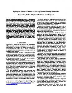
Fig. 2: Box-Whisker plots using BAM and BFM values using two standard datasets; (a) (b) the values of BAM and BFM [16] using Bonn University dataset [11] and (c) (d) Freiburg University Hospital dataset [15].

2 Proposed Method

Fig. 1: Samples of seizure/non-seizure dataset [11] and ictal and interictal dataset [15] where the first two rows and last two rows indicate that the non-seizure/seizure and ictal/interictal signals respectively.

Compared to the existing methods, the main contributions are: (i) a novel approach is proposed for the first time in our knowledge by exploiting temporal correlation within an EEG signal to find the transition of an event such as seizure; (ii) the proposed technique is a generic technique to achieve superior classification results for detecting seizure from ictal and interictal EEG signals consistently in terms of all crucial criteria such as accuracy, specificity, sensitivity with reduced computational time for different brain locations and datasets; (iii) we clearly differentiate interictal and ictal EEG signals in the large dataset [15] to understand the features and behavior of them; (iv) we identify the reason of the limitations of the existing method [16] in the dataset [15], and (v) we remove the artifacts of the dataset and then apply the proposed methods and existing method for result comparison purpose.

(a)

(b)

(c)

(d)

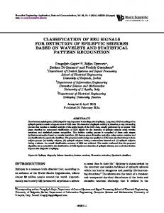
Bajaj et al. [16] used BAM and BFM features extracted from EMD for seizure and non-seizure EEG signals classification using Bonn University dataset [11]. Fig. 2(a) and (b) show Box-Whisker plots of BAM and BFM for seizure (S) and nonseizure (NS) EEG signals using the first IMF. The Box contains 50% of data distribution in the middle (i.e., the data range from Q1 to Q3); on the other hand, the Whisker contains remaining 50% of the data distribution (i.e., the data range from minimum to Q1 and from Q3 to maximum). It can be easily observed from Fig. 2 (a) and (b) that the portions of BAM and BFM of seizure signals are not overlapped with non-seizure signals. Thus, BAM and BFM could be an excellent feature to classify seizure and nonseizure EEG signals taken from Bonn University dataset [11]. As a result Bajaj et al. [16] obtained up to 100% classification accuracy for Bonn University dataset [11]. However, Fig. 2(c) and (d) show that the data ranges of BAM and BFM of interictal EEG signals are almost completely overlapped with the data ranges of ictal EEG signals while we use the EEG signals from Freiburg University Hospital [15]. Thus, BAM and BFM could not be good features for classification of the ictal and interictal signals of the dataset in [15]. However, as the IMF represents distinguishing characteristics of ictal and interictal signal separation, one of our proposed methods uses IMF for different features extractions by exploiting temporal correlation. We firstly introduce the limitations of the popular features used in the recent research to classify EEG signals, secondly derive a number of crucial characteristics by exploiting temporal correlation, and finally identify the distinguishable frequency component from decomposed/transformed signals for the extraction of features. For feature extractions, we apply DCT on three minutes ictal and interictal signals where each signal having 256Hz sample rate. For clear visualization only first 200 DCT coefficients from last quarter of coefficients are shown in Fig. 3. The figure confirms that the magnitude of high frequency coefficients is larger for ictal signal compared to that of interictal signal. Since the variance of a signal is reflected into the high frequency DCT coefficients, our hypothesis is that the characteristic (i.e., magnitude differences) of high frequency DCT coefficient can be a good feature to distinguish ictal signal from interictal signals. Note that EEG signal has non-stationary nature [22]. If we use recorded data for a time window and use DCT coefficient characteristics, we can avoid the effect of non-stationary characteristics of EEG signal analysis.

Fig. 3: DCT coefficients of ictal and interictal data from Frontal lobe for high frequency areas; the first row shows high frequency DCT coefficients of an EEG signal during ictal period of patient one, and the second row shows high frequency DCT coefficients of an EEG signal during interictal period of patient one.

In this paper, we propose a classification technique using a feature namely energy from the high frequency DCT coefficients considering temporal correlation and then classify ictal and interictal signals using LS-SVM. We also propose another technique by taking STD of raw EEG signals and STD of IMF after forming 2D matrix to exploit temporal correlation of the signals. In this experiment, it has been used the dataset [15] of 12 patients from ictal and interictal data of Frontal and Temporal lobe. To validate the proposed techniques against the existing technique, we also use the seizure and non-seizure dataset [11]. Details description of datasets is given in the Section 2.1. Details procedure of feature extractions is provided in the Section 2.3 and 2.4 while classification is provided in Section 2.6.

It means that the first portion of the signal is pre-ictal signal and the last portion is the actual seizure in our ictal signals. We do not put any explicit restriction on the duration of the seizure in our technique for classification purpose. We understand that sometimes the epoch length of the proposed techniques is shorter than the actual ictal period. The classification accuracy of the proposed techniques should not hamper too much in this situation as the pre-ictal period has also similar characteristics of the actual ictal signals as we take the pre-ictal signals from the immediate before the actual ictal signals. To make equal size (i.e., three minutes) of interictal signal with the ictal signal, we also take three minutes from each interictal signal of the dataset. Three minutes are taken from the 7th minutes of an interictal signal. The representations of the ictal and interictal signals from the dataset in [15] are in the last two rows in Fig 1. For verification purpose we also use another dataset [11]. The dataset consists of five subsets, each subset contains 100 single-channels recoding, and each recoding has 23.6 seconds in duration captured by the international 10–20 electrode placement scheme i.e., 32 electrodes at 173.61 Hz. Among them two subsets are taken from health volunteers with surface (i.e., scalp) EEG and three subsets are taken from intracranial EEG including two subsets are seizure free intervals and another subset are during seizure period (see sample examples in the first two rows in Fig 1). Note that the intracranial EEG signals have very different timefrequency characteristics compared to surface EEG.

2.1 Dataset The data in the dataset were recorded at Epilepsy centre of the University Hospital of Freiburg, Germany [15]. The data obtained by Neurofile NT digital video EEG system with 128 channels, 256Hz sampling rate, and 16 bit analogue-todigital converter. Data recording temporarily paused after each block due to technical reasons and pause time 1-3 seconds. For each of the patients, there are datasets called ictal and interictal. Firstly, system containing epileptic seizures file with 50 min pre-ictal data. Later on, it was containing 24h of EEG recoding without seizure activity. The ictal periods were determined based on identification of typical seizure patterns of experienced epileptologists. In our experiment, we use ictal and interictal dataset of Frontal and Temporal lobe along 12-patients with 3-minutes duration. Normally duration of an ictal period is from 3 seconds to 2 minutes. The signals immediate before and immediate after ictal signal are named as pre-ictal and postictal respectively. The characteristics of pre-ictal signals are very similar to the ictal signals if the pre-ictal signals are taken from the immediate before the actual ictal signals. To cover 3 minutes ictal period, we take pre-ictal signal to fill up the rest to make 3 minutes ictal signal in our experiment.

Fig. 4: Applying ICA to remove artifacts from EEG signals. First column show ictal signals from patient 1, patient 14 and patient 15 with artifact. Second column show corresponding signals without artifact.

2.2 Pre-processing The intention of data pre-processing is to improve the levels of signals of interest, while attenuating irritation or even rejecting some unwanted signals in the recordings that are marked as artifacts. Blind source separation (BSS) technique is based on statistical independent that estimates a set of source signals (i.e., physiological activity of EEG

signals) from the unknown mixture of the sources. ICA is a BSS-based approach that is useful to separate unwanted signals from EEG signals [23]. ICA is emerged as a novel and promising new tool for performing artifacts (i.e., muscle activity, eye blinks and electrical noise) corrections on EEG signals [19]-[21][24]. Two automatic artifact removal techniques are proposed in [25][26] respectively based on ICA. We apply FastICA [27] on the EEG signals to remove artifact before feature extractions of the proposed method and the existing techniques. In our experiment we use manual artifact removal process provided by [19] after applying FastICA based on the artifact information provided by the dataset [15]. Original EEG signals (x) are recorded from different electrodes and then apply ICA to compute time courses of activation (i.e., y=Wx). Note that inverse of W represents the projection strengths of the respective components onto the scalp sensors. The scalp topologies provide the information about the location of the source [19]. Corrected signals are then derived by artifactual components set to zero. Fig. 4 shows the original signal with artifacts. Corrected EEG signal is then obtained using 𝑥 ′ = 𝑊 −1 𝑦 ′ where 𝑦 ′ is the corrected activation based on the artifactual information (see second column of Fig. 4). Note that the signals are corrected using all six channels together of a patient; however, we provide an original and its corresponding corrected EEG signal of a patient in Fig. 4. 2.3 Feature Extraction using DCT DCT is a transformation method for converting a time series signal into basic frequency in such a way that the DCT coefficients are arranged from low frequency to high frequency components. Low frequency components represent the coarse signals and high frequency components represent the detail signals. As the ictal and interictal EEG signals have different amplitude and frequency (not visually separable), thus the most distinguishable features should be located in the high frequency components of DCT coefficients (see in Fig. 5). As the EEG signal is nonstationary in nature [15][22], thus, for real time processing of EEG signals, DCT may not be correct to directly correspond to the frequency analysis, however, if we segment the EEG signals in time window and apply DCT on them to find DCT coefficients; we can avoid nonstationary nature of the signals.

Fig. 5: High DCT coefficients of ictal and interictal signals with the extracted features; the first raw represents the high DCT coefficients from the ictal and interictal signals of Frontal lobe; second raw represents energy of the last quarter of DCT coefficients of ictal and interical EEG signals.

To find high frequency components, we can use 1D-DCT or 2D-DCT and then find the features e.g., energy. To see the strength of short and long term correlation, we conduct an experiment using ictal and corresponding interictal signal. In the first case we take a 15 sec epoch and apply 1D-DCT and calculate energy using last 25% of DCT coefficients (i.e., high frequency component). In the second case, we take 15 sec epoch, arrange them into 2D matrix, apply 2DDCT, and calculate energy using last 25% of DCT coefficients (i.e., high frequency component after rearranging coefficients using zigzag [32]). Then we differentiate the energy of ictal and corresponding interictal signals and draw a figure for 20 signals. Fig. 6 shows that 2D-DCT provides more energy difference between ictal and interictal signals compared to 1D-DCT for all signals. This means that the temporal correlation provides more distinguishing features. Moreover, we observe that 2DDCT-based method provides better classification results compared to 1D-DCT-based method. Thus, we use 2DDCT in the proposed technique. In this paper we mean 2DDCT when we apply DCT for 2D matrix.

Fig. 6: Energy difference between ictal and interictal EEG signals using 1D-DCT and 2D-DCT.

Energy is determined using of high DCT coefficients of each block as high DCT coefficients carrying distinguishable features to classify ictal and interictal EEG signals (see in Fig. 5). Note that the energy provides the strength of the signal. For ictal, the value of energy is normally higher compared to that of interictal signal as shown in Fig. 5. The features of energy are used as input of the LS-SVM classifier for ictal and interictal classification. The process diagram of the proposed method is presented in Fig. 7. Energy is defined as: n 2 (1) Energy   X i (t ) i 1

where n is the length of signal, X(t) is the higher frequency components of the EEG signal x(t).

Fig. 7: Process diagram of energy feature extraction using DCT.

The features extraction process using DCT is summarized as follows: i. Take three-minute EEG signal from each channel and divide into 15 second blocks. ii. Then divide each block again into 0.5 second subblock to form a matrix for exploiting temporal correlation. iii. Apply DCT on each matrix and form a 1D using zigzag manner. iv. Take 25% of high frequency DCT coefficients and calculate energy using equation (1). v. Repeat the procedure from (ii) to (iv) until end of available sub-blocks of a signal. vi. Calculate average value from energy. Note that mean value of energies from different epochs have distinguishable characteristics for ictal and interictal EEG signal classification (see in Fig. 8 for energies). vii. Repeat the procedure from (i) to (vi) until end of available signals.

Fig. 8: Mean value of energies of high frequency DCT coffients for ictal and interictal EEG signals.

Normal tendency of DCT coefficients is that the magnitude of high frequency DCT coefficients is smaller compared to low frequency DCT coefficients for a typical signal. For better understanding of the EEG signals characteristics, we investigate the tendency of DCT coefficients for different epochs (i.e., length of sub-blocks in time) to see the periodicity of the EEG signals. The Fig. 9 shows the ratio of high frequency DCT coefficients and low frequency DCT coefficients (i.e., energy of high frequency DCT coefficients divided by energy of low frequency DCT coefficients) for different epochs. The figure reveals that the ratio does not change too much for different epochs. This phenomenon indicates that the EEG signals are not periodic (or the periodicity is much larger than 2.5 seconds if they have any). Otherwise, the energy of high frequency DCT coefficients will be zero or near zero or the ratio of high to low energy would be zero. Moreover, literature including [16][22] confirm that EEG signals are non-stationary. Thus, in our case, temporal correlation exploitation by arranging 2D matrix of EEG signals is an effective way for EEG signal classification.

2.4 Feature Extraction from IMF using EMD The main strength of EMD is its ability to analyze nonstationary signals like EEG signals. EMD can successively separate the intrinsic oscillatory modes of signal into a finite number of IMFs in ordered from highest frequency component to the lowest frequency components. The number of IMFs in a signal depends on the local characteristics of the signal rather than pre-defined number of IMFs. The IMFs are the representations of different frequencies/amplitudes of the original signal and the distinguishing features between ictal and interictal EEG signals lie on the frequency/amplitude, thus, any feature extracted from IMFs will be an effective feature to classify ictal and interictal signals successfully. We observe that the ictal and interictal signals are deferred in higher order frequency components, thus our other theory is that features extracted from the first few IMFs should be enough to classify ictal and interictal signals successfully.

repeat the procedure from step (i). After generating the final IMF, the decomposition of original signal, can be written [15] as: x(t ) 

n  ci (t )  rn (t ) i 1

(2)

where n is the number of IMFs, is the ci(t) IMF and rn(t) is the final residue.

Fig. 9: Tendency of high/low frequency DCT coefficients against different epochs.

Each IMF satisfies two following conditions: (i) the number of extrema and the number of zero crossing are identical or differ at most by one and (ii) the mean value between the upper and the lower envelope is equal to zero at any time. Fig. 10 shows five IMFs from an ictal signal of Frontal lobe. Fig. 11: STD on raw EEG signal and its first IMF. Ictal signal carries higher distribution than that of interictal signal.

Bajaj et al. [16] extracted BAM and BFM from an IMF of a signal and used as features for classification. As we mentioned earlier (see the first paragraph of Section 2), the data ranges of BAM and BFM in the ictal and interictal signals are significantly overlapped, thus, the BAM and BFM features could not provide good classification results. However, we use IMF to extract different kinds of statistical features in the proposed method as the IMF represents distinguishing characteristics for the separation of ictal and interictal signals. For ictal, the value of STD is normally higher compared to that of interictal signal as shown in Fig. 11. Fig. 12 shows the process diagram of the proposed method and Fig. 11 confirms that STDs from different scenarios for ictal and interictal are a good distinguishing feature. The extracted STDs are used as input for classifier to classify ictal and interictal signals. Fig. 10: Five IMFs of ictal signal using dataset from Frontal lobe.

The features extraction using STD on raw signal and IMF is summarized as follows:

The EMD algorithm can be summarized as follows: i.

Extract the extrema (minima and maxima)of the signal

x(t ). ii.

Interpolate between minima and maxima to obtain  min (t ) and  max (t ) .

iii. Calculate local mean m(t )   min (t )   max (t ) /2 . iv. Extract the detail d (t )  x(t )  m(t ) . v.

Check d (t ) is an IMF according to the conditions which are mentioned above. If yes, repeat the procedure from step (i) on the residual signal r (t )  x(t )  m(t ) . If no, replace x(t ) with d (t ) and

i. Take three-minute EEG signal from each channel and calculate IMFs using EMD method. ii. Select an IMF and divide into 15 second blocks. Or select same three minute original/raw EEG signal and divide into 15 seconds blocks. iii. Then, divide each block again into 0.5 second subblocks to form a matrix for exploiting temporal correlation. iv. Firstly, apply STD on rows and then apply STD on a column. v. Repeat the procedure from (ii) to (iv) until end of available sub-blocks of a signal.

vi. Calculate average value from STD value of raw signal and an IMF separately. Note that mean value of STD on raw and decomposed IMF from different epochs have distinguishable characteristics for ictal and interictal EEG signal classification (see in Fig. 13 for STD on decomposed IMF). vii. Repeat the procedure from (i) to (vi) until end of available signals.

EMD-based technique as both use EMD for IMF determination. We also conduct experiment by combining the features extracted from EMD and DCT for classifications. The experimental results show that the technique with combined features does not provide better classification results compared to the proposed techniques. Moreover, any feature extraction technique using EMD takes relatively larger computational time compared to DCT. Thus, we do not include any results by combing features from DCT and EMD in the experiment. 2.6 Classification

Fig. 12: Process diagram of feature extraction from Raw signals and IMFs using STD.

Fig. 13: Mean value of STD of the first IMF for ictal and interictal EEG signals.

2.5 Computational Complexity Feature extractions using IMF through EMD take longer time due to two fold iterations to find all IMFs. In the first iteration EMD decomposes a signal and checks whether the signal makes an IMF and in the second iteration it subtracts the current IMF from the signal and continues for the next IMF. Even if we stop the iteration for the first IMF, the EMD-based technique takes a full first iteration for calculating the IMF. The experimental data reveals that the proposed technique using DCT takes less computational time compared to the EMD-based technique as DCT transformation is faster compared to the EMD decomposition. On the other hand, the proposed second technique takes similar computational time compared to the

The goal is to find patients states, ictal (Class 1) and interictal (Class 2) using the machine learning approaches through cross-validation evaluation. The challenge is to find the mapping that generalized from training sets and unseen test sets. For the cross-validation, data are partitioned into training set and test set [28]. To classify the ictal and interictal signals, we extract features from DCT and IMF. For classification, we use LS-SVM [18] classifier as the LS-SVM is one of the best classifiers in the EEG signal analysis. It can minimize the operational error and maximize the margin hyperplane, as a result it will maximize the classification performance [29][30]. For non-linear problem the kernel function is introduced in the decision function can be defined: N  f ( x)  sign  i yi K ( x, xi )  b (3) i  1   where K(x, xi) is a kernel function,  i is the Lagrange multipliers [31], b is the bias term, and yi the training output pairs. RBF kernel is used in our experiments and this function can be defined as: 2 (4) k ( x, xi )  exp  x  xi / 2 2    where σ controls the width of the RBF function.

3 Experimental Results The method in [16] is considered as the state-of-the-art method because it is the latest and high accurate method in our knowledge for the classification of seizure and nonseizure signals using dataset [11]. To verify the strength and weakness of the proposed methods in terms of accuracy, specificity, sensitivity, and computational times, we compare the proposed methods with the relevant and latest existing method [16] using different datasets for detecting the seizure from different types of other epileptic signals. In the proposed DCT based method, we apply the 2D-DCT to exploit temporal correlation in the datasets [11][15] and take the higher frequency components to generate energy. Energy can distinguish ictal and interictal information according to the nature of amplitude. In another proposed method, we use STD of raw signals and STD on IMFs

features to get classification benefit by exploiting temporal correlation of the EEG signals. In the paper, we use different signal processing transformation/decomposition techniques. After transformation/decomposition of the signals, we learn and observe different characteristics of the EEG signals in time and frequency domains which are further processed for feature extraction and then used to classify ictal and interictal EEG signals. The novelty of the signal processing is described below: (i) As EEG signal is non-stationary, our hypothesis is that temporal correlation within a signal would be a good indicator to detect a transition from one event to another event (in this case seizure and non-seizure). Thus, we derive a novel approach for the first time in our knowledge by exploiting temporal correlation within an EEG signal to find the transition of an event such as seizure. (ii) To detect the seizure from non-seizure signals with higher accuracy, we use a number of statistical features from the original signals without changing their original domain and the transformed/decomposed signals with changing their original domain and extracting distinguishing characteristics. This strategy also provides superior classification results for detecting seizure from ictal and interictal EEG signals consistently in terms of all crucial criteria such as accuracy, specificity, sensitivity with reduced computational time for different brain locations and datasets. For all techniques, we classify the ictal and interictal (or non-seizure) data extracted from Frontal and Temporal lobe signals using LS-SVM classifier with RBF kernel. In our experiment, we randomly select 80% in the training set and established an LS-SVM model in the learning phase and remaining 20% of the original set to check the model is well fit. When the dataset is trained through LS-SVM then classification is performed by testing with testing dataset. After testing the performance is evaluated by computing sensitivity, specificity and accuracy [16]. Sensitivity (also called recall rate in some fields) measures the proportion of actual positives which are correctly identified, thus, in our case sensitivity is determined from the ictal signals. Specificity measures the proportion of negatives which are correctly identified, thus, specificity is determined from the interictal signals. Accuracy indicates overall classification performance. Table 1 shows the sensitivity, specificity and accuracy results of classifications using two proposed methods against the state-of-the-art method [16]. The technique in [16] claims that the second IMF provides better classification results while they use BAM and BFM features for the dataset in [11]. We conduct experiments using first four IMFs, however, we provide results using only first IMF in Table 1. It can be observed from Table 1 that the proposed

two methods (energy from DCT) and (STD from raw EEG signals and decomposed IMF) outperform the state-of-theart method [16] in terms of sensitivity (i.e., represent the ictal signals) and accuracy for Frontal lobe signals. In the Frontal lobe signals, DCT based energy features contains 100% sensitivity, 96.68% specificity and 97.32% accuracy whereas the classification performance of sensitivity is 47.88%, specificity is 85.67% and accuracy is 79.94% for the state-of-the-art method [16]. According to the experimental results using Temporal lobe, the proposed method based on IMF does not provide good results in terms of accuracy (i.e., combined of ictal and interictal) and specificity (i.e., accuracy of interictal only) compared to the state-of-the-art method [16]; however, it provides perfect results (100%) in terms of sensitivity (i.e., accuracy of ictal identification). Normally the cost of failure of detecting ictal is higher compared to the interictal. Thus, in this view, the proposed method outperforms the existing method. Beside this, the proposed method based on DCT outperforms the existing method comprehensively by providing excellent results in terms of accuracy, sensitivity, and specificity where they are more than 96% for all cases. Table 1: Sensitivity, specificity and accuracy comparison using different techniques for ictal and interictal EEG signals from Frontal lobe; BAM and BFM from technique in [16]; energy feature from high frequency DCT coefficients in the first proposed method; and STD of raw EEG singals and STD on IMF features from EMD. Brain Location

Criteria

Existing Method EMD BAM and BFM[15]

Frontal Lobe Temporal Lobe

SEN SPE ACC SEN SPE ACC

47.88 85.67 79.94 55.20 86.45 86.14

Proposed Methods IMF Features STD on Raw and Decomposed signals 100 81.08 81.33 100 81.00 82.00

DCT Energy

100 96.68 97.32 100 97.31 97.86

To see the worthiness of the above mentioned atrifacts removal process, we test the capability of the proposed DCT-based technique without FastICA-based atrifacts removal procedure. In this case, we get 24.06% sensitivity, 82.97% specificity and 76.87% accuracy for DCT based method using Frontal lobe. Compared to the results in Table 1, it can be easily observed that the proposed DCT-based technique provides better results for EEG signals without artifacts. To get the clear picture, we also investigate our techniques using the dataset [11]. To extract the features using DCT, we reshape a 23.6 seconds EEG signal into a two dimensional feature vectors to exploit temporal correlation of the raw EEG signals by diving the signal into 3 seconds block (i.e., total 7 epochs for a signal). Then, each block is again divided into 0.5 second sub-block. The sub-blocks are arranged into a 2D matrix to exploit temporal correlation. Then apply DCT on each 2D matrix for all blocks individually. Energy are determined using 25% of high

(a)

(b)

Fig. 14: Visual classification of ictal and interictal EEG signals from Frontal lobe for testing subsets; left column represents the classification results from Frontal lobe using the first IMF of the existing method [13] and right column represents the proposed IMF-STD-based method (right column).

DCT co-efficient of each block as high DCT coefficients carrying distinguishable features to classify seizure and non-seizure EEG signals. The proposed technique based on DCT, we get 98.91%, 94.35%, and 95% sensitivity, specificity, and accuracy respectively. Thus, we believe that the comparison is meaningful as the experimental results reveal that the proposed methods is not good enough for the dataset in [11] compared to the technique in [16] but the proposed methods outperforms the technique in [16] using the dataset in [17]. Moreover, the proposed technique is consistent in terms of accuracy, sensitivity, specificity, and computational time using different datasets and brain locations. Thus, the proposed method is a generic scheme with better consistent for wider ranges of datasets, brain locations and performance. Fig. 14 shows the visual classification comparison using the proposed methods and the state-of-the-art method [16] for better understanding using the dataset in [15]. We generate left column image in Fig. 14 from Frontal lobe for the first IMF of testing set and obtain the classification accuracy 79.94% by the existing method [16] (see left column of Fig. 14) and 81.33% by the proposed IMF-based method (see right column of Fig. 14). Moreover, visually we can see from Fig. 14 that the existing method has more miss-classified ictal signals (see first column) compared to that of the proposed methods. Thus, it can be concluded from Fig. 14 that the proposed methods outperform the state-of-the-art method using the dataset in [15]. The performance of the LS-SVM is evaluated by receiver operating characteristics (ROC) plots is shown in Fig. 15 using the dataset in [15]. ROC demonstrated the performance of a binary classifier system where it is created by plotting the fraction of true positives from the positives i.e., true positive rate (TPR) vs. the fraction of false positives from negatives i.e., false positive rate (FPR) with various threshold settings. TPR can represent as sensitivity, and FPR is one minus the specificity or true negative rate.

Fig. 15 demonstrate that the proposed methods based on DCT and IMF provide good classification results than that of the existing [16] method.

Fig. 15: The receiver operating characteristics (ROC) curve of of training and testing EEG signals using LS-SVM with RBF kernel from Temporal lobe.

4 Conclusion We propose a new approach based on energy features from high frequency DCT coefficients to exploit temporal correlation of the EEG signals to classify ictal and interictal EEG signals using LS-SVM classifier. The magnitude of high frequency DCT coefficients for ictal and interictal signals is different, thus, energy extracted from high frequency DCT coefficients is good features to distinguish ictal and interictal signals. We also propose another method by using two features namely STD of raw signals and STD of decomposed IMF for better classification. The experimental results show that the proposed methods outperform the state-of-the-art method for Frontal and Temporal lobe signals in terms of sensitivity for ictal and interictal signals classification. Moreover, the proposed

methods perform more consistently in terms of sensitivity, specificity, and accuracy compared to the existing state-ofthe-art method for the seizure and non-seizure dataset.

References [1]

[2]

[3]

[4]

[5]

[6]

[7]

[8]

[9]

[10]

[11]

[12]

[13]

[14]

[15]

[16]

[17]

[18]

[19]

M. Soleymani, T. Pun, and M. Pantic, "Multi-Modal Emotion Recognition in Response to Videos", IEEE Transactions on Affective Computing, 2012, 3(2): p. 211-223. S. Scholler, S. Bosse, M. S. Treder, B. Blankertz, G. Curio, K.-R. Müller, and T. Wiegand,” Toward a Direct Measure of Video Quality Perception Using EEG”, IEEE Transactions on Image Processing, May 2012, 21(5): p. 2619-2629. W. Di, C. Zhihua, F. Ruifang, L. Guangyu, and L. Tian, “Study on human brain after consuming alcohol based on EEG signal,” International Conference on Computer Science and Information Technology (ICCSIT), 2010, 5: p. 406 – 409. E. Estrada, H. Nazeran, F, Ebrahimi, and M Mikaeili, “EEG signal features for computer-aided sleep stage detection”, IEEE EMBS conference on neural engineering, 2009, p. 669 - 672. Z. M. Hanafiah, K. F. M. Yunos, Z. H. Murat, M. N. Taib, S. Lias, “ EEG brainwave pattern for smoking behaviour after horizontal rotation treatment”, IEEE student conference on research and development, 2009, p. 559 - 561. Z. H. Murat, R. Shilawani, S. A. Kadir, R. M. Isa, and M N. Taib, “The effects of mobile phone usage on human braingwave using EEG”, International conference on modeling and simulation, 2011, p. 36-41. Panda, P.S. Khobragade, P.D. Jambhule, S. N. Jengthe, P. R. Pal, and T. K. Gandhi, “Classification of EEG signal using wavelet transform and support vector machine for epileptic seizure diction,” International Conference on Systems in Medicine and Biology (ICSMB), 2010, p. 405-408. S. G. Dastidar, H. Adeli, and N. Dadmehr, “Mixed-band wavelet chaos-neural network methodology for epilepsy and epileptic seizure detection,” IEEE Transactions on Biomedicine Engineering, 2007, 54(9): p. 1545-1551. H. Ocak, “Optimal classification of epileptic seizures in EEG using wavelet analysis and genetic algorithm,” Signal Processing, 2008, 88(7): p. 1858-1867. K. Polat and S. G¨unes, “Classification of epileptiform EEG using a hybrid system based on decision tree classifier and fast Fourier transform,” Applied Mathematics and Computation, 2007, 187(2): p. 1017-1026. EEG time series data, Department of Epileptology, University of Bonn, Available at http://epileptologiebonn.de/cms/front_content.php?idcat=193&lang=3&changelang=3, Visited Date: April 28, 2012. R. B. Pachori, “Discrimination between ictal and seizure-free EEG signals using empirical mode decomposition,” Research Letters in Signal Processing, Article ID 293056, 2008. R. B. Pachori and V. Bajaj, "Analysis of normal and epileptic seizure EEG signals using empirical mode decomposition", Computer Methods and Programs in Biomedicine, 2011, 104(3): p. 373-381. V. Bajaj and R. B. Pachori, "Epileptic seizure detection based on the instantaneous area of analytic intrinsic mode functions of EEG signals", Biomedical Engineering Letters, 2013, 3(1): p. 17-21. EEG Data set from Epilepsy Center of the University Hospital of Freiburg, http://epilepsy.uni-freiburg.de/freiburg-seizure-predictionproject/eeg-database, Visited Date: June 10, 2012. V. Bajaj and R. B. Pachori, “Classification of Seizure and Nonseizure EEG Signals using Empirical Mode Decomposition,” IEEE Transactions on Information Technology in Biomedicine, 2012, 16(6): p. 1135-1142. J. R. Williamson, D. W. Bliss, D. W. Browne, and J. T. Narayanan, “Seizure prediction using EEG spatiotemporal correlation structure,” Epilepsy and Behavior, 2012, 25(2): p. 230-238. J. A. K. Suykens and J. Vandewalle,” Least Squares Support Vector Machine Classifiers,” Neural Processing Letters, 1999, 9(3): p. 293– 300. TP. Jung, S. Makeig, C. Humphries, et al., “Removing electroencephalographics artifacts by blind source separation,” Society for Psychophysiological Research, 2000, 37(2): p. 163-178.

[20] W. De Clercq, A. Vergult, B. Vanrumste, W. V. Paesschen, S. V. Huffel, “Canonical Correlation Analysis Applied to Remove Muscle Artifacts From the Electroencephalogram,” IEEE Transactions on Biomedical Engineering, 2006, 53(12): p. 2583-2587. [21] J. Ma, P. Tao, S. Bayram, V. Svetnik, “Muscle artifacts in multichannel EEG: characteristics and reduction,” Clinical Neurophysiology, 2012, 123(8): p. 1676-1686. [22] S. Mihandoost, M. Amirani, M. Mazlaghani, and A. Mihandoost, “Automatic feature extraction using generalised autoregressive conditional heteroscedasticity model: an application to electroencephalogram classification,” IET Signal Processing, 2012, 6(9): p. 829-838. [23] D. Gupta, C. J. James, and W. P. Gray,” Phase synchronization with ICA for epileptic seizure onset prediction in the long term EEG,” IET International Conference on Advances in Medical, Signal and Information Processing (MEDSIP), 2008, p. 1-4. [24] A. Hyvärinen, and E. Oja, Independent component analysis: algorithms and applications. Neural Networks, 2000. 13(4–5): p. 411430. [25] P. LeVan, E. Urrestarazu, and J. Gotman, A system for automatic artifact removal in ictal scalp EEG based on independent component analysis and Bayesian classification. Clinical Neurophysiology, 2006. 117(4): p. 912-927. [26] Romo Vázquez, R., et al., Blind source separation, wavelet denoising and discriminant analysis for EEG artefacts and noise cancelling. Biomedical Signal Processing and Control, 2012. 7(4): p. 389-400. [27] Aalto University, “Independent Component Analysis (ICA) and Blind Source Separation (BSS), The FastICA package for MATLAB,” URL: http://research.ics.aalto.fi/ica/fastica/, visited date 6 June 2014. [28] H. Xing, M. Ha, B. Hu, and D. Tian, “Linear feature- weighted support vector machine,” Springer and Fuzzy Information and Engineering Branch of the Operations Research Society of China, 2009. [29] H. Wang and D. Hu,” Comparison of SVM and LS-SVM for Regression,” International Conference on Neural Networks and Brain, 2005, p. 279 – 283. [30] K. D. Brabanter, P. Karsmakers, F. Ojeda, C. Alzate, J. D. Brabanter, K. Pelckmans, B. De Moor, J. Vandewalle, and J.A.K. Suykens, LSSVM Lab Toolbox User’s Guide, version 1.8, Katholieke Universiteit Leuven, 2011. [31] M. Paul, M. Frater, and J. Arnold, “An Efficient Mode Selection Prior to the Actual Encoding for H.264/AVC Encoder,” IEEE Transactions on Multimedia, 2009, 11(4): p.581-588. [32] M. Paul, C. Evans, and M. Murshed, “Disparity-adjusted 3D multiview video coding with dynamic background modeling,” IEEE International Conference on Image Processing, pp. 1719-1723, 2013.