Equality Set Projection: A new algorithm for the ... - Infoscience

Equality Set Projection: A new algorithm for the projection of polytopes in halfspace representation Colin N. Jones, Eric C. Kerrigan and Jan M. Maciejowski CUED/F-INFENG/TR.463 June 8, 2004

Equality Set Projection: A new algorithm for the projection of polytopes in halfspace representation Colin N. Jones, Eric C. Kerrigan and Jan M. Maciejowski Department of Engineering University of Cambridge Cambridge CB2 1PZ United Kingdom {cnj22, eck21, jmm}@eng.cam.ac.uk Technical Report CUED/F-INFENG/TR.463 June 8, 2004

Abstract In this paper we introduce a new algorithm called Equality Set Projection (ESP) for computing the orthogonal projection of bounded, convex polytopes. Our solution addresses the case where the input polytope is represented as the intersection of a finite number of halfplanes and its projection is given in an irredundant halfspace form. Unlike many existing approaches, the key advantage offered by ESP is its output sensitivity, i.e., its complexity is a function of the number of facets in the projection of the polytope. This feature makes it particularly suited for many problems of theoretical and practical importance in which the number of vertices far exceeds the number of facets. Further, it is shown that for non-degenerate polytopes of fixed size (dimension and number of facets) the complexity is linear in the number of facets in the projection. Numerical results are presented that demonstrate that high dimensional polytopes can be projected efficiently.

1

Introduction

Polytopes provide a useful representation for the linear constraints that appear in diverse fields such as control, finance and optimisation. The calculation of the orthogonal projection of a polytope is a fundamental operation that arises in many applications. For example, in control theory, projection is required for reachability analysis [6] and in decision theory for the elimination of existential quantifiers [17]. It can be shown that the calculation of affine maps or Minkowski sums of polytopes are both equivalent to orthogonal projection [11], making a projection algorithm a necessary tool for working with polytopes. It is well known that polytopes can be represented in two forms: as the convex combination of a finite number of vertices and as the intersection of a finite number of halfspaces. For any d-dimensional polytope, represented as the intersection of q halfspaces, the number of 1

vertices required to describe the same polytope is O(q b 2 c ) in the worst case. Polytopes that d

exhibit an exponential relationship are common in various fields. For example, a hypercube in d-dimensions can be described by 2d halfspaces or 2d vertices. Vertex representation is appropriate in some applications, while in others halfspace is preferred. In this paper, we are interested in polytopes that are in halfspace representation and whose projection should also be given in halfspace form. As the vertex representation of the given polytope can be exponentially more complex than the halfspace representation, we ideally want the complexity of the projection algorithm to depend only on the number of halfspaces, and never to compute the vertices. As the effects of this exponential behaviour do not become significant until the dimensionality of the problem is large, this algorithm is most suited to the projection of high dimensional polytopes. In this paper we give a new algorithm, dubbed Equality Set Projection (ESP), for the computation of the projection of a bounded polytope described as the intersection of a finite number of halfspaces in arbitrary dimension. We do not make the assumption that the polytope is in general position or that the description is irredundant, although the description of the projection returned by the algorithm is irredundant. It will be shown that for a polytope of fixed size (dimension and number of halfspaces), ESP computes the projection using a number of linear programs that is linear in the number of halfspaces in the projection.

1.1

Related Work

We briefly review the literature on projection methods and examine its relation to our work. Current projection methods that can operate in general dimensions can be grouped into three classes: Fourier elimination, block elimination and vertex based approaches. While each approach can be effective for a particular class of polytopes, there is as yet no algorithm whose complexity is a function of the number of halfspaces required to describe the projection. Here, we give a brief overview of these approaches and their derivatives. Fourier-Motzkin elimination was originally described by Fourier in 1824 and has been improved many times since. This approach can be thought of as the analogue of Gaussian elimination for linear inequalities. At each iteration of the algorithm the polytope is recursively projected by one dimension until the desired dimension is reached. The primary limitation of Fourier-Motzkin elimination is that it generates many redundant constraints at each iteration. It is not practical to remove the redundancies at each step, although modˇ ifications of the algorithm due to Cernikov [16] in 1963 greatly improved the efficiency by identifying many redundant constraints with very little added work. For some polytopes, algorithms based on Fourier elimination can be efficient and recent work [10] has improved the average case complexity for very sparse constraints. However, for a polytope described by q halfspaces that is to be projected down by k dimensions, the time complexity of Fourier k

elimination is O(q 2 ), often making it unusable even for small problems. 2

In [13], a modification of Fourier’s method is proposed in which a set of k + 1 constraints is selected and all k dimensions of this  set that are to be projected are removed using Gaussian elimination. There are, however,

q k+1

sets of constraints that must be considered making

this algorithm only suitable for very specific applications. The second well known approach is block elimination. In this method a polyhedron is defined called the projection cone. The extreme rays of this cone can then be used to find the defining halfspaces of the projection. Methods available for computing the extreme rays, such as the double description algorithm [8] or the reverse search approach [2], are exponential in the worst case and as with Fourier elimination, this approach may generate a large number of redundant inequalities that need to be removed. Recent work by Balas [3] has shown that if certain invertibility conditions are satisfied, then every extreme ray of the projection cone generates an irredundant constraint of the projection. This observation has been extended to polytopes that do not satisfy these conditions by the introduction of a transformation of the cone such that each ray of the projection of the transformed cone corresponds to a constraint of the projection of the polytope. The limitation of this approach is that the calculation of the extreme rays of the projection of the transformed cone may be very difficult, although it offers an important insight into the structure of projection. The final class of approaches covers a variety of methods that compute vertices of the projection. While these approaches are suitable for a certain class of polytopes, we are interested here in polytopes in which the vertices greatly outnumber the inequalities. As a result, any approach that requires the enumeration of the vertices of either the polytope or its projection can be as much as exponentially slower for this class than an approach that considers only inequalities. All vertices of the polytope can be computed using a vertex enumeration algorithm, each vertex can then be trivially projected, before a convex hull algorithm is used to calculate the inequality constraints of the projection. Vertex enumeration and convex hulls can be computed using the same algorithms (for example, [2, 8]). This approach can be efficient for polytopes with large numbers of redundant inequalities or a small number of vertices. However, as there can be exponentially more vertices than there are inequalities, the applicability is limited to polytopes with a small vertex count. A contour-tracking approach is proposed in [13] in which the skeleton of the projection is traced. The skeleton is formed from the vertices and the one-dimensional lines that join them. The complexity is a linear function of the number of vertices of the projection and as a result is suitable only when the number of vertices is small when compared to the number of inequalities. An approach, similar to that developed in this paper, was outlined in [1]. The purpose was to compute both the vertex and half-space representation of the projection, although

3

the algorithm can be adapted to compute only the inequalities if desired. Three restrictive assumptions are made, which we relax in this paper. First, in [1] it is assumed that the polytope is in general position; while there exist standard techniques to ensure that this is the case for general polytopes [7], these techniques can cause the description of the projection to increase significantly in size. Second, it is implicitly assumed in [1] that the description of the polytope is irredundant. While this requirement is not necessarily prohibitive and can be satisfied by running as many linear programs as there are constraints, it will greatly slow the algorithm if the dimension is large, or if there are many redundant inequalities. Finally, the assumption is made in [1] that every face of the polytope that projects to a facet of the projection is of dimension d − 1. While there is a class of polytopes for which this is the case, it is not true in general and we remove this assumption in this paper. The remainder of this paper is organised as follows. Section 2 provides an introduction to polytopes and their projections and introduces the notion of an equality set. Section 3 gives an outline of the ESP algorithm while Sections 4 through 6 provide the details. The complexity of the algorithm is investigated in Section 7 and numerical simulation results are reported in Section 8. Concluding remarks are made in Section 9. Appendix A details a well-known algorithm for the calculation of the affine hull of a polytope. Appendices B and C show how to modify polytopes that do not contain the origin or are not full dimensional so that their projections can be computed via ESP.

Notation If A ∈ Rm×n is a matrix, then null (A) , {x ∈ Rn | Ax = 0} and range (A) , {y ∈ Rm | ∃x ∈ Rn , y = Ax} are the nullspace and columnspace of A respectively. N(A) and R(A) are defined as matrices whose columns form an orthonormal basis for null (A) and range (A) respectively. Note that in general N(A) and R(A) are not unique. In order to ensure uniqueness, if the rank of A is r and U ΣV T is the singular value decomposition of A, then we define R(A) to be the first r columns of U and N(A) to be the last n − r columns of V . The symbol † will be used to define the Moore-Penrose pseudo-inverse. If S and U are sets, then S\U = {x | x ∈ S, x 6∈ U } is the difference operator and |S| is the cardinality of S.

2

Polytopes and Projections

This section provides an overview of projections of polytopes. The notion of an equality set will be introduced and the properties relevant to projection will be demonstrated.

4

2.1

Affine Sets and Polytopes

Vector spaces and the related notions of subspaces and affine sets are fundamental to any discussion of polytopes and therefore we begin this introduction with a brief review of these concepts. A vector space V over the reals is a set of vectors z ∈ Rn that contains the origin and is closed under vector addition and scalar multiplication. A subspace of a vector space V is any subset of L ⊆ V that is itself also a vector space. Recall that L can be represented in two common forms: as the set of all vectors satisfying a finite set of homogeneous linear equations: L = {z ∈ Rn | Az = 0} ,

for some A ∈ Rq×n

(1)

or in terms of the span of a finite set of vectors vi ∈ Rn : ) p X z ∈ Rn z = λi vi , λi ∈ R .

( L = span {v1 , . . . , vp } =

(2)

i=1

If the vectors vi are linearly independent, then the set {v1 , . . . , vp } forms a basis for L. The dimension of a subspace L ⊆ Rn , denoted dim L, is defined as the smallest number of vectors whose span is L. Note that if the subspace is defined as in (1), then the dimension can be calculated as dim L = n − rank A. If it is represented as in (2), then its dimension is the number of linearly independent vectors vi . A subset M ⊆ Rn is called an affine set if (1 − λ)x + λy ∈ M for every x, y ∈ M and λ ∈ R. Two affine sets M1 and M2 are said to be parallel if they can be written as for some a ∈ Rn .

M1 = M2 + a,

(3)

Theorem 1. [14, Thm 1.2] Each non-empty affine set M is parallel to a unique subspace L. This L is given by L = M − M = {x − y | x, y ∈ M } . Theorem 1 and (3) allow us to write every affine set M as a translate of a unique subspace L for some a ∈ Rn .

M = L + a,

(4)

The two representations of subspaces defined above give rise to two representations of affine sets. Equation 1 gives the representation in terms of all solutions of a finite set of linear

5

equations: for some a ∈ Rn

M = L + a, = {z ∈ Rn | Az = 0} + a = {z ∈ Rn | A(z − a) = 0} = {z ∈ Rn | Az = b} , Affine sets of the form

b , Aa.

(5)



z | aT z = b , a ∈ Rn , b ∈ R are called hyperplanes. Equation 5

shows that all affine sets can be written as the intersection of a finite number of hyperplanes. Given a set S ⊆ Rn , the affine hull of S, denoted aff S, is the intersection of all affine sets containing S. Clearly, the affine hull of an affine set is itself. It can be shown that the P affine hull of S consists of all the vectors y of the form y = pi=1 λi vi , such that vi ∈ S and Pp i=1 λi = 1 [14]. Equation 2 allows us to write any affine set as the affine hull of a finite number of vectors: M = L + a, ( =

z∈R

n

( =

z∈R

n

( =

z ∈ Rn (

=

z∈R

n

z z z z

=

p X

for some a ∈ Rn

) λi vi , λi ∈ R

+a

i=1

=a+

p X

) λi vi , λi ∈ R

i=1

= λp+1 a + =

p+1 X

λi µ i ,

i=1

p X

λi (vi + a),

i=1 p+1 X

p+1 X

) λi = 1, λi ∈ R

i=1

)

λi = 1, λi ∈ R

i=1

= aff {µ1 , . . . , µp+1 } , where µi , vi + a, i = 1, . . . , p, µp+1 , a. If z1 , z2 ∈ M , where M = L + a is an affine set, L is a subspace and a is a vector then z1 and z2 are called affinely independent if and only if z1 − a and z2 − a are linearly independent. This allows the notion of dimension to be extended to affine sets as follows: the dimension of an affine set M , denoted dim M , is defined as the dimension of the subspace which is parallel to it, dim M , dim L if M = L + a, where L is a subspace. A subset C ⊆ Rn is convex if (1 − λ)x + λy ∈ C whenever x, y ∈ C and 0 ≤ λ ≤ 1. Clearly, all affine sets are convex. The convex hull of a set S ⊆ Rn is the intersection of all the convex sets containing S and is denoted conv S. The convex combination of a set of P Pp vectors {v1 , . . . , vp } is all points pi=1 λi vi , i=1 λi = 1, λi ≥ 0. Theorem 2. [14, Thm 2.3] For any S ⊂ Rn , conv S consists of all convex combinations of 6

the elements of S. Corollary 3. [14, Cor. 2.4] The convex hull of a finite subset {v1 , . . . , vp } of Rn consists of P Pp all vectors of the form pi=1 λi vi , with λi ≥ 0, i=1 λi = 1.  A closed halfspace is a convex set of the form z ∈ Rn | aT z ≤ b , a ∈ Rn , b ∈ R. Any set that can be expressed as the intersection of a finite number of closed halfspaces is called a polyhedral (convex) set: P , {z ∈ Rn | Az ≤ b} ,

A ∈ Rq×n , b ∈ Rq .

The dimension of a polyhedron P is the dimension of its affine hull: dim P , dim aff P. If a halfspace constraint can be removed from the description of P without changing the polyhedron, then it is called redundant. If the description of P contains no redundant constraints, then it is called irredundant. Note that while the convex hull of a set of points is always bounded, polyhedra may not be. If a polyhedra is bounded, then it is called a polytope. Throughout the remainder of this paper, we shall assume that all polyhedra are bounded. The Minkowski-Weyl Theorem (Theorem 4 below) is fundamental as it allows a polytope to be expressed in two forms: as the intersection of a finite number of halfspaces or as the convex hull of a finite number of vectors. Theorem 4. (Minkowski-Weyl) A subset P ⊂ Rn is the convex hull of a finite set of vectors P = conv {v1 , . . . , vp } ,

where each vi ∈ Rn ,

if and only if it is a bounded intersection of halfspaces P = {z ∈ Rn | Az ≤ b} ,

for some A ∈ Rq×n , b ∈ Rq .

Efficient methods exist for converting between one representation and the other [2,8]. However, there can be an exponential relationship between the representations: if a n−dimensional n polytope can be described by the intersection of q halfspaces, it may take up to O(q b 2 c ) vertices to formulate the convex hull. Similarly, if a polytope is given as the convex hull of m vertices, an exponential number of halfspaces may be needed to describe the same object. Many applications produce polytopes that exhibit this exponential relationship. The projection method presented here operates only on the polytope in halfspace form without computing the vertex representation and so is particularly suited to polytopes that require a 7

Table 1: Face names of an n-dimensional polytope Dimension Name (n − 1)-face Facet (n − 2)-face Ridge 1-face Edge 0-face Vertex small number of halfspaces to describe them but a very large number of points to formulate as a convex hull.

2.2

Face Lattice

In this section we recall a natural decomposition of polytopes: the face lattice. Definition 5. (Face) [19, Def. 2.1] F is a face of the polytope P ⊂ Rn if there exists a  hyperplane z ∈ Rn | aT z = b , where a ∈ Rn , b ∈ R, such that  F = P ∩ z ∈ Rn | aT z = b and aT z ≤ b for all z ∈ P . Note that ∅ and P are both faces of P (consider the hyperplanes   z | 0T z = 1 and z | 0T z = 0 , respectively); all other faces are called proper faces. Theorem 6. [19, Prop. 2.2] Let P ⊂ Rn be a polytope and let F be a face of P : 1. The face F is a polytope. 2. Every intersection of faces of P is a face of P . 3. The faces of F are exactly the faces of P that are contained in F . 4. F = P ∩ aff F . Note that as each face of a polytope is itself a polytope, the notion of dimensionality applies to faces. If a face is of dimension p, then it is called a p-face. Faces of particular dimensions have explicit names as shown in Table 1. Note that for a polytope in Rn , the word face refers to a face of arbitrary dimension, while facet refers specifically to the (n − 1)-faces. Theorem 6 allows a natural partial ordering over the faces of a polytope based on inclusion. If P is a polytope, then each face of P is itself a polytope whose faces are a subset of P ’s faces. This allows us to draw a face lattice where each node represents a face of the polytope and two nodes are connected if one is a subset of the other. The lattice is organized vertically, such that faces of the same dimension appear at the same level and the dimension increases up the diagram. An example lattice of a cube is shown in Figure 1. 8

Edge Facet

Vertex

P Facets Edges/Ridges Vertices

∅

Figure 1: Face lattice of a cube

F H1

H2 G

Figure 2: Illustration of “Diamond Property” A property of the face lattice that is key to the projection method developed here is the so-called diamond property: Theorem 7. (Diamond property) [19, Thm 2.7(iii)] If G and F are faces of a polytope P and G ⊂ F with dim F − dim G = 2, then there are exactly two faces H1 , H2 with the property G ⊂ H1 ⊂ F and G ⊂ H2 ⊂ F . Note that, as the name of the proposition implies, the four faces in Theorem 7 will “look like” a diamond, as shown in Figure 2. The immediate implication of Theorem 7 is that any two facets ((n−1)-faces) of a polytope are either not joined in the face lattice or are connected by the inclusion of exactly one ridge. Two faces F1 and F2 of P are said to be adjacent if the intersection F1 ∩ F2 is a facet of both.

2.3

Equality Sets of a Polytope

We now introduce the notion of the equality set, which is the method that will be used in this paper for defining faces. If P , {z ∈ Rn | Az ≤ b} is a polytope defined by the intersection of q halfspaces and E ⊆ {1, . . . , q}, then AE is a matrix whose rows are the rows of A whose indices are in E. 9

v

4 3 1

2

Figure 3: Illustration of equality sets Similarly, bE is the vector formed by the rows of b whose indices are in E. The relevant rows of AE are taken in the same order as those of the matrix A. If E = {i} is a singleton, then we write Ai for A{i} . The notation PE refers to the set PE , P ∩ {z | AE z = bE }. Definition 8. (Equality Set) Let P , {z | Az ≤ b} be a polytope defined by the intersection of q halfspaces, E ⊆ {1, . . . , q} and G(E) , {i ∈ {1, . . . , q} | Ai z = bi , ∀z ∈ PE } . The set E is an equality set of P if and only if E = G(E). Remark 9. Note that this definition of an equality set is similar to the notion of an equality subsystem used in [4]. Whereas equality subsystems generally refer to any description of the affine set that describes the affine hull of the face, equality sets describe this affine set specifically in terms of all of the inequalities of P that are met with equality at all points in the face. To illustrate the idea of an equality set, consider the pyramid shown in Figure 3. Notice that the set P{1,2,3} is the face, or more specifically, the vertex v, but that {1, 2, 3} is not an equality set, since G({1, 2, 3}) = {1, 2, 3, 4}. There is only one equality set that defines the face v, and that is {1, 2, 3, 4}. The goal is to re-write the face lattice in terms of equality sets. First, the relationship between equality sets and faces must be made explicit: there is a one-to-one mapping between faces and equality sets. We begin with the following well-known result: equality sets define affine hulls.

10

Lemma 10. If E is an equality set of the polytope P , {z ∈ Rn | Az ≤ b}, then aff PE = {z ∈ Rn | AE z = bE } and dim PE = n − rank AE . Proof. The first result follows directly from Definition 8. The second result follows from dim PE = dim aff PE = n − rank AE . Lemma 11. (Uniqueness of Equality Sets) If E and B are equality sets of a polytope P , {z ∈ Rn | Az ≤ b}, then E = B if and only if PE = PB . Proof. Clearly, if E = B, then PE = PB . Assume that PE = PB . Since E and B are equality sets, E = G(E) and B = G(B) and because PE = PB we have E = G(E) = {i | Ai z = bi , ∀z ∈ PE } = {i | Ai z = bi , ∀z ∈ PB } = G(B) = B.

Theorem 12 proves the assertion that there is a one-to-one mapping between equality sets and faces. Theorem 12. If E is an equality set of the polytope P , {z ∈ Rn | Az ≤ b}, then PE is a face of P . Furthermore, if F is a face of P , then there exists a unique equality set E such that F = PE . Proof. If i ∈ E, then Ai z ≤ bi is true for all z ∈ P and therefore P ∩ {z ∈ Rn | Ai z = bi } is a face by Definition 5. By Proposition 6(2), all intersections of faces are faces and thus PE = P ∩i∈E {z ∈ Rn | Ai z = bi } is a face of P . Recall from Proposition 6(1) that every face F of P is a polytope. The affine hull of a polytope can be represented by the intersection of all halfspaces that are satisfied with equality at all points in the polytope. Let the indices of those halfspaces be E; clearly E = G(E) and E is an equality set. By Proposition 6(4) and using Lemma 10, F can be written as F = P ∩ aff F = P ∩ aff {z | AE z = bE } = P ∩ aff PE = PE .

11

Theorem 13 allows the ordering of the face lattice to be written as set inclusion on equality sets. Theorem 13. Let E and B be equality sets of P . The inclusion PE ⊂ PB holds if and only if E ⊃ B. Proof. Let the polytope be defined by the matrix A ∈ Rq×n and the vector b ∈ Rq : P , {x | Ax ≤ b }. If E ⊃ B, we can write E = B ∪ X for some X ⊆ {1, . . . , q} with X ∩ B = ∅ and therefore PE = PB∪X = PB ∩ PX ⊆ PB . We now show that there exists an i in X that is not in B and therefore we have strict inclusion. If i is in X then it is not in B because X ∩ B = ∅ and therefore by the definition of equality set, there exists a z ∈ PB such that Ai z 6= bi , which implies that z 6∈ PX and hence we have strict inclusion, i.e. PE ⊂ PB . Assume that PE ⊂ PB . If i is in the equality set B, then for all z in PE , we have that Ai z = bi because every point in PE must satisfy all constraints in PB . By definition, an equality set contains all constraints that are satisfied with equality at all points in the polytope and therefore i must be in the equality set E. It follows directly that E ⊃ B.

Theorems 12 and 13 allow the face lattice to be written in terms of equality sets. The example of the cube lattice is shown again in Figure 4, but now in terms of equality sets.

2.4

Projection of a Polytope

We now turn our attention to the main topic of this paper: projection. Definition 14. If P ⊂ Rd × Rk is a polytope then the projection of P onto Rd is πd (P ) ,  x ∈ Rd | ∃y ∈ Rk , (x, y) ∈ P . Note that this definition of projection is also referred to as “projection along the coordinate axes” or “orthogonal projection” in the literature. The inputs to the algorithm presented in this report are the matrices C ∈ Rq×d and D ∈ Rq×k and the vector b ∈ Rq , which define the polytope  P , (x, y) ∈ Rd × Rk | Cx + Dy ≤ b . The goal is to compute a matrix G ∈ Rp×d and  a vector g ∈ Rp that define the projection of P onto Rd , πd (P ) = x ∈ Rd | Gx ≤ g . Proposition 15 states that the projection of a polytope is a polytope, and hence can be expressed in the required form, as the intersection of a finite number of halfspaces. 12

3

6 5

2

∅

1

4

{1}

{2}

{3}

P

{4}

{5}

{6}

{1, 3} {1, 2} {2, 3} {1, 5} {3, 5} {4, 5} {1, 4} {2, 4} {3, 6} {2, 6} {5, 6} {4, 6}

{1, 2, 3}

{1, 3, 5}

{1, 4, 5} {1, 2, 4}

{2, 3, 6}

{3, 5, 6}

{4, 5, 6} {2, 4, 6}

{1, 2, 3, 4, 5, 6}

Facets

Edges/Ridges

Vertices

∅

Figure 4: Equality set lattice of a cube Proposition 15. [19] If P ⊂ Rd × Rk is a polytope, then the projection of P onto Rd is a polytope. Proposition 16 allows the calculation of the dimension of a face of P , given its defining equality set. Proposition 16. [4] If E is an equality set of the polytope  P = (x, y) ∈ Rd × Rk | Cx + Dy ≤ b , then dim πd (PE ) = dim PE − k + rank DE i h = d + rank DE − rank CE DE Proposition 17 implies that if the affine hulls of each of the facets of the projection can be found, and expressed in the form of linear equations, then we can directly find an appropriate  matrix G and a vector g such that πd (P ) = x ∈ Rd | Gx ≤ g . Proposition 17. [18, Theorem 3.2.1] If F1 , . . . , Ft are the facets of a polytope P ∈ Rn ,  0 ∈ P and aff Fi = x ∈ Rn | aTi x = bi , where each ai ∈ Rn , bi ∈ R, then    

    aT b1  1      . ..  n  .    P = aff P ∩ x ∈ R  .  x ≤  .  ,    T   at bt  13

where the sign of bi is chosen so that bi ≥ 0 for all i. We now develop the theory required to compute the affine hulls of the facets of the projection as a function of the polytope P . Proposition 18 and the related Corollary 19, show that the faces of the projection πd (P ) are projections of faces of the polytope P , which can be expressed in terms of the equality sets of P . Proposition 18. [19, Lem. 7.10] If P ⊂ Rd × Rk is a polytope, then for every face F of πd (P ), the preimage πd−1 (F ) = {y ∈ P | πd (y) ∈ F } is a face of P .

Furthermore, if F and G are faces of πd (P ), then F ⊂ G holds if and only if πd−1 (F ) ⊂

πd−1 (G).

Corollary 19. If P ⊂ Rd × Rk is a polytope defined by the intersection of q halfspaces, then for every face F of πd (P ), there exists a unique equality set E ⊆ {1, . . . , q} of P such that the

preimage πd−1 (F ) = PE .

Furthermore, if F and G are faces of πd (P ) such that πd−1 (F ) = PE and πd−1 (G) = PB ,

where E and B are equality sets of P , then F ⊂ G holds if and only if E ⊃ B.

Proof. Proposition 12 states that every face can be expressed as PE for a unique equality set and therefore the first result follows from Proposition 18. The second result follows directly from Theorem 13 and Proposition 18. Proposition 20 shows that the projection of an affine hull is the affine hull of the projection. Proposition 20. If P ⊂ Rd × Rk is a polytope then aff πd (P ) = πd (aff P ). Proof. We first show the inclusion aff πd (P ) ⊆ πd (aff P ). If dim πd (P ) = n, then aff πd (P ) = aff {x1 , . . . , xn+1 }, for some n + 1 affinely independent points, xi ∈ πd (P ). Since πd (P ) is the projection of P , for each xi , there exists a yi ∈ Rk such that (xi , yi ) ∈ P , and therefore xi ∈ {x | ∃y, (x, y) ∈ aff P } = πd (aff P ). It follows directly that the affine hull of {x1 , . . . , xn+1 } is a subset of the projection of the affine hull of P , aff πd (P ) ⊆ πd (aff P ) . We now show the inclusion aff πd (P ) ⊇ πd (aff P ). If dim P = m, then aff P = aff {(ξ1 , υ1 ), . . . , (ξm+1 , υm+1 )}, for some m + 1 affinely independent points (ξi , υi ) ∈

14

P . Hence, πd (aff P ) = πd (aff {(ξ1 , υ1 ), . . . , (ξm+1 , υm+1 )}) ( " # m+1 " # m+1 ) X X x ξ i = aff x ∃y, = , λi λi = 1 y υ i i=1 i=1 ( ) m+1 m+1 m+1 X X X = aff x x = λi ξ i , λi = 1, ∃y, y = λi υi i=1

i=1

i=1

= aff {ξ1 , . . . , ξm+1 } ⊆ aff πd (P ) , where the inclusion follows because ξi ∈ πd (P ) for all i.

Recall from Lemma 10 that equality sets define affine hulls, i.e., aff PE = {(x, y) | CE x + DE y = bE }, if P , {(x, y) | Cx + Dy ≤ b} and E is an equality set. If E also has the property that πd (PE ) is a facet of πd (P ), then Proposition 20 allows the affine hull of the facet to be written as aff πd (PE ) = πd (aff PE ) = πd (aff {(x, y) | CE x + DE y = bE }) Proposition 21 then provides a row of the matrix G and an element of the vector g: n
T
T o aff πd (PE ) = x N DE T CE x = N DE T bE . Proposition 21. If M ,

 (x, y) ∈ Rd × Rk | CE x + DE y = bE is an affine set, then the

projection of M onto Rd is n
T
T o πd (M ) = x ∈ Rd N DE T CE x = N DE T bE . Proof. This statement can be derived directly as follows: n πd (M ) = x ∈ Rd n = x ∈ Rd n = x ∈ Rd n = x ∈ Rd

o ∃y ∈ Rk , CE x + DE y = bE o | CE x − bE ∈ range (DE ) o
T N DE T (CE x − bE ) = 0 o

T T T T N D C x = N D b E E E E ,

(6)

where (6) follows because the column space of DE is orthogonal to the left nullspace of DE . 15

The tools are now all in place to compute a matrix G and a vector g such that πd (P ) =  x ∈ Rd | Gx ≤ g , if all of the equality sets of the polytope P , which define faces PE that project to facets of πd (P ), can be found. The algorithm that is presented in the remainder of this report is a search method that will find precisely these sets.

3

Algorithm Outline

The Equality Set Projection (ESP) algorithm computes the projection of polytopes that are described in halfspace form and also expresses the projection in the same form. It is an output sensitive algorithm, with a constant number of linear programs required per facet of the projection in the absence of degeneracy. It is therefore most suited for low facet-count, high vertex-count polytopes. This section will outline the basic procedure for computing the projection, while those following will present the details. The input to the algorithm is the (bounded) polytope P , which is described by the intersection of q halfspaces. The data given to the algorithm are the matrices C ∈ Rq×d , D ∈ Rq×k and b ∈ Rq that describe P as follows: n o P , (x, y) ∈ Rd × Rk | Cx + Dy ≤ b . The assumption is not made that P is irredundant, although the algorithm will proceed faster if it is. The goal is to compute the matrix G and the vector g such that the axis-aligned projection of P onto the first d coordinates is given by the irredundant description n o πd (P ) , x ∈ Rd | ∃y, (x, y) ∈ P n o = x ∈ Rd | Gx ≤ g . The assumption is made that πd (P ) is full-dimensional in Rd and that the origin is in its interior. Note that this is guaranteed to be true if P is full-dimensional in Rd × Rk and the origin is interior to it. The remainder of this section discusses the algorithm under these assumptions and Appendices B and C show how to apply the algorithm when a polytope does not satisfy these requirements. As discussed in Section 2, the matrix G and the vector g are formed from the affine hulls of the facets of the projection. Each facet F of the projection πd (P ) is defined by a unique equality set E of P such that F = πd (PE ). Therefore, the algorithm is a search procedure for finding these unique equality sets. The ESP search procedure exploits the relationship between facets and ridges that is captured by the Diamond Property (Theorem 7). The algorithm is initialized by discovering

16

a random facet F of πd (P ) (Shooting Oracle). The equality sets that define faces of P that project to the ridges of πd (P ) that are subsets of F can then be computed (Ridge Oracle). A list is maintained that has one element for every ridge discovered. This element consists of two equality sets of P that define a ridge of the projection and one of its containing facets. In each iteration, a ridge is selected from the list, along with its containing facet. Recall that by the Diamond Property, each ridge is contained in exactly two facets. Therefore, given the selected ridge-facet list element, the equality set of the second containing facet can be computed (Adjacency Oracle). As before, the equality sets of all ridges of this new facet are computed and inserted into the list. Note that because of the Diamond Property, each ridge is visited exactly twice. Therefore, by removing every ridge that appears in the list twice at the end of each iteration, we can guarantee that the algorithm has no cycles and has a finite execution time. The iterative step is repeated until the list is empty, at which time all facets will have been found. Once all of the equality sets that define faces of P that project to facets of πd (P ) have been collected, the matrix G and the vector g can be computed as shown in Propositions 17 and 21. Theorem 22 proves that this procedure finds all facets of the projection and that it terminates in finite time. It will be seen in the following sections that this statement can be strengthened to polynomial time in the absence of degeneracy. Theorem 22. The ESP algorithm returns all facets of the projection and terminates in finite time. Proof. Beginning from a random facet F of πd (P ), the ESP algorithm iteratively computes all adjacent facets without re-visiting any facet. Every polytope has a finite number of faces [14, Thm. 19.1] and therefore ESP terminates in finite time. It remains to be shown that all facets are visited. Given a facet F0 , we define the set F(F0 ) to be all facets Fn such that there exists a sequence of facets from F0 to Fn and Fi is adjacent to Fi+1 , i = 0, . . . , n − 1. Given an initial starting facet F0 , the ESP algorithm clearly computes F(F0 ). Therefore, if F(F0 ) covers all facets for any choice of F0 , then the ESP algorithm will return all facets of the projection. We define a graph H(F(F0 )) whose vertices represent the facets of F(F0 ) and two vertices of the graph are connected by an edge if the corresponding facets are adjacent. [19, Cor. 2.14] states that there exists a polytope P˜ such that H(F(F0 )) is combinatorially equivalent to the graph G(P˜ ) formed from the vertices and edges of P˜ . Balinski’s Theorem [5] states that G(P˜ ) is connected and therefore it follows that H(F(F0 )) is connected and the ESP algorithm returns all facets of the projection.

Three oracles are needed for this search procedure:

17

6 3 2 1

5

4

{2, 4, 6}

{6}

{3, 5, 6}

{2, 4} {3, 5} {1, 2, 4}

{1}

{1, 3, 5}

Figure 5: Example projection of a cube Adjacency Oracle (Eadj , aadj , badj ) = ADJ((E af , bf )) This oracle takes two equaln r , ar , br ), (E,o T ity sets Er and E of P where πd (PE ) = x af x = bf ∩ πd (P ) is a facet of πd (P ) and  πd (PEr ) = x aTr x = br ∩ πd (PE ) is a ridge with πd (PE ) ⊃ πd (PEr ). The oracle returns the unique equality set Eadj such that πd (PEadj ) ⊃ πd (PEr ) , Eadj 6= E. 1 m Ridge Oracle (E n r , . . . , Er ) =oRDG(E, af , bf ) This oracle takes an equality set E of P where T πd (PE ) = x af x = bf ∩ πd (P ) is a facet of πd (P ) and returns all equality sets Eir

of P such that πd PEir is a ridge of πd (P ) and πd PEir ⊂ πd (PE ).

Ray-shooting Oracle (E0 , af , bf ) n= SHOOT (Po) This oracle returns a random equality set T E0 of P such that πd (PE0 ) = x af x = bf ∩ πd (P ) is a facet of the projection. These oracles are discussed in Sections 4, 5 and 6 respectively. ESP is described in procedural form in Algorithm 3.1. The algorithm is illustrated by the example of a cube in R3 being projected to R2 as shown in Figure 5. The sequence shown in Figure 6 demonstrates the construction of the top two levels of the lattice of the projection as the algorithm proceeds. The path that the algorithm takes through the 3D cube lattice is shown in Figure 7.

18

πd (P )

πd (P )

{3, 5}

{3, 5}

{3, 5, 6}

{1, 3, 5}

Step 1: {3, 5} = SHOOT Step 2: ({3, 5, 6} , {1, 3, 5}) = RDG({3, 5}) List : L = (({3, 5, 6} , {3, 5}), ({1, 3, 5} , {3, 5})) πd (P )

πd (P )

{3, 5}

{1}

{3, 5}

{1}

{3, 5, 6}

{1, 3, 5}

{3, 5, 6}

{1, 3, 5}

{1, 2, 4}

Step 3: {1} = ADJ({1, 3, 5} , {3, 5}) Step 4: ({1, 3, 5} , (1, 2, 4)) = RDG({1}) List : L = (({3, 5, 6} , {3, 5}), ({1, 3, 5} , {3, 5}), ({1, 3, 5} , {1}), ({1, 2, 4} , {1})) πd (P )

πd (P )

{3, 5}

{1}

{6}

{3, 5}

{1}

{6}

{3, 5, 6}

{1, 3, 5}

{1, 2, 4}

{3, 5, 6}

{1, 3, 5}

{1, 2, 4}

{2, 4, 6}

Step 5: {6} = ADJ({3, 5} , {3, 5, 6}) Step 6: ({3, 5, 6} , {2, 4, 6}) = RDG({6}) List : L = (({3, 5, 6} , {3, 5}), ({1, 2, 4} , {1}), ({3, 5, 6} , {6}), ({2, 4, 6} , {6})), πd (P )

πd (P )

{3, 5}

{1}

{6}

{2, 4}

{3, 5}

{1}

{6}

{2, 4}

{3, 5, 6}

{1, 3, 5}

{1, 2, 4}

{2, 4, 6}

{3, 5, 6}

{1, 3, 5}

{1, 2, 4}

{2, 4, 6}

Step 7: {2, 4} = ADJ({2, 4, 6} , {6}) Step 8: ({1, 2, 4} , {2, 4, 6}) = RDG({2, 4}) List : L = (({1, 2, 4} , {1}), ({2, 4, 6} , {6}), ({1, 2, 4} , {2, 4}), ({2, 4, 6} , {2, 4})) = ∅

Figure 6: ESP procedure: Projection of a cube 19

Algorithm 3.1 Equality Set Projection ESP  Input: Polytope P , (x, y) ∈ Rd × Rk Cx + Dy ≤ b whose projection is fulldimensional and contains the origin  in its interior. Output: Matrix G and vector g such that x ∈ Rd | Gx ≤ g is an irredundant description of πd (P ). List E of all equality sets E of P such that πd (PE ) is a facet of πd (P ). Initialize ridge-facet list L with random facet. 1: L ←− ∅ 2: (E0 , af , bf ) = SHOOT (P ) Section 6 3: Er = RDG(E0 , af , bf ) Section 5 4: for each element (Er , ar , br ) in list Er do 5: Add element ((Er , ar , br ), (E0 , af , bf )) to list L 6: end for Initialize matrix G, vector g and list E. 7: G ←− aT f , g ←− bf 8: E ←− E0 Search for adjacent facets until the list L is empty. 9: while L 6= ∅ do 10: Choose an element ((Er , ar , br ), (E, af , bf )) from list L 11: (Eadj , aadj , badj ) ←− ADJ((Er , ar , br ), (E, af , bf )) Section 4 12: Er ←− RDG(Eadj , aadj , badj ) Section 5 13: for each element (Er , ar , br ) in list Er do 14: if there exists an element ((Ar , a1 , b1 ), (A, a2 , b2 )) in list L such that Ar = Er then 15: Remove element ((Ar , a1 , b1 ), (A, a2 , b2 )) from list L 16: else 17: Add element ((Er , ar , br ), (Eadj , aadj , badj )) to list L 18: end if 19: end for     G g 20: G ←− T , g ←− aadj badj
21: E ←− E, Eadj 22: end while Report projection. 23: Report G, g and E

20

∅

{1}

{2}

{3}

{4}

{5}

{6}

{1, 3} {1, 2} {2, 3} {1, 5} {3, 5} {4, 5} {1, 4} {2, 4} {3, 6} {2, 6} {5, 6} {4, 6}

{1, 2, 3}

{1, 3, 5}

{1, 4, 5} {1, 2, 4}

{2, 3, 6}

{3, 5, 6}

{4, 5, 6} {2, 4, 6}

{1, 2, 3, 4, 5, 6}

Figure 7: Example projection of a cube: Search path in cube face lattice

4

Adjacency Oracle

The goal of this section is to build the adjacency oracle (Eadj , aadj , badj ) = ADJ((Er , ar , br ), (E, af , bf )) introduced in Section 3. The oracle takes two equality sets E and Er ⊃ E that define a facet πd (PE ) and a ridge πd (PEr ) of the projection πd (P ). The unit normals ar and af are orthogonal and have the property that:  πd (PE ) = x  πd (PEr ) = x

T a x = bf ∩ πd (P ) , f T ar x = br ∩ πd (PE ) .

The goal is to compute an equality set Eadj ⊂ Er such that πd (PEadj ) is the facet of the projection that is adjacent to the given facet πd (PE ) and that contains the given ridge πd (PEr ). Note that this facet is guaranteed to exist and to be unique by the Diamond Property (Theorem 7). In this section we will show that the equality set of the adjacent facet is given by Eadj , {i ∈ Er | Ci x? + Di y ? = bi }, where (x? , y ? ) is the optimum of the LP (x? , y ? ) = arg max x,y

subject to

aTr x CEr x + DEr y ≤ bEr aTf x = bf (1 − ),

21

ρ af

ar

πd (PE )

Adjacent Facet πd (PEadj )

Interior of Polytope

Adjacent Facet ρ(aff πd (PEadj ))

(α, β)

πd (PEr ) θ

πd (PEr )

πd (PE ) af

ar

Figure 8: Map ρ where  is a small positive number. The remainder of this section is dedicated to proving this claim. We will first show that as the adjacent facet must contain the given ridge, its affine hull can differ in only one degree of freedom from that of the given facet. We will introduce a linear mapping that will allow us to formulate the search over this degree of freedom as a linear program in order to determine a point on the affine hull of the adjacent facet. From this point we will then compute the equality set of the adjacent facet. Similarly to [9], we define an affine transformation ρ that maps Rd to R2 : " ρ : R −→ R , x 7−→ d

2

aTr −aTf

# (x − x0 ),

(7)

where x0 is any point in the affine hull of the given ridge aff πd (PEr ). The mapping ρ takes every point in the polytope πd (P ) to a two dimensional space such that all points in the affine hull of the facet πd (PE ) are mapped to the first axis and all points in the affine hull of the ridge aff πd (PEr ) are mapped to the origin. The map is depicted in Figure 8 for a polytope that is projected to R3 . For convenience, we will refer to the first axis as α and the second as β. Remark 23. It is assumed that the normal af is given such that the ray λaf will intersect the affine hull of πd (PE ) for a positive value of λ and ar is outward facing from the facet πd (PE ). These requirements are satisfied if af and ar are obtained from the ESP algorithm.

22

Under these assumptions, the facet πd (PE ) is mapped to the negative α-axis and the interior of the polytope is strictly above the α-axis as shown in Figure 8. Note that because the polytope πd (P ) is convex, the angle that the adjacent facet makes with πd (PE ) must be less than 180◦ , or equivalently all points (α, β) ∈ ρ(πd (PEadj )) must have β ≥ 0. We will now show that the affine hull of the adjacent facet aff πd (PEadj ) will form a line going through the origin under the mapping ρ and furthermore, all points in the polytope are mapped to the left of this line. First, the following lemma is needed.  h  iT Lemma 24. If R is a ridge, F ⊃ R is a facet and aff R = x af ar (x − x0 ) = 0 , ( " # ) h i aT r then there exists a γ ∈ R such that aff F = x 1 γ (x − x0 ) = 0 . −aTf Proof. F is a facet and therefore only one equality is needed to describe its affine hull:  aff F = x | aT (x − x0 ) = 0 ,

for some a ∈ Rd .

The ridge R is a subset of F and therefore for every x in the affine hull of R, x must be in the affine hull of F : h af

ar

iT

(x − x0 ) = 0 ⇒ aT (x − x0 ) = 0.

This is equivalent to x being in the affine hull of the facet if x − x0 is in the left-nullspace of h i af ar : h iT  x − x0 ∈ N af ar ⇒ aT (x − x0 ) = 0. h Finally, we can see that a must be perpendicular to the left-nullspace of af lently, in its rowspace:

i ar , or equiva-

a = ar − γaf .

From Lemma 24 and (7) we can see that h n i o ρ(aff F ) = ρ(x) 1 γ ρ(x) = 0 = {(α, β) | α + γβ = 0 } and therefore under the mapping ρ, all points on the affine hull of the adjacent facet will be mapped to a line through the origin. The goal is now to determine which equality set Eadj ⊂ Er defines this line. 23

πd (PB ) Adjacent Facet ρ(aff πd (PEadj ))

Interior of Polytope

(α, β)

θ

af

ar

Figure 9: Subsets of Er under the map ρ Each subset B of Er defines a polytope πd (PB ) that, by Corollary 19, is a superset of the given ridge πd (PB ) ⊇ πd (PEr ) and correspondingly, the affine hull contains the affine hull of the given ridge aff πd (PB ) ⊇ aff πd (PEr ). Therefore, under ρ, the affine hull of πd (PB ) will either map to the origin, or to a line through the origin. Each of these lines forms an angle with the negative α−axis as shown in Figure 9. Since the portion of each of these lines that lies above the α−axis must be internal to the projection of the polytope, the largest angle θ made with the negative α−axis must define the adjacent facet. Remark 25. The simplest (and worst) approach to finding the adjacent facet would be to compute the projection πd (aff PB ) for each B ⊂ Er and then calculate the angle that it makes with πd (aff PE ). This would, of course, require a combinatorial number of calculations. Remark 26. The adjacent facet can now be described in terms of the angle θ ∈ (0, π) between the adjacent facet and the given facet πd (PE ) or by a point (α, β) ∈ R × R>0 on the adjacent facet under the mapping ρ. Note that the affine mapping ρ is conformal and therefore the angle θ defined under the mapping ρ is the true angle between the two facets. The search for the largest angle is formulated as a maximisation over α while fixing β to be a positive value; for convenience, we here choose β = bf , where  is a small positive number. From Figure 10 this is clearly equivalent to maximizing θ. In the following linear program we search for a point (x, y) in the polytope P and define the projection of this point (which is just x) under the mapping ρ as (α, β) , ρ(x). We can then maximize α and constrain β to

24

Adjacent Facet ρ(πd (PEadj )) α

β0 θ

af

ar

Figure 10: Linear optimisation under the wrapping map be bf . The appropriate maximization is: max

α

subject to

(x, " y) #∈P α = ρ(x) β β = bf .

x,y

(8)

From the definition of the mapping ρ (7) and recalling that aTf x0 = bf we can re-write LP (8) as follows: J ? = max x,y

subject to

aTr x CEr x + DEr y ≤ bEr

(9)

aTf x = bf (1 − ). Remark 27. Notice that in LP (9) only the constraints Er are used to represent (x, y) ∈ P . From Corollary 19 we know that the adjacent facet must be a subset of Er and therefore for efficiency we include only these constraints. We now show how to compute the equality set of the adjacent facet from the optimizer of LP (9). First, the following lemma is needed. Lemma 28. If (x? , y ? ) is an optimizer of LP (9) and E? = {i ∈ Er | Ci x? + Di y ? = bi }, then E? is an equality set of P , πd (PE? ) ⊃ πd (PEr ) and dim πd (PE? ) = d − 1. Proof. E? is clearly an equality set by Definition 8. 25

We first show that E? ⊂ Er . Since LP (9) contains only the constraints Er , we have E? ⊆ Er . To show proper inclusion we recall that the ridge πd (PEr ) is mapped to the origin under the map ρ, however the constraint β > 0 implies that (x? , y ? ) is not zero and therefore not on the affine hull of PEr . It follows that Er 6= E? . From Theorem 13, E? ⊂ Er implies that PE? ⊃ PEr and therefore πd (PE? ) ⊇ πd (PEr ). By construction, x? ∈ aff πd (PE? ) and x? 6∈ πd (PEr ) and therefore πd (PE? ) ⊃ πd (PEr ). It follows that dim πd (PE? ) > πd (PEr ) = d − 2. dim πd (PE? ) is d if and only if E? = ∅. From the constraints in LP (9), we can see that this is the case only if x? = ∞. However, the polytope P is bounded and the angle between any two faces is less that 180◦ by convexity, and therefore x? < ∞ and πd (PE? ) = d − 1. Recall that P is bounded, and therefore the primal optimizer exists and is finite, although it may be non-unique. If the optimizer of LP (9) is unique, then we can compute the equality set of the adjacent facet directly using the following proposition. Note that a primal degenerate solution still provides a unique optimizer. Proposition 29. If (x? , y ? ) is a unique optimal point of LP (9) and E? = {i ∈ Er | Ci x? + Di y ? = bi }, then E? is an equality set, dim PE? = d − 1 and πd (PE? ) ⊃ πd (PEr ) is a facet of πd (P ). Proof. By construction, the affine hull of πd (PE? ) is the affine hull of the adjacent facet. We now have that the adjacent facet is given by F = (aff πd (PE? )) ∩ πd (P ). Clearly, if F = πd (PE? ), then πd (PE? ) is a facet. By construction, the point x? is in the interior of F . Since the optimal point is unique, there is only one y = y ? such that (x? , y) is in the interior of πd−1 (F ) and therefore the equality

set of πd−1 (F ) is given by B = {i | Ci x? + Di y ? = bi } = E? . It follows that F = πd (PB ) = πd (PE? ) and πd (PE? ) is a facet of πd (P ).

The solution is said to be dual-degenerate if there are multiple optimizers. In this situation Proposition 29 does not apply and more work is needed to compute the equality set of the adjacent facet. Recall that by construction, the projection of any point (x? , y ? ) that is an optimizer of LP (9) is on the affine hull of the adjacent facet, x? ∈ aff πd (PEadj ). Therefore, given any optimizer (x? , y ? ) we can compute the affine hull of the adjacent facet aff πd (PEadj ) from Lemma 24, which states that it has the form:  aff πd (PEadj ) = x  = x

(af + γar )T (x − x0 ) = 0 (af + γar )T x = bf + γbr ) ,

for some γ ∈ R. The optimal point x? is on the affine hull of the adjacent facet and therefore

26

we can compute γ from the above equation as: γ=−

aTr x? − br . aTf x? − bf

(10)

Remark 30. Note that most commercial LP solvers will return an arbitrary optimizer (x? , y ? ) in the case of dual-degeneracy. Finally, the equality set that defines the adjacent facet must be derived from the equation for its affine hull. The face PEadj can be written as the pre-image of πd (PEadj ):  PEadj = πd−1 (πd (PEadj )) = P ∩ x (af + γar )T x = bf + γbr ) .

(11)

By definition the constraints of P that are everywhere active in PEadj form the equality set Eadj . A method for computing these constraints for a given polytope is given in Appendix A, which will provide the desired set, Eadj . Algorithm 4.1 summarizes the procedure discussed in this section.

5

Ridge Oracle

The oracle Er = RDG(E, af , bf ) introduced in Section 3 will be developed here. The oracle takes as input an equality set E that defines a facet πd (PE ) of the πod (P ). The unit n projection T vector af and the scalar bf also define the facet as πd (PE ) = x af x = bf ∩ πd (P ). The oracle returns the equality sets of the ridges of the projection πd (P ) that are subsets of the given facet πd (PE ). Recall that every face o is itself a polytope and therefore πd (PE ) can be written n of a polytope T in the form πd (PE ) = x af x = bf ∩ {x | Υx ≤ υ } for some Υ ∈ Rp×d and υ ∈ Rp . The ridges of the projection that are subsets of the given facet πd (PE ) are then given by the facets of the polytope πd (PE ), which can be written as πd (PE ) ∩ {x | Υi x = υi }, for i = 1, . . . , p. In this section we will show that if the dimension of the face PE is d − 1, then such an Υ and υ can be found directly, otherwise a low-dimensional projection is required. We begin by computing expressions for the given face of the polytope PE and its projection πd (PE ). In Section 5.1, we show how to compute the equality sets of the ridges directly if the dimension of the face PE is d − 1 and then Section 5.2 handles the general case. The general case requires a recursive call to the ESP algorithm that reduces the dimension to which we are projecting at each step. Therefore in order to ensure that this recursion terminates, in Section 5.2.1 we present a method of computing the ridges directly when projecting to 1D. Lemma 31. If E is an equality set of P such that πd (PE ) is a facet of πd (P ) and dim PE =

27

Algorithm 4.1 Adjacency oracle Input: Polytope P and equality sets Er and E such that πd (PEr ) is a ridge and πd (PE ) is a facet of πd (PE ) and Er ⊃ E. Orthogonal unit scalars bf and br such that aff πd (PE ) = n o vectors af and ar and T T x af x = bf and aff πd (PEr ) = x ar x = br ∩ aff πd (PE ). Output: Equality set Eadj such that πd (PEadj ) is a facet of πd (P ) and πd (PEr ) ⊂ πd (PEadj ) Compute a point on the affine hull of the adjacent facet. 1: Compute (x? , y ? ) = arg max

aTr x

x,y

subject to

CEr x + DEr y ≤ bEr aTf x = bf (1 − )

Compute the equality set of the adjacent facet. 2: if LP is not dual degenerate then 3: Eadj ←− {i ∈ Er | Ci x? + Di y ? = bi } 4: else T ? −b r 5: γ ←− − aaTr xx? −b f

6:

7:

f

Compute the equality set Eadj of  (x, y) | CEr x + DEr y ≤ bEr , (af + γar )T x = bf + γbr .

(10) Appendix A

end if

Compute affine hull of adjacent facet.  
  T T CEadj bEadj 8: aT adj badj ←− N DEadj

Proposition 21

Normalize and ensure halfspace contains origin.     ‚sign badj ‚ aT 9: aT ‚ adj badj ←− ‚ adj badj ‚aadj ‚ 2 Report adjacent facet.
10: Report Eadj , aadj , badj

28

d − 1 + n, then the rank of DE is k − n and   

aT x = bf , f PE = (x, y) Sx + Le y ≤ t,   y = N(DE )e y + DE † (bE − CE x)

    

,

where Ec , {1, . . . , q} \E, and S , CEc − DEc DE † CE ,

t , bEc − DEc DE † bE .

L , DEc N(DE ),

Proof. The definition of PE is ) C x+D y =b , E E E . (x, y) CEc x + DEc y ≤ bEc

( PE = h

b Let U

" # i Σ 0 h e U Vb 0 0

Ve

iT

(12)

, DE be the singular value decomposition of DE and introduce

h b the change of variables Vb yb + Ve ye , y. Multiplying by U written as the two equations:

e U

iT

, the affine hull of PE can be

b T CE x + Σb b T bE U y=U

(13)

e T CE x = U e T bE U

(14)


e is equal to N DE T we see from Proposition 21 that (14) defines the affine Recalling that U hull of the projection: aTf x = bf . Solving (13) for yb and substituting into (12) gives the desired result:   

aT x = bf , f
PE = (x, y) CEc − DEc DE † CE x + DEc Ve ye ≤ bEc − DEc DE † bE ,   y = Ve ye + DE † (bE − CE x)

    

,

bT . where we notice that the pseudo-inverse DE † is given by Vb Σ−1 U It remains to be shown that the rank of DE is k − n. Proposition 16 gives the dimension of the projection πd (PE ) as: dim πd (PE ) = dim PE − k + rank DE .

(15)

πd (PE ) is a facet and therefore the dimension of πd (PE ) is d − 1 and the dimension of PE has been assumed to be d − 1 + n, and therefore solving (15) provides the desired relation: rank DE = k − n.

29

Corollary 32. If E is an equality set of P such that πd (PE ) is a facet of πd (P ) and dim PE = d − 1 + n, then  πd (PE ) = x ∃e y ∈ Rn , Sx + Le y ≤ t, aTf x = bf , where af , bf , S, L,and t are as defined in Lemma 31. Proof. Follows directly from Lemma 31. Note that if n = 0, Corollary 32 gives an explicit expression for πd (PE ) since ye ∈ R0 . We now distinguish two cases and the following sections present methods for computing the ridges for n = 0 and n > 0 respectively. Remark 33. From Proposition 29, the dimension of the face PE is d − 1 if and only if the LP in (9) is not dual-degenerate.

5.1

Case 1: dim PE = d − 1

In this section the assumption is made that the dimension ofnthe face PE is d − 1. o From Corollary 32 we can see that the facet is given by πd (PE ) = x Sx ≤ t, aTf x = bf . We
first prove that all facets of πd (PE ) (ridges of πd (P )) can be written as πd PE∪{i} for some i in Ec . We then show how to select only those indices i that correspond to facets of πd (PE ) (ridges of πd (P )) and finally, how to construct the equality sets for each. Lemma 34. If E is an equality set of P such that πd (PE ) is a facet of πd (P ) and dim PE = d − 1, then for all i ∈ Ec , πd PE∪{i}




" # ) ( " # aT bf f x= , Sx ≤ t , = x Si ti

where af , bf , S and t are as defined in Lemma 31. Proof. The result follows directly from Corollary 32 by noting that if n is zero then ye ∈ R0 .

From Corollary 32 and Lemma 34, we see that for each facet F of πd (PE ), there exists
an i ∈ Ec such that F = πd PE∪{i} . It is clear from Lemma 34 and the definition of faces

(Definition 5) that πd PE∪{i} is a face of πd (PE ) for all i ∈ Ec . Therefore, πd PE∪{i} is a facet of πd (PE ) (a ridge of πd (P )) if and only if it is of the appropriate dimension:
dim πd PE∪{i} = dim πd (PE ) − 1 = d − 2.

30


The dimension of πd PE∪{i} is d − 2 if and only if the dimension of its affine hull is d − 2, " #
aTf bf or equivalently the rank of is two where Q(i) is the equality set of πd PE∪{i} . SQ(i) tQ(i)
Therefore, we can see that πd PE∪{i} is a ridge if and only if its equality set is given by: " # ) T a b f f j ∈ Ec rank =2 . S{i,j} t{i,j}

( Q(i) ,

(16)

This idea is formalized in Proposition 35 below. Proposition 35. If E is an equality set of P such that πd (PE ) is a facet of πd"(P ) and # T b
a f dim PE = d−1, then for all i ∈ Ec , πd PE∪{i} is a facet of πd (PE ) if and only if rank f = S i ti
2 and there exists an x0 ∈ πd PE∪{i} such that Sj x0 < tj for all j ∈ E c \Q(i), where " # ) aTf bf j ∈ E rank =2 . S{i,j} t{i,j}

( Q(i) ,

c


Proof. Assume that πd PE∪{i} is a facet of πd (PE ). We prove the existence of an x0 such that Sj x0 < tj for all j ∈ Ec \Q(i) by contradiction. Assume such an x0 does not exist. Then there exists a j ∈ Ec \Q(i) such that Sj x = tj for all x ∈ πd (PE ). Since j 6∈ Ec \Q(i) we have that

dim πd PE∪{i} = dim aff πd PE∪{i} ( " # " #) xT bf f ≤ dim x x= S{i,j} t{i,j} =d−3 and therefore an appropriate x0 exists by contradiction. Assume that there exists an x0 such that Sj x0 < tj for all j ∈ Ec \Q(i). We define the set ( " # " #) aTf bf B(, x0 ) , x kx − x0 k2 < , (x − x0 ) = . Si ti Note that dim B(, x0 ) = d − 2 for all  > 0 and all x0 . Clearly, there exists an  > 0 such

that (x0 − x) ∈ πd PE∪{i} for all x ∈ B(, x0 ). It follows that πd PE∪{i} has a subset of # "
aTf bf dimension d − 2 and therefore dim πd PE∪{i} ≥ d − 2. The rank of is two and S i ti

therefore dim πd PE∪{i} ≤ d − 2. It follows that πd PE∪{i} is a (d − 2)-face of πd (PE ) and is therefore a facet of πd (PE ).

31

We now propose a linear program that will test if Q(i) as defined in Proposition 35 is an equality set of πd (P ): minimize

τ

subject to

SQ(i) x ≤ tQ(i) + τ

(τ,x)

(17)

aTf x = bf S i x = ti τ ≥ −c,

for some c ∈ R>0

If there exists an x and a strictly negative τ that satisfies LP (17), then clearly we have found an x such that Sj x < tj for all j ∈ Ec \Q(i) and the requirements of Proposition 35
are satisfied. Therefore πd PE∪{i} is a facet of πd (PE ) if and only if there exists a feasible solution to LP (17) such that τ is strictly less than zero. Note that x is bounded in LP (17) because the polytope P is assumed bounded and the cost is bounded below. The equality set
of the ridge πd PE∪{i} is then given by the set Q(i).

5.2

Case 2: dim PE = d − 1 + n, n > 0

Here we make the assumption that the dimension of the face PE is larger than d − 1. As a result, n is strictly greater than zero and, from Corollary 32, we can write πd (PE ) as a projection from Rd × Rn to Rd . Recall that each facet of πd (PE ) is a ridge of πd (P ) and therefore computing this projection is equivalent to finding all the ridges that are subsets of πd (PE ). In this section we show how to compute this projection using ESP, which requires some slight work as it does not contain the origin and is not full-dimensional. The polytope πd (PE ) can be written as the projection from Rd × Rn to Rd : n πd (PE ) = πd

o (x, ye) ∈ Rd × Rn Sx + Le , y ≤ t, aTf x = bf

(18)

where S, L and t are as defined in Corollary 32. Recall from Corollary 19 that every facet F of πd (PE ) can be written as F = (πd (PE ))R n o = πd (x, ye) ∈ Rd × Rn SR x + LR ye = tR , aTf x = bf , Sx + Le y≤t , for some equality set R of πd (PE ). From Lemma 31 and Corollary 32 we can see that πd (PE∪R ) = (πd (PE ))R and therefore E ∪ R is a ridge-defining equality set of P . All such facet-defining equality sets R of πd (PE ) can be computed via a call to the ESP algorithm, which therefore also gives all of the ridge-defining equality sets Er = E ∪ R of P such that πd (PEr ) ⊂ πd (PE ). Note that (18) does not satisfy the assumptions that its projection is full dimensional 32

or that the origin is contained in its interior, which is required if this h projection iis to be computed via ESP. Taking the singular value decomposition aTf = σ 0 · · · 0 V T , we can re-write (18) as: #) " /σ b f πd (PE ) = x ∈ Rd ∃e y ∈ Rn , x e ∈ Rd−1 , Sx + Le y ≤ t, x = V x e ( " ) #   bf /σ = x ∈ Rd x = V , , x e ∈ πd−1 Pe x e (

(19)

where n o Pe = (e x, ye) ∈ Rd−1 × Rn S Ve x e + Le y ≤ t − S Vb bf /σ . h and V is partitioned appropriately as V = Vb

(20)

i Ve .

Note that as the dimension of πd (PE ) is d − 1, Pe is guaranteed to be full-dimensional. The reader is referred to Appendix Cfor a simple procedure to ensure that the origin is interior to Pe. The projection πd−1 Pe can now be computed using a recursive call to the ESP algorithm.

n o     x e e af x e=e bf ∩ πd−1 Pe of πd−1 Pe , the corresponding ridge of πd (P ) can be computed from (19) as: Finally, for each facet

n o eT x e af V x = ebf ∩ πd (PE )

(21)

Remark 36. The adjacency oracle requires that the equation describing each ridge has a  unit normal and is orthogonal to the facet. Once the ridge x aT x = br ∩ πd (PE ) has been r

computed, an equivalent representation that has the required properties can be computed as: h h

aTr aTr

i

h ←− aTr

i

h T − a br br f ar af i h i sign br T

ar br br ←−



ar

i bf

(22)

2

5.2.1

Projection to 1D

This section is included in order to guarantee that the recursion introduced when the dimension of PE is larger than d − 1 terminates. If d is one, then the facets of the projection are vertices and there are clearly only two of

33

them. They can be computed by maximizing and minimizing along the x−axis as follows ? )/(x? ? (x?min , ymin max , ymax ) , min/max

x (23)

(x,y)

subject to

Cx + Dy ≤ b

If LP (23) is not dual degenerate, then the equality sets of the ridges are given by ? Emin , {i | Cx?min + Dymin = b} , ? Emax , {i | Cx?max + Dymax = b} .

If LP (23) is dual degenerate, then the equality sets must be computed as in Section 4. The pre-image of the facets x?min and x?max are given by πd−1 (x?min ) = πd−1 (PEmin ) = P ∩ {(x?min , y)} , πd−1 (x?max ) = πd−1 (PEmax ) = P ∩ {(x?max , y)} , where the equality sets Emin and Emax can be computed as in Appendix A. Algorithm 5.1 describes the procedures developed in this section in algorithmic form.

6

Shooting Oracle

This section discusses the oracle (E0 , af , bf ) = SHOOT (P ) introduced in Section 3. The goal of the oracle is to initialize the ESP algorithm by finding a random equality set E0 such that πd (PE0 ) is a facet of the projection πd (P ). This oracle operates by randomly choosing a direction γ ∈ Rd and then solving an LP in order to move along the ray γr, r ≥ 0 until a point is found on the boundary of πd (P ). If the point is not on a facet of πd (P ) then the ray is randomly perturbed until it is. The active constraints that define the facet can then be calculated from the constraints of P that are satisfied with equality at this point. The following LP will be used to search in the direction of the ray γr until a facet of the projection is found: (r ? , y ? ) ,

arg max

r

(r,y)∈R×Rk

subject to

(24) Cγr + Dy ≤ b

The point (γr ? , y ? ) will be on the face of P that projects to the face of πd (P ) intersecting the ray γr, where r is a positive real number. This is equivalent to LP (9) where a point was computed on the adjacent facet. The method of computing the equality set of the face of P that contains (γr ? , y ? ) is the same as that presented in Section 4. Namely, if the optimizer

34

Algorithm 5.1 Ridge oracle: Er = RDG(E, af , bf ) Input: Polytope P and equality set E such that πd (PE ) is a facet of πd (P ). Output: List Er whose elements are all equality sets Er such that πd (PEr ) is a facet of πd (PE ). Initialize variables. 1: Er ←− ∅ 2: Compute S, L and t as in Lemma 31 Compute the of PE .   dimension 3: if rank CE DE < k + 1 then Call ESP recursively to compute the ridges. e r ←− ESP(Pe) E 4:   5: Convert the facets of πd−1 Pe into ridges of πd (P ) and add to Er . 6: else Test each i ∈ Ec to see if E ∪ {i} defines a ridge. 7: for each i in Ec do 8: Compute τ ? from LP (17) 9: if τ ? < 0 then 10: Compute set  T  equality   Q(i) ar br ←− Si ti 11: 12: Er ←− ((Q(i), ar , br ), Er ) 13: end if 14: end for 15: end if 16: Normalize all equations and make orthogonal to the facet πd (PE )

35

(19) (21)

Proposition 35

Remark 36

of the LP is unique, then the equality set is given by E0 , {i | Ci γr ? + Di y ? = bi }. However, if the LP is dual-degenerate, then the equality set can be computed by calculating the affine hull of the pre-image:  PE0 = πd−1 (πd (PE0 )) = P ∩ x aTf x = bf , where af and bf are given by Proposition 21. Remark 37. The ESP algorithm assumes that the polytope P contains the origin. This ensures that the ray γr will intersect the polytope for some value of r ≥ 0. If an initial equality set is already known, then the interiority assumption can be relaxed. Algorithm 6.1 Shooting oracle: Calculation of a random facet of πd (P )  Input: Polytope P = (x, y) ∈ Rd × Rk | Cx + Dy ≤ b , which contains the origin in its interior and whose projection is full-dimensional. Output: A randomly equality set E0 of P such that o n selected T πd (PE0 ) , x af x = bf ∩ πd (P ) is a facet of πd (P ). Find a face of P that projects to a facet of πd (P ) 1: repeat 2: Choose a random vector γ ∈ Rd 3: Compute (r ? , y ? ) ,

arg max

r

(r,y)∈R×Rk

subject to

Cγr + Dy ≤ b

E0 ←− {i | Ci γr ? + Di y ? = bi }
T 5: until dim πd (PE0 ) = d − rank N DE0 T CE0 = d − 1 4:

Compute affine hull of facet  
T  bf ←− N DE0 T CE0 6: aT f  T   T  sign b f ‚ bf 7: af bf ←− ‚ ‚ ‚ af ‚af ‚ 2

bE0



Proposition 21 Remark 36

Handle dual-degeneracy in LP 8: if LP is dual-degenerate in 3 then o n 9: Compute equality set E0 such that PE0 = (x, y) aTf x = bf ∩ P 10: end if Report facet 11: Report (E0 , af , bf ).

36

Section 4 Appendix A

7

Complexity Analysis

The complexity of the ESP algorithm is best described in terms of the number of linear programs needed. Let LP (n, q) be the time complexity of an LP of dimension n with q constraints. For the simplex approach, the average complexity is linear in q and polynomial (approximately to the power three) in n, while the worst case is exponential. For interior point methods the worst case is polynomial to within a given -bound of the optimum, however, there is a large constant multiplier on the interior point approach and as a result it can often be slower for ‘small’ problems (less than a few hundred dimensions). First, assume that none of the linear programs computed during the adjacency oracle are dual-degenerate. If the polytope P is in Rd × Rk and has q constraints, then one LP in d + k dimensions with q constraints must be solved per output facet in order to compute its equality set. Computing the ridges of each facet requires a redundancy removal operation. This can be done in q − |Er |, d-dimensional LPs with q − |Er | constraints. If nf is the number of inequalities in the projection πd (P ), then the worst-case time complexity is O(nf (LP (d + k, q) + (q − |Er |)LP (d, q − |Er |))). If the polytope is in general position, then |Er | is k for all facets and the complexity becomes: O(nf (LP (d + k, q) + (q − k)LP (d, q − k))).

(25)

Clearly, the complexity is linear in the number of output facets. It is interesting to note that if the dimension that we are projecting to and the number of constraints are held constant, then the complexity becomes O(nf LP (k, q)). Finally, if the size of the polytope P is fixed, then the complexity is linear is the number of output facets, O(nf ). If degeneracy is encountered, then ESP may need to be called recursively. The number of calls can be significant depending on the polytope and for certain polytopes, other projection algorithms may well be more efficient.

8

Numerical Simulations

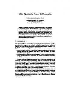
This section shows comparative simulations of ESP against other commonly used projection algorithms. Each algorithm is presented with an irredundant halfspace description of  a polytope P , (x, y) ∈ Rd × Rk | Cx + Dy ≤ b and the output of the algorithm is an  irredundant halfspace description of the projection πd (P ) = x ∈ Rd ∃y ∈ Rk (x, y) ∈ P . Four algorithms have been compared: • Fourier Elimination: This algorithm was implemented in C as described in [15]. 37

• Projection Cone: If the projection cone is defined as W , {v | vD = 0, v ≥ 0 }, then the projection is given by πd (P ) = {x | (vC)x ≤ vb, ∀v ∈ extr W }. The extreme rays of W were computed via the double description method CDD, which is implemented in C [8]. • Vertex Enumeration: In this approach, the vertices of the polytope P are enumerated, projected and then the convex hull of the projection is calculated. All computations are done via the double description method CDD [8]. • ESP: The ESP algorithm is implemented in Matlabr and all linear programs are computed via the Stanford Systems Optimization Laboratory (SOL) toolbox [12]. As we require the output to be irredundant, each inequality generated by the first two approaches is tested for redundancy by a call to a linear program. The LP code used is the Stanford Systems Optimization Laboratory (SOL) toolbox [12]. The polytopes that are used in this comparison are randomly generated, bounded by a hypersphere of radius 10 and all inequalities in their description are irredundant. Figure 11 shows the results of the simulations where the y−axis is a logarithmic scale of the time taken per facet of the projection and the x−axis is the variable ξ, which is defined in the following list. Let q be the number of halfspaces in the description of P and we define four scenarios: a.

R10 −→ R4 , q = ξ, ξ = 10, . . . , 100 This test demonstrates the complexity of the algorithms as a function of the number of halfspaces in the polytope. From (25) and recalling that an LP has linear complexity
for fixed dimension, the complexity per facet of the projection of ESP is O q 2 ; this tendency can be seen in Figure 11(a).

b.

Rξ −→ R4 , q = 3ξ, ξ = 5, . . . , 30 In this test we project to a fixed dimension while increasing the dimension of the polytope P . From (25), the complexity of ESP should increase as O(LP (k, 3k)). It is clear from Figure 11(b) that for these polytopes, ESP is capable of projecting from much higher dimensions than the other approaches. The main limitation as the dimension increases is the rapid growth of the number of facets in the projection.

c.

Rξ −→ R4 , q = 2ξ, ξ = 5, . . . , 70 P is a hypercube This scenario computes the projection of rotated hypercubes to R4 . Note that while a n−dimensional hypercube has 2n facets, it contains 2n vertices. Therefore, the projection cone and vertex enumeration approaches are ill-suited in this case. However, as can be seen from Figure 11(c), ESP can handle very high dimensions.

d.

Rξ −→ R2 , q = 3ξ, ξ = 5, . . . , 50 The final test shows the projection of randomly generated polytopes from high dimensions to R2 . The procedure described in Section 5.2.1 for the calculation of ridges in 1D makes ESP particularly suited to this task, as can be readily seen from Figure 11(d). 38

Remark 38. Note that difference in speed between ESP and the other algorithms for small problems is likely to be due in large part to the overhead involved in the implementation of ESP in Matlabr . All code presented in this report can be found online at http://www-control.eng.cam.ac.uk/~cnj22/projection.html

9

Conclusion

This paper has presented the ESP algorithm, which is a new approach for the projection of polytopes in halfspace form. The proposed algorithm requires a linear number of linear programs per output facet in order to compute the projection. If the size of the polytope is kept constant, it has been shown that the complexity becomes linear in the number of facets of the projection. The algorithm has been implemented and some comparative simulations were given in Section 8. These simulations use a sample of a few classes of polytopes and we do not claim that ESP is the fastest approach in every case. For example, there is a large class of polytopes for which the projection cone has a very small number of extreme rays or the number of vertices of the polytope is small, such as in a simplex. However, the simulations presented here demonstrate that there is a large class of polytopes for which ESP is particularly suited and is able to calculate projections of polytopes in significantly higher dimensions than existing methods. Of particular note are high dimensional polytopes that are to be projected to a low dimension, polytopes represented by a small number of inequalities and hypercubes.

10

Acknowledgements

The authors would like to thank Pascal Greider for his valuable comments early in this work. Colin Jones would like to thank the Natural Sciences and Engineering Research Council of Canada and the Princes Commonwealth Trust for their support during this work. Eric Kerrigan is a Royal Academy of Engineering Post-doctoral Research Fellow and would like to thank the Royal Academy of Engineering for supporting this research.

A

Calculation of the Affine Hull

This section presents a well known algorithm for the computation of the equality set E of a polytope P such that PE = P . The input to the algorithm is the matrix A ∈ Rq×n and the vector b ∈ Rq that defines the polytope P , {z ∈ Rn | Az ≤ b}. The output is an equality set E such that PE = P and the affine hull is given by aff P = {z | AE z = bE }.

39

3

3

10

10

Vertex Enum Projection Cone ESP Fourier Elim

2

Vertex Enum Projection Cone ESP Fourier Elim

2

10

10

1

Time (sec/facet of projection)

Time (sec/facet of projection)

10 1

10

0

10

−1

10

0

10

−1

10

−2

10

−2

10

−3

10

−4

−3

10

10

20

30

40 50 60 70 ξ (Number of facets in input polytope)

80

90

10

100

5

(a) R10 −→ R4 ; ξ = number of facets in P

10

15 20 ξ (Dimension of input polytope)

25

30

(b) Rξ −→ R4 ; 3ξ = number of facets in P

2

4

10

10

Vertex Enum Projection Cone ESP Fourier Elim

1

Vertex Enum Projection Cone ESP Fourier Elim

3

10

10

2

0

Time (sec/facet of projection)

Time (sec/facet of projection)

10

10

−1

10

−2

10

1

10

0

10

−1

10

−2

10 −3

10

−3

10

−4

10

−4

5

10

15

20

25 30 35 40 ξ (Dimension of input hypercube)

45

50

55

(c) Rξ −→ R4 ; P is a rotated hypercube

10

0

10

20

30 40 ξ (Dimension of input polytope)

50

60

(d) Rξ −→ R2 ; 3ξ = number of facets in P

Figure 11: Comparative Simulation Results for Randomly Generated Polytopes

40

70

Recall that the equality set of P consists of all constraints that are active at every point in the polytope. Therefore, if a point can be found in the polytope for which a given constraint is not active, then that constraint is clearly not in the equality set. Given a constraint i ∈ {1, . . . , q}, a point exists for which it is not active if Ai z − bi is strictly less than zero for some z. We can search for such a point by minimizing the value of Ai z − bi : J(i)? , min

Ai z − bi

z

subject to

Az ≤ b.

If J(i)? is strictly negative, then constraint i is not in the equality set. If it is positive, then the constraint is redundant and if it is equal to zero then it is in the equality set.

B

Projection of non Full-Dimensional Polytopes

If πd (P ) is not full dimensional, then P must have a non-trivial affine hull and there exists an equality set A such that PA = P . An algorithm for computing the affine hull of a polytope, and the equality set of the constraints that determine it is given in Appendix A. If A is the equality set of the affine hull, then from Proposition 21 we can write the projection πd (P ) as πd (P ) = {x ∈ Rn | ∃y, F x = f, Cx + Dy ≤ b } , where F , N DA T


T

CA and f , N DA T


T

(26)

bA . We now form a polytope Pe that satisfies

the assumption that its projection is full-dimensional and from which we can recover the projection πd (P ). The equation F x = f can be equivalently written as x = N(F )e x + F † f , for x e ∈ Rdim πd (P ) , where we note that dim πd (P ) = n − rank F . The polytope πd (P ) then becomes n πd (P ) = x ∈ Rn n = x ∈ Rn

o † e ∃y, x = N(F )e x + F f, (e x , y) ∈ P  o x + F † f, x e ∈ πdim πd (P ) Pe x = N(F )e

where n o Pe , (e x, y) CN(F )e x + Dy ≤ b − CF † f .

41

  We now show that Pe satisfies the assumption that πdim πd (P ) Pe is full-dimensional.   πdim πd (P ) aff Pe

n o = πdim πd (P ) x e ∃y, CA N(F )e x + DA y = bA − CA F † f n o
T
T  = x e N DA T CA N(F )e bA − C A F † f x = N DA T = Rdim πd (P )

(27)


T where (27) follows because F is defined as N DA T CA . Once the projection of Pe is computed using ESP, an expression is needed   to recover T πd (P ). x e can be written as a function of x as N(F ) x = x e. If πdim π (P ) Pe is given by d

{e x | Ge x ≤ g} then n o πd (P ) = x x = N(F )e x + F † f, Ge x≤g n o = x F x = f, GN(F )T x ≤ g .

C

Projection of Polytopes that do not Contain the Origin

In this section we consider a polytope P that does not contain the origin in its interior. The solution presented here is to compute a strictly interior point (x0 , y0 ) and then translate the polytope such that this point gets mapped to the origin. After running ESP on the translated polytope, the projection is then translated back by −x0 to restore the origin placement. The following linear program will compute an interior point of polytope P whose equality set is A: (x0 , y0 ) , argmin

τ

(τ,x,y)

subject to

CAc x + DAc y ≤ bAc + τ

(28)

CA x + DA y = bA b TranslatingP by (x ≤ b + Cx0 +oDy0 }. If the projecn0 , y 0 ) gives oP , {(x, y) | Cxn+ Dy b ≤ gb , then πd (P ) = x Gx b ≤ gb − Gx b 0 . tion of Pb is πd Pb = x Gx

References [1] Nina Amenta and G¨ unter M. Ziegler. Shadows and slices of polytopes. In Proceedings of the twelfth annual symposium on computational geometry, pages 10–19. ACM Press, 1996.

42

[2] D. Avis. lrs: A revised implementation of the reverse search vertex enumeration algorithm. In G. Kalai and G.M. Ziegler, editors, Polytopes — Combinatorics and Computation, pages 177–198. Birkhauser-Verlag, 2000. [3] Egon Balas. Projection with a minimum system of inequalities. Computational Optimization and Applications, 10:189–193, 1998. [4] Egon Balas and Maarten Oosten. On the dimension of projected polyhedra. Discrete Applied Mathematics, 87:1–9, 1998. [5] Michel L. Balinski. On the graph structure of convex polyhedra in n-space. Pacific Journal of Math, 95(11):431–434, 1961. [6] F. Blanchini. Set invariance in control. Automatica, 35(11):1747–1767, 1999. Survey Paper. [7] Herbert Edelsbrunner and Ernst Peter M¨ ucke. Simulation of simplicity: A technique to cope with degenerate cases in geometric algorithms. ACM Transactions on Graphics, 9(1):66–104, 1990. [8] K. Fukuda and A. Prodon. Double description method revisited. In M. Deza, R. Euler, and I. Manoussakis, editors, Combinatorics and Computer Science, volume 1120 of Lecture Notes in Computer Science, pages 91–111. Springer-Verlag, 1996. Postscript file available from ftp://ftp.ifor.math.ethz.ch/pub/fukuda/reports/ddrev960315.ps.gz. [9] Komei Fukuda, Thomas M. Liebling, and Christine L¨ utolf. Extended convex hull. In 12th Canadian Conference on Computational Geometry, pages 57–64, July 2000. [10] Joxan Jaffar, Michael J. Maher, Peter J. Stuckey, and Roland H. C. Yap. Projecting clp(R) constraints. New Generation Computing, 11(3,4):449–469, 1993. [11] Eric Kerrigan. Robust Constraint Satisfaction: Invariant Sets and Predictive Control. PhD thesis, University of Cambridge, 2000. [12] Walter Murray and Michael Saunders.

Systems Optimization Laboratory (SOL).

http://www.sbsi-sol-optimize.com. [13] Jean Ponce, Steve Sullivan, Attawith Sudsang, Jean-Daniel Boissonnat, and Jean-Pierre Merlet. On computing four-finger equilibrium and force-closure grasps of polyhedral objects. International Journal of Robotics Research, February 1995. [14] R. Tyrrell Rockafellar. Convex Analysis. Princeton University Press, 1970. [15] Vijay Saraswat and Pascal Van Hentenryck, editors. Principles and Practice of Constraint Programming, chapter 14, pages 245–268. The MIT Press, 1995. 43

ˇ [16] S.N. Cernikov. Contraction of finite systems of linear inequalities (in russian). Doklady Akademiia Nauk SSSR, 152(5):1075–1078, 1963. (English translation in Societ Mathematics Doklady, Vol. 4, No. 5 (1963), pp.1520-1524). [17] R. Vidal, S. Schaffert, J. Lygeros, and S. Sastry. Hybrid Systems: Computation and Control, volume 1790 of Lecture Notes in Computer Science, chapter Controlled Invariance of Discrete Time Systems, pages 437–450. Springer Verlag, 2000. [18] Roger Webster. Convexity. Oxford University Press, 1994. [19] G¨ unter M. Ziegler. Lectures on Polytopes. Springer-Verlag, New York, first edition, 1995.

44