3482
JOURNAL OF CLIMATE
VOLUME 26
CORRESPONDENCE Comments on ‘‘Erroneous Model Field Representations in Multiple Pseudoproxy Studies: Corrections and Implications’’ SCOTT D. RUTHERFORD Department of Environmental Science, Roger Williams University, Bristol, Rhode Island
MICHAEL E. MANN Department of Meteorology, and Earth and Environmental Systems Institute, The Pennsylvania State University, University Park, Pennsylvania
EUGENE WAHL National Climatic Data Center, National Oceanic and Atmospheric Administration, Boulder, Colorado
CASPAR AMMANN Climate Global Dynamics Division, National Center for Atmospheric Research, Boulder, Colorado (Manuscript received 26 January 2012, in final form 5 October 2012) ABSTRACT Smerdon et al. report two errors in the climate model grid data used in previous pseudoproxy-based climate reconstruction experiments that do not impact the main conclusions of those works. The errors did not occur in subsequent works and therefore have no impact on the results presented therein. Results presented here for the Climate System Model (CSM) using multiple pseudoproxy noise realizations show that the quantitative differences between the incorrect and corrected results are within the expected variability of the noise realizations. It should also be made clear that the climate reconstruction method used in Smerdon et al. to illustrate the nature of the errors, the Regularized Expectation Maximization method with Ridge Regression (RegEM-Ridge), is known to produce climate reconstructions with considerable variance loss and has been superseded by RegEM-TTLS (TTLS indicates truncated total least squares).
Smerdon et al. (2010) describe two technical errors in the model grid data used in Mann et al. (2005, 2007a). They are correct in the discovery of these errors. We wish to confirm that the errors did not occur in subsequent publications and that the main conclusions of Mann et al. (2007a), which supersedes Mann et al. (2005), are not impacted. First, Mann et al. (2005) used the Regularized Expectation Maximization method with Ridge Regression (RegEM-Ridge) as a regularization method. RegEMRidge has been shown to suffer from a loss of variance Corresponding author address: Scott Rutherford, Department of Environmental Science, Roger Williams University, Bristol, RI 02809. E-mail:
[email protected] DOI: 10.1175/JCLI-D-12-00065.1 Ó 2013 American Meteorological Society
when reconstructing the hemispheric mean (F. Zwiers and T. Lee 2006, personal communication; Mann et al. 2007a,b; Smerdon and Kaplan 2007; see also Lee et al. 2008), which is not the case with RegEM-TTLS (TTLS stands for truncated total least squares, used for regularization). This led Mann et al. (2007a) and others (e.g., Riedwyl et al. 2009) to abandon RegEM-Ridge in favor of the TTLS implementation of RegEM. This being the case, we will confine our comments to Mann et al. (2007a). However, it is important that the reader recognize that Smerdon et al. (2010) used RegEM-Ridge and that the results shown in their Fig. 5a show the expected variance loss of a RegEM-Ridge reconstruction, whereas RegEMTTLS reconstructs the target series with little to no variance loss (Fig. 1; Table 1).
15 MAY 2013
CORRESPONDENCE
3483
FIG. 1. Corrected Northern Hemisphere mean reconstructions for both the (a) GKSS and (b) CSM (Rutherford et al. 2010) model fields, respectively (20-yr smoothed). Note that RegEM-TTLS faithfully reconstructs the target series with little to no variance loss, especially at the important multidecadal and longer time scales. To facilitate comparison, series for both models are calculated over all grid boxes between 08 and 708N. The results shown are for 104 white-noise pseudoproxies with a signal-to-noise ratio of 0.4 and a 1900–80 calibration period.
Smerdon et al. (2010) address two issues with GCM field data used in Mann et al. (2007a). The first relates to the GKSS model field. In a previous comment/reply sequence (Smerdon et al. 2008; Rutherford et al. 2008), the method used to interpolate the GKSS model field to a resolution commensurate with the instrumental record was changed from that of Mann et al. (2007a) to address an issue with the hemispheric mean. Unbeknownst to us at the time, the changes made to implement the revised interpolation scheme must also have corrected the issue of incorrect longitude orientation of the model field and subsequent pseudoproxy locations raised in Smerdon et al. (2010), as that issue does not exist in the data used in Rutherford et al. (2008). Thus, issues with the GKSS field identified by Smerdon et al. existed in Mann et al. (2007a) but not in subsequent works, including Rutherford et al. 2008. The second issue relates to the incorrect longitudes for the interpolated Climate System Model (CSM) field. The authors have correctly identified an error that occurred in the process of converting the CSM field into a format consistent with the available instrumental data
so that an instrumental-data mask could be applied. As Smerdon et al. point out, this error does not impact the qualitative conclusions drawn from the results and described in Mann et al. 2007a (cf. Fig. 1). The global field was still reasonably sampled with the correct latitudinal distribution of pseudoproxy locations. Comparing the CSM results using the incorrect Mann et al. (1998) proxy locations and the corrected locations with the full field (Table 1) indicates that the method produces similar results using different proxy networks as long as the field is adequately sampled. As an additional example, replicate analyses using the full model field to 708N, corrected longitude values, and 30 different pseudoproxy realizations with 104 pseudoproxies coupled with a 1900–80 calibration period and a signal-to-noise ratio of 0.4 produce a NH mean reduction of error (RE) (Cook et al. 1994) score of 0.93 6 0.06 (mean 6 two standard deviations), a Northern Hemisphere (NH) mean coefficient of efficiency (CE) (Cook et al. 1994) score of 0.45 6 0.25, a mean multivariate RE score of 0.33 6 0.08, and a CE score of 20.07 6 0.14. These scores are consistent with the scores reported in
3484
JOURNAL OF CLIMATE
TABLE 1. Comparison of verification scores for incorrect and correct (boldface) reconstructions (shown in Fig. 1) for both the GKSS and CSM fields. To facilitate comparison, corrected verification scores for both models are calculated over all grid boxes between 08 and 708N. Results are shown for white noise, signal-tonoise ratio of 0.4, the 1900–80 calibration period, the 850–1855 verification period for CSM, and the 1000–1855 verification period for GKSS. Additional correct results and discussion can be found in Mann et al. (2009, see their supplemental Table S2) and Rutherford et al. (2010). The ‘‘NH mean’’ scores are for the Northern Hemisphere mean series and ‘‘Multivariate’’ indicates spatiotemporal scores calculated on all grid boxes over the verification period. Data are from Mann et al. 2007a (rows 1 and 3) and this study (rows 2 and 4); RE is reduction of error and CE is coefficient of efficiency (Cook et al. 1994).
Model
NH mean RE
NH mean CE
Multivariate RE
Multivariate CE
GKSS GKSS CSM CSM
0.94 0.96 0.95 0.96
0.93 0.84 0.67 0.70
0.68 0.32 0.36 0.35
0.46 20.09 0.04 20.04
Mann et al. (2007a) (see their supplementary Fig. 5) for multiple noise realizations (average scores for three replicates of 0.93, 0.54, 0.34, and 0.01, respectively). Smerdon et al. further note that the Ni~ no-3 results shown in Mann et al. (2007a) are incorrect as they do not represent the Ni~ no-3 region. Since Mann et al. (2007a), an extensive evaluation of RegEM-TTLS in tropical Pacific sea surface temperature (SST) reconstructions has been conducted using updated proxy networks, calibration periods, and methods (for both pseudoproxy and real-proxy contexts) (Emile-Geay et al. 2013a,b). It should also be made clear to the reader that later publications, Mann et al. (2009; see their supplementary Table S2), Rutherford et al. (2010), and Schmidt et al. (2011), which used the CSM field, do not suffer from the longitude problem associated with conversion to a format consistent with the available instrumental data because there was no attempt to apply such a data mask. The results of these subsequent works show the general results and conclusions of Mann et al. (2007a) to be robust (cf. Table 1) and use updated calibration intervals and/or revised methods (Mann et al. 2009; Rutherford et al. 2010). Finally, the discovery of these errors illustrates the importance of mapping/plotting each stage of data conversions to identify errors when they occur. By the time one plots the resulting mean series, errors in the regridding are hidden. Furthermore, even a map of the inverted CSM longitudes for a particular year looks reasonable
VOLUME 26
and illustrates the importance of independent checks on the actual code used. REFERENCES Cook, E. R., K. R. Briffa, and P. D. Jones, 1994: Spatial regression methods in dendroclimatology: A review and comparison of two techniques. Int. J. Climatol., 14, 379–402. Emile-Geay, J., K. M. Cobb, M. E. Mann, and A. Wittenberg, 2013a: Estimating central equatorial Pacific SST variability over the past millennium. Part I: Methodology and validation. J. Climate, 26, 2302–2328. ——, ——, ——, and ——, 2013b: Estimating central equatorial Pacific SST variability over the past millennium. Part II: Reconstructions and implications. J. Climate, 26, 2329–2352. Lee, T. C. K., F. W. Zwiers, and M. Tsao, 2008: Evaluation of proxy-based millennial reconstruction methods. Climate Dyn., 31, 263–281, doi:10.1007/s00382-007-0351-9. Mann, M. E., R. S. Bradley, and M. K. Hughes, 1998: Global-scale temperature patterns and climate forcing over the past six centuries. Nature, 392, 779–787. ——, S. Rutherford, E. Wahl, and C. Ammann, 2005: Testing the fidelity of methods used in proxy-based reconstructions of past climate. J. Climate, 18, 4097–4107. ——, ——, ——, and ——, 2007a: Robustness of proxy-based climate field reconstruction methods. J. Geophys. Res., 112, D12109, doi:10.1029/2006JD008272. ——, ——, ——, and ——, 2007b: Reply. J. Climate, 20, 5671–5674. ——, and Coauthors, 2009: Global signatures and dynamical origins of the Little Ice Age and Medieval Climate Anomaly. Science, 326, 1256–1260. Riedwyl, N., M. Ku¨ttel, J. Luterbacher, and H. Wanner, 2009: Comparison of climate field reconstruction techniques: Application to Europe. Climate Dyn., 32, 381–395, doi:10.1007/ s00382-008-0395-5. Rutherford, S., M. E. Mann, E. Wahl, and C. Ammann, 2008: Reply to comment by Jason E. Smerdon et al. on ‘‘Robustness of proxy-based climate field reconstruction methods.’’ J. Geophys. Res., 113, D18107, doi:10.1029/2008JD009964. ——, ——, C. M. Ammann, and E. R. Wahl, 2010: Comments on ‘‘A surrogate ensemble study of climate reconstruction methods: Stochasticity and robustness.’’ J. Climate, 23, 2832– 2838. Schmidt, G. A., M. E. Mann, and S. D. Rutherford, 2011: Discussion of: ‘‘A statistical analysis of multiple temperature proxies: Are reconstructions of surface temperatures over the last 1000 years reliable?’’ Ann. Appl. Stat., 5, 65–70. Smerdon, J. E., and A. Kaplan, 2007: Comments on ‘‘Testing the fidelity of methods used in proxy-based reconstructions of past climate’’: The role of the standardization interval. J. Climate, 20, 5666–5670. ——, J. F. Gonza´lez-Rouco, and E. Zorita, 2008: Comment on ‘‘Robustness of proxy-based climate field reconstruction methods’’ by Michael E. Mann et al. J. Geophys. Res., 113, D18106, doi:10.1029/2007JD009542. ——, A. Kaplan, and D. E. Amrhein, 2010: Erroneous model field representations in multiple pseudoproxy studies: Corrections and implications. J. Climate, 23, 5548–5554.