Error Minimising Pipeline for Hi-Fidelity, Scalable Geospatial Simulation Chris Thorne School of Computer Science and Software Engineering The University of Western Australia
[email protected]
Abstract The geospatial category of simulations is used to show how origin centric techniques can solve a number of accuracy related problems common to 3D computer graphics applications. Previous work identified how poor understanding of floating point related issues lead to performance, architectural and accuracy problems. This paper extends that work by including time error minimisation, lazy evaluation and progressively refined fidelity and looks at performance trade-offs. The application of these techniques to a geospatial simulation pipeline is described in order to provide more concrete guidance on how to use them.
I. Introduction Geospatial simulations are increasingly important in modern times, providing rich, 3D location-based content and behavior for a wide range of purposes. They have dramatically risen in popularity and use since the inception of Google Earth[1], NASA’s WorldWind[2] and Microsoft’s Virtual Earth[3] which have become the focus of information sharing on a massive scale. Despite increasing power and quality of modern computers, the fidelity of simulations does not achieve the photoreal dream of Gibson’s cyberspace worlds [4] due to floating point accuracy related problems, such as spatial jitter[5], z buffer clipping, and inaccurate rendering. The causes lie in the nature of the simulation environment, how we currently navigate through simulations and the level of understanding of floating point and accuracy problems. Modern simulations are generally performed in a 4D floating point virtual space of (x,y,z) coordinates and time. Floating point is used extensively in simulation compu-
tation whether it be for industry, science, engineering or entertainment. These simulations also execute in a system environment with a narrowing precision bottleneck as one goes from input through to output. For performance and space reasons, graphics pipelines use floating point values with precision no greater than single precision floating point, and often less [6,7], for coordinates. However, geospatial applications need greater precision and must maintain object geographic position in double precision [8]. Thus, the simulation may use double precision but as processing moves to the graphics output it will be reduced to single precision in the graphics software and then even to lower precision in the graphics hardware. Two key factors combine to cause floating point accuracy related problems in simulations: a spatial position dependent error, the Spatial Epsilon Error (SEE) [9], that increases with coordinate size, and conventional originrelative viewpoint navigation. For convenience, SEE will be referred to as spatial error in the remainder of this paper. The error is magnified by calculation relative error and the decreasing floating point precision of variables as they are funneled down the pipeline bottleneck. Developers of simulations have not fully understood these floating point accuracy issues nor how best to manage them and typically underestimate the size of error. Consequently, they have no well proven and accepted way of designing their applications to prevent such problems and attain the highest accuracy and scalability. This paper provides a generic solution applicable to all simulation that uses floating point modelling and calculation. An Origin Centric (OC) approach: the Floating Origin Architecture (FOA), was introduced in [5] to improve accuracy, avoid spatially dependent problems and reduce calculation error by reducing spatial error. Rendering inaccuracies caused by spatially dependent error are described in [9]. This paper expands on those works and goes into more detail on how and where to apply origin centric
methods with respect to the stages of a simulation pipeline model. The geospatial category of simulations (geosim) was chosen because their large scale exascerbates the extent of floating point related error. A distributed, rather than standalone model was also chosen because of the growing importance of distributed geospatial applications, such as Web Map Server (WMS) compatible applications (e.g. GeoServer), Google Earth, WorldWind and Virtual Earth. Additionally, it is only practical to include the network because data that may be required at any one time can come from any part of a volume so large that it cannot be stored or downloaded to a client machine entirely. This paper looks at the simulation pipeline architecture of geosims from input to final output. Apart from the Author’s previous work [5,9,10], there has been no published research on origin centric techniques. The closest was the work on GeoVRML [11] and Terravision [12]. Generally, practitioners and researchers have taken ad-hoc approaches to solving accuracy related problems. Research to date has resulted in the implementation of parts of the Floating Origin (FO) framework on the planet-earth application [10]. However, implementation could not go far enough because changes to the client graphics architecture were required and the client graphics display software used was closed source. The next step will be to modify an open source graphics client to implement the methods detailed here.
II. General structure of a distributed simulation pipeline The general structure of a simulation pipeline is illustrated in Figure 1 which shows the flow of information from input to output. Feedback in the other direction from any stage is also possible. The generic components of a simulation pipeline are data acquisition, modelling, implementation, visualisation and other forms of output such as reports/results data and analysis. This paper is only concerned with interactive video output but the results can also apply to other forms of output, such as printed reports or numerical tables. The visualisation stage is often referred to as a graphics pipeline [13], as is depicted in Figure 2, which shows graphical model as input to the graphical scene. The scene is animated, usually in response to user interaction, through a number of operations such as a rotation, translation and view transformations and is then rendered from the user’s point of view. Many other graphical algorithms are used: for example, clipping, viewport transformation, shading, and rasterization are just a few. Figure 3 shows a distributed simulation pipeline where the arrows are made bidirectional to show feedback. In
2
the Figure, there is a macro level subdivision of the pipeline into Object System (OS) and Display System (DS), signified by the solid black boxes, in keeping with the floating origin architecture described in [5]. The OS maintains the whole simulation model and keeps track of object position and state. Objects are passed down the pipeline to the DS which renders the user’s view into the simulation. Positions of objects in the OS are commonly described as World Coordinates (WC). The DS is mainly concerned with graphics output and this is also where one may consider the graphics pipeline to be. However, although the graphics pipeline is concerned mainly with the final output stage of simulation, in Figure 3, it has been extended back into the simulation pipeline because the graphical models are part of the input stage of both pipelines. Also, in a modern distributed graphical application, it is possible for some graphical information to be generated by peer clients or servers and transmitted across the network. The coordinates used in the later part of the graphics pipeline are normally cartesian: (x,y,z) floating point tuples. Graphical models are represented using a local coordinate system. Each model can be described in a number of different ways, such as parametrically [14], procedurally [15] or as a triangulated set of vertices [16] defining polygons. In most cases, the models end up being converted to (x,y,z) vertices representing simple polygons, such as triangles, so objects will be treated as vertex sets for the remainder of this paper. An object’s vertices are given in its local coordinate system. To place the object correctly in relation to other parts of a scene, the world coordinate position of the object is added to its local vertex coordinates at some stage in the pipeline. The vertices, along with other properties, then describe the final object to be rendered. Simulation needs to be customised to the subject being simulated and details of the pipeline will change accordingly. Therefore, to provide a concrete example of applying OC techniques, the geospatial simulation pipeline is used in the remaining discussion.
III. A distributed pipeline
geospatial
simulation
Figure 4 shows key elements of a geosim pipeline are cartographic input, geospatial models, calculations and geospatial projections. In the modelling stage, there will be a mathematical world model, such as ellipsoidal [17], in addition to graphical models of world and objects. The world coordinates of a geospatial application are normally represented in an accepted goespatial reference system, such as geographic (latitude, longitude, height). Others are cartesian (x,y and z values for orthogonally
aligned axes), Military Grid Reference System (MGRS), Australian Map Grid (AMG), polar coordinates, and many more. For simplicity, geographic coordinates will be assumed for the rest of this paper. Since time is also a positional parameter (we measure things in relation to their position in time), the OC spatial error minimisation approach can also be applied to time error minimisation. The following section puts the OC approach into the context of geospatial simulation and extends the earlier techniques with time error minimisation, lazy evaluation [18] and progressively refined fidelity (PRF).
IV. Error minimising distributed geospatial simulation pipeline A. Entry to pipeline The first place to minimise error is in the collection and storage of cartographic input to the pipeline. As described earlier, the position of an object is eventually added to the object’s local vertex coordinates to correctly position it relative to everything else. This step could be performed at the very beginning: when models are first input into the pipeline. That is, for a static object, such as a house, we could add the position coordinate to each of the object’s vertex coordinates and it would thereafter be correctly positioned. The problem with this approach is that it can result in the object coordinates becoming very large, causing a large increase in error. Once the addition is performed, the higher accuracy of the smaller local vertex coordinates is lost. Note that this description applies to static objects only because moving object local coordinates are naturally kept separate from their object position. To illustrate, consider a house less than 20m radius. Its geographic position, after conversion to cartesian, is (1,2000,000, 2,400,000, 1,000,000). This is not an unusually large coordinate value because the earth has a radius of about 6,400,000m and even geospatial coordinate systems which break the world into smaller local regions, such as Australian Map Grid, have coordinates that reach 7 decimal digits. Now, 7 decimal digits equates to approximately 20 binary digits to represent the value (220 = 1, 048, 576). Given that accuracy falls off with increasing coordinate size, adding a 7 digit position coordinate to each vertex coordinate would result in a loss of up to 20 bits of accuracy. A real world example of this kind of unnecessary accuracy loss was found in 3D scan data collected from SiroVision [19] scans. Therefore, one should delay adding the geographic position to object vertex coordinates until it is close to the origin, where only a small offset will be added.
B. Applying the origin centric approach
3
The origin centric approach exploits the facts that floating point numbers have their highest accuracy near the origin and the place where most accuracy is needed is where observations are made: the viewpoints from which images of the simulation are rendered. Putting the two together leads to the approach where the scene origin “floats” with the viewpoint as the user navigates the virtual world. During navigation, the viewpoint is maintained the origin in DS coordinate space as the user navigates. Objects are moved in reverse via a top level reverse World Transform (WT) which sits above scene objects. Whenever the graphics pipeline fetches object position, the position is combined with the top level translation. The effect is to translate objects in reverse as the user navigates, giving the same relative motion between viewpoint and objects as in conventional navigation. This technique minimises the size of coordinate values the closer they are to the viewpoint thereby raising their accuracy to a high level. Other techniques are also required to make OC work well, some of which were described in [5], such as modified viewpoint handling, collision detection and new techniques are discussed in this paper. The small valued, accurate, coordinates in turn lead to more accurate rendering, motion, calculation and interaction. This approach contrasts to the conventional originrelative navigation of most modern graphics applications, where coordinates can attain arbitrarily large values with correspondingly large SE error. Returning to the house example, since most visualisation of the object will be performed from a position close to it, say 100m to 1km away, there will almost never be a time when the full 7 digit geographic coordinates need to be added to its vertex coordinates. Instead, a floating origin subtraction (Figure 5) is performed: the observer’s WC position is subtracted from the house’s WC, to place it correctly in the environment (because the observer’s position is maintained at (0,0,0) in the DS). After the subtraction, only the small resulting difference is added to the object’s vertex coordinates to place it in the environment. Hence, most of the 20 bit precision loss in vertex coordinates is bypassed entirely. Figure 5 shows the progression of object coordinates and vertices through the pipeline. Note the stages where the floating origin subtraction is made, the addition of object position to vertex coordinates and conversion from double to single precision. The OS provides updates of user and moving object positions periodically to the server. The best place to perform such a subtraction in the pipeline is just prior to conversion from double precision values to single precision values (see Figure 5).
It should be understood that the FO subtraction does not of itself increase accuracy in the values of coordinate variables because the precision is the same before and after the subtraction. FO subtraction only significantly improves accuracy when used prior to a step down in precision as described above. However, it does minimise the resulting values and when they are then used as input to calculations this reduces relative error propagation because more precision is available to the smaller floating point mantissas [20] in every step of the calculation. Evidence that this, combined with an origin centered navigation, can improve the fidelity and scalability of an entirely single precision system was provided by early versions of the planet-earth project. These versions were pure VRML2.0, running on a client with no double precision server support. VRML2.0 only contains single precision floating point fields and yet the project was able to scale its planet simulation up from a non floating origin size limit of approximately 100,000m to support a continuous model larger than the size of the earth.
C. Time accuracy Time is maintained at high precision and is often stored as an integer, such as in the Linux [21] operating system and the DIS [22] simulation standard but can also be stored as a floating point value, e.g. in VRML [23] or X3D [24]. Whether it is stored as integer or floating point, when performing floating point calculations, all parameters are usually converted to floating point prior to performing the calculations. Therefore, for the matters addressed in this paper, time will be treated as a floating point positional value that can be subject to OC treatment. To apply OC to time, it must be 0 for the observer in the DS but we still need simulation time to advance for the observer relative to the virtual environment. Hence, time for objects in the DS is decremented as simulation time, held in the OS, advances. Thus, relative to everything else, time for the user still advances. The difference between the user’s frame of reference in the DS and its simulation frame of reference in the OS is maintained by OS which tracks the real simulation time for user viewpoints and objects alike. This approach moves us away from an arbitrary DS time origin of conventional simulation, where the amount of time error introduced into calculations is correspondingly arbitrary.
D. Lazy evaluation A basic principle behind the error minimising pipeline is lazy evaluation. Lazy evaluation is “a technique that attempts to delay computation of expressions until the results of the computation are known to be needed”
4
[18]. Here we apply lazy evaluation in conjunction with coordinate size minimisation to increase the accuracy of calculations, such as geographic projections. The house example demonstrated lazy evaluation: by delaying the geo-locating of the house until needed, we were able to bypass most of the loss of accuracy. Another example of applying lazy evaluation with FO subtraction is when using Level of Detail (LOD) [16]. LOD is a common geostpatial operation where the detail of terrain and other objects is increased as the viewpoint moves closer to the object. Consider the viewpoint moving towards a place where an object is located in the OS. An object only needs to be placed in the display environment if it is to be visible. At some distance, the object will be visible at low detail. At this time, a geographic projection converts its WC position into cartesian coordinates at double precision, a floating origin subtraction is performed and the resulting coordinates converted to single precision. The object is then placed in the DS environment and becomes visible. As the viewpoint moves closer, the object is dynamically replaced with a more detailed version. In step with this increase in detail, we now also repeat the same positioning operations as before to place it with even higher accuracy, because the object is now closer to the origin. As the observer moves closer, the object is dynamically replaced with a progressively finer detailed version positioned with a progressively refined fidelity. Progressively refined fidelity is an aspect of OC that can be applied to all calculations in a simulation as the point of observation moves closer to the point at which the calculation is performed. It can therefore lead to improvements in, for example, the motion of vehicles, rendering and interaction.
E. Origin centric transforms and performance In [5], performance benefits were described whereby the FO architecture allowed for a continuous world without artificial boundaries and the overheads that such boundaries invoked. This sections looks at other potential performance trade-offs when using FO. At the core of interactive computer graphics is a matrix operation, called the transformation matrix [14]. This matrix is designed to perform 3 operations on object vertices: translation, scaling and rotation and is used to move objects or can be used similarly to manipulate the view vector. Another essential type of matrix is the projection matrix. There is a point in the graphics pipeline where the transformation matrix is used to transform vertices of objects or the view. In the FO system, the translation part for the view is no longer applied at the same place, but rotation and scaling remain unchanged. The translation
resulting from user navigation is applied to the world transform instead, as previously described. One must weigh the benefits of FO against potential performance losses in implementing parts of the architecture. A possible performance overhead is when using the world transform to perform the FO subtraction on object positions. When the position of an object is fetched to be used in the pipeline, the world transform translation must be applied. This adds the slight additional overhead of three subtractions for every object position fetched. On the other hand, a potential performance benefit lies in a simplification of the remaining rotation and scaling operations. Rotation involves trigonometric operations that rotate a coordinate about another point in space. Scaling shrinks or enlarges the coordinate values and also requires a center point about which the scaling occurs. Rotation and scaling about an arbitrary point in space require additional translation operations. For example, there are three main steps to a rotation operation: a. translate the coordinate by the inverse of the center of rotation, b. rotate the coordinate, and c. translate the result back. If the center of rotation is (0,0,0) then the first and third operations are not performed. The same applies to scaling. To be specific, in the graphics pipeline, rotations, scaling and translations are performed in a combined matrix. For example, from 2D rotation examples in [14], rotation about the origin is performed by the transformation matrix: cosθ sinθ 0 −sinθ cosθ 0 0 0 1 whereas rotation about an arbitrary point is a more complex matrix: cosθ sinθ 0 −sinθ cosθ 0 x1(1 − cosθ) + y1sinθ (y1(1 − cosθ) − x1sinθ 1 The third row shows the additional operations required to rotate about an arbitrary point. Extending to 3 dimensions adds more operations, but a detailed exposition is beyond the scope of this paper so a single example from [16] is given. In this example, a 3D rotation matrix for a rotation about a point (x,y,z), with rotation axis parallel to thez axis is given in [16] as: cosθ − sinθ 0 − x.cosθ + y.sinθ + z sinθ cosθ 0 − x.sinθ − y.cosθ + y 0 0 1 0 0 0 0 1 It can be seen from the third column above that rotation about a 3D point, when aligned to an axis, requires additional calculations (6 additions, 4 multiplications and 4 trigonometric operations). Rotating about an arbitrary 3D point and axis is equivalent to three of the above matrices,
5
requiring a total of 18 additions, 12 multiplications and 12 trigonometric operations. These operations are used to construct the composite transform matrix, yielding a single value in each of the (0,4) and (1,4) positions. The latter two values are part of what each vertex in the scene is multiplied by. These extra operations are not required when the rotation is about the origin. How much difference the extra construction operations and the extra two terms per vertex multiply make will depend on the implementation. If the transform is performed in software, there will likely be a measurable difference, if it is performed in hardware Graphics Processing Unit (GPU), with fixed wiring and timing for transforms, there may be no difference. When rotating objects about a viewpoint, since the FO approach keeps the viewpoint at the origin, it implies the rotation will save the overhead shown above. Rotating about the viewpoint, or rotating the viewpoint itself, is a frequent operation when navigating a 3D world and saving on the additional operations per rotation will lead to an improvement in performance. Note, conceptually, an implementer may think it is more efficient to rotate/move the view vector(s) instead but all advice on this in forums has indicated that, in practice, there generally will be no performance difference between rotating viewpoint or rotating objects about the viewpoint. There are other situations, where such rotation performance benefits could come into play. Many military geospatial simulations and also games have a commonly used mode where the viewpoint is offset from a Center of Interest (COI). In the case of a military system, the COI would be a moving vehicle, as seen from a displaced viewpoint. As the vehicle “moves” it remains at the center of the screen and scene objects move in reverse, similar to FO. In a computer game, the COI would be the user’s avatar, with the viewpoint displaced to see the avatar in relation to the rest of the scene. The viewpoint is tied by an elastic tether to the avatar and, although it can be adjusted independently, moves with it. In the military system example, the viewpoint is only tethered to look at the vehicle at the center of the screen. These COI systems could utilise a FO method where the origin floats with the COI and viewpoint is now tethered at a distance from the origin. Note, in this case, the axis of rotation/pivot of the camera is not tied to the axis of rotation of the avatar in games. With this tethered FO approach, the performance savings described for rotations about the origin can apply, because they are independent of the view vector manipulation. The performance saving from rotating objects about the origin would be proportional to the complexity of the scene (number of objects and vertices) being rotated. Some calculation savings also apply to scaling for similar reasons. No definitive statement will be possible as to over-
all performance gains or losses because there is both a high complexity and huge variation in the way modern graphics software and hardware are implemented. There is some standardisation via the Shader 2.0 [7], Directx [27] and openGL [28] specifications but these do not prevent vast differences in implementations. Therefore, extensive implementation tests are required to evaluate the performance trade-offs. Future work will focus on two reference implementations to evaluate the complete FO architecture, including the tethered version. As there are modifications required to the graphics pipeline, some open source graphics engines will be selected. One implementation will be selected from a C++ open source graphics engine and one from a java open source engine. At the present time, no specific candidates have been selected but possibilities for the C++ implementation are: Flux [29], Ogre3D [30] or derivatives, OSG [31], or NASA’s WorldWind; and for the Java implementation xj3d [32].
V. Conclusion This paper extends earlier work designed to improve the accuracy and scalability of 3D computer simulation by describing additional techniques and implementation detail. It builds on an earlier foundation of good floating point knowledge applied to graphics and moves away from ad-hoc approaches with arbitrary fidelity to one of consistent high fidelity. When numerical computation was standardised on IEEE floating point it yielded great cost and simplification benefits for portable numerical software [33]. Standardising on an origin centric design may help achieve similar benefits for accurate numerical simulation. A geospatial simulation pipeline was used to show how and where to apply origin centric techniques to coordinate and even time variables. By maintaining the viewpoint at (or tethered to) the origin in simulation space and time, a simulation can be as accurate as the precision of the display system and calculations allow. Potential performance benefits afforded by this approach have to be balanced against other architectural changes in the simulation pipeline to support the complete origin centric approach and will be evaluated in future reference implementations. In summary, the origin centric approach respects the decreasing precision bottleneck, works in harmony with the nature of computer simulation floating point spaces and converts the nonuniform resolution weakness of these spaces into a strength by ensuring higher, optimal accuracy and scalability.
Acknowledgment The author would like to thank Associate Professor Amitava Datta for his continued support and supervision
6
and the Western Australian Premier’s Collaborative Research Program for providing funding for my research.
References [1] [2] [3] [4] [5]
[6] [7] [8] [9]
[10] [11]
[12] [13] [14] [15] [16] [17]
[18] [19] [20] [21] [22] [23] [24] [25] [26] [27] [28] [29] [30] [31] [32] [33]
http://earth.google.com/ http://worldwind.arc.nasa.gov/ http://local.live.com/ Gibson, W. F., “Burning Chrome”, published in Omni 1982, by Omni, 1982. Thorne, C., “Using a Floating Origin to Improve Fidelity and Performance of Large, Distributed Virtual Worlds”, in Proceedings of the International Conference on Cyberworlds, Nanyang Technical University, Singapore, 23-25 November, 2005, pp 263-270. Carmack, J., Carmack’s .plan files blog, 29/1/03, http://doomed.com/blog/category/doom-ed/john-carmack/, 2003. “Pixel Shader 2.0 precision”, http://www.digit-life.com/articles2/psprecision. “GeoVRML 1.1 Specification”, http://www.geovrml.org/1.1/doc/concepts.html, SRI International, 2002. Thorne, C., “Effect of Spatially Dependent Error on Rendering, Interaction and Motion in Simulation Worlds”, Journal of Ubiquitous Computing and Intelligence: Ubiquitous Computing in Cyberworlds, Issue 2 2006. Thorne, C. and Weiley, V., http://www.planet-earth.org Reddy, M., Iverson, L., Leclerc, Y. and Heller , A. 2001. “GeoVRML: Open Web-based 3D Cartography.” Proceedings of the International Cartographic Conference (ICC2001), Beijing, 610 August 2001. Leclerc, Y., Reddy, M., Eriksen, M., Brecht, J. and Colleen, D., 2002, “SRI’s Digital Earth Project”, Technical Note No. 560, Artificial Intelligence Center, SRI International, Menlo Park, CA. The Graphics Pipeline, http://en.wikipedia.org/wiki/Graphics pipeline/. Foley J.D. and Van Dam, A., Fundamentals of Interactive Computer Graphics, Addison-Wesley Publishing Company, ISBN 0201-14468-9, 1984 Ebert D. S., Musgrave F. K., Peachey D., Perlin K., Worley S., Texturing and Modelling: A procedural Approach, Morgan Kaufmann Publishers Inc., 2002. Watt, A and Policarpo, F., 3D Games, Real-time Rendering and Software Technology, volume 1. Addison-Wesley, ISBN 0201-61921-0, 2001. “GEODESY FOR THE LAYMAN, DEFENSE MAPPING AGENCY”, BUILDING 56 U S NAVAL, OBSERVATORY DMA TR 80-003, WASHINGTON D C 20305 16 March 1984 http://www.ngs.noaa.gov/PUBS LIB/Geodesy4Layman/toc.htm http://en.wikipedia.org/wiki/Lazy evaluation http://www.sirovision.com/ http://www.encyclopedian.com/ie/IEEE-Floating-PointStandard.html http://www.linuxsa.org.au/tips/time.html http://standards.ieee.org/reading/ieee/std public/description/compsim/1278.11995 desc.html http://usl.sis.pitt.edu/trurl/DIS/JdbeHtmlFiles/pdu/a.htm VRML, ISO/IEC 14772-1:1997, “The Virtual Reality Modeling Language”, Part 1. X3D, ISO/IEC 19775:2004, “The X3D Abstract Specification”, http://www.web3d.org/x3d/specifications/ISO-IEC-19775X3DAbstractSpecification/ Z-buffer definition, http://open-encyclopedia.com/Z-buffer. Clipping plane definition, http://openencyclopedia.com/3D projection. http://www.microsoft.com/windows/directx/default.mspx http://www.opengl.org/ http://www.mediamachines.com/playerproductpage.html http://ogre3d.org/ http://www.openscenegraph.org/ http://www.xj3d.org http://www.cs.berkeley.edu/ wkahan/ieee754status/754story.html
7
Fig. 1. A generic simulation pipeline showing the flow of information from input to output.
Fig. 2. Generic graphics pipeline showing graphical models as input to the graphical scene. The scene is animated through a number of operations such as a rotation, translation and view transformations and is then rendered from the user’s point of view.
Fig. 3. A distributed simulation pipeline subdivided into Object System (OS) and Display System (DS), signified by the solid black boxes.
Fig. 4. Elements of a geosim pipeline: cartographic input, geospatial models, calculations and projections. Key techniques such as lazy evaluation and PRF are essential for improved accuracy.
8
Fig. 5. Simplified model of the transformation of coordinates traveling down the narrowing precision bottleneck of a simulation pipeline. Operations such as world transformation due to viewpoint selection or navigation are shown as well as the floating origin subtraction performed on object positions after projection to cartesian values. Object positions are relative to the object system world coordinate of the viewpoint, and become small valued coordinates relative to the origin in the display system. The viewer does not travel through the world - the world comes to the viewer.