Finder error modeling. Keywords-Noise Analysis; Laser Range Finder; Time Domain. Techniques; Frequency Domain Technique; Stochastic Modeling.
Error Modeling of Laser Range Finder for Robotic Application using Time Domain Technique Shikha Jain1, S. Nandy1 1
Department of Robotics & Automation Central Mechanical Engineering Research Institute 1 Durgapur, India 1 {s_jain_mech, snandy, ranjitray & snshome}@cmeri.res.in 1
Abstract—Present day mobile robots are meant for very precise applications. For very precise applications of mobile robots, accurate estimation of inertial parameters depends upon the accuracy of mathematical model & as well as accuracy (error characteristics) of the individual sensor measurements. Sensor measurements are prone to various errors, which necessitates the detail modeling of sensors for estimation of useful signals from the noisy sensor measurements. Detail error modeling is essential to understand, identify & characterize the different types of noises present in the measured data using available mathematical techniques. This paper illustrates the frequency and time domain analysis techniques for characterization and identification of various noises present in the Laser Range Finder (Model: LMS200, SICK, Germany) measurements and their contribution to the overall noise statistics. A detailed methodology based on stochastic discrete time model is presented for Laser Range Finder error modeling. Keywords-Noise Analysis; Laser Range Finder; Time Domain Techniques; Frequency Domain Technique; Stochastic Modeling.
I.
INTRODUCTION
An autonomous mobile robot takes decision and estimate inertial parameters using sensor data. There are a wide variety of sensors used in mobile robotics. Laser Range Finder (LRF) is one of the most important exteroceptive sensors used in robotics for precise mapping & localization. Generally, the sensors measurements are corrupted by different types of errors like deterministic and random errors. To our knowledge, probably no attempt has been made so far by the researchers to model the noises present in the LRF measurements. In this paper, an attempt has been made for accurate error modeling and identification of various noises present in the LRF data for precise estimation of robot pose and navigational informations. The requirements for accurate estimation of navigational parameters necessitate the modeling of the LRF sensor noise components. Deterministic part of the sensor noise can be removed from the raw measurements using deterministic models like calibration whereas random noise cannot be removed from the data. Appropriate stochastic processes are used to model the random noise. Traditional approaches such as computing the sampled mean and variance, from a measurement set does not reveal the underlying noises present in the sensor. Several methods have been devised for stochastic modeling of sensor noises. Each of
G. Chakraborty2, C. S. Kumar2, R. Ray1, S. N. Shome1 2
Department of Mechanical Engineering Indian Institute of Technology, Kharagpur 2 West Bengal, India 2 {goutam & kumar}@mech.iitkgp.ernet.in
2
them is useful but has its own disadvantages. The Kalman filter is a useful tool to estimate sensor noises, if apriori knowledge about the model is available. Power Spectral Density (PSD) is a commonly used frequency domain approach used to estimate the transfer functions. PSD do contain a complete description of the error sources but it is difficult for non-system analysts to understand and interpret the noises in detail. Besides, in the time domain methods the correlation function approach is solely model dependent. To overcome this, time domain variance analysis techniques are being rigorously used by the researcher for noise characterization and identification for various sensors. The sensor noises analyzed through time domain techniques are based on the statistics of fluctuations as a function of time. Variance analysis techniques are basically very similar for choice of suitable weighting & window functions and differ only in using various signal processing techniques for improvement over the model characterizations. The attractiveness of these techniques is that, through log-log plot of Deviation-Tau (σ − τ ) one can discriminate different contributing error sources by simply examining the varying slopes of the plots [1][2]. Besides, by picking specific values of averaging (correlation) time, information of different noise components can be extracted easily. Several variance analysis techniques for noise characterization are available in the literature. The simplest is the Allan variance. In 1966, David Allan proposed a simple variance analysis method for the study of oscillator stability that is known as Allan Variance method [1]. After its introduction, this method was widely adopted by the time and frequency standards community for the characterization of phase and frequency instability of precision oscillators [2]. Because of the close analogies to inertial sensors, the method has been adapted to random drift characterization of a variety of devices (IEEE Std952-1997) [4][5]. In 1983, M. Tehrani gave out the detailed derivation of the Allan Variance noise terms expression, from their rate noise Power Spectral Density, for the Ring Laser Gyro [3]. Since then, this method has been applied for gyro drift analysis. In 1998, IEEE standard is introduced for the Allan Variance method as a noise identification method for linear, single, non-gyroscopic accelerometer analysis (IEEE Std1293-1998). In 2003, the Allan Variance method was first applied in Micro Electrical Mechanical Sensor noise identification [4].
In this paper, Time and Frequency domain techniques have been used for noise characterization and identification of Laser Range Finder (LRF) and Stochastic discrete time model of LRF mesurement noises is presented. In section II, operating principle of LMS200 is explained. A thorough detailed noise analysis using frequency domain and time domain techniques is presented in section III. In section IV, stochastic model of noise is described. Finally, the concluding remarks are given in section V. II.
[2][4]. Different types of noises present on the measurements are reflected in the PSD by straight lines with different slopes. With real data, gradual transitions would exist between the different PSD slopes, rather than the sharp transitions.
LASER RANGE FINDER (LRF)
The Laser Measurement Systems (Model: LMS200, SICK, Germany) are non-contact measurement systems. LRF scans the two-dimension surroundings with a radial field of vision using infra-red laser beams. The LMS200 operates by measuring the time of flight of laser light pulses: a pulsed laser beam is emitted and reflected if it meets an object. The reflection is registered by the LMS200 receiver. The time between transmission and reception of the impulse is directly proportional to the distance between the LMS200 and the object. The pulsed laser beam is deflected by an internal rotating mirror so that a fan-shaped scan is made of the surrounding area (laser radar). The contour of the target objects is determined from the sequence of impulses received. The LMS200 can easily be interfaced through serial protocols e.g. RS-232 or RS-422, providing distance measurements up to 80 meters spanning 180 degree. The real LRF (Model LMS200) is shown in “Fig. 1”.
Figure 2. Output LRF noise
The PSD result on log-log plot is shown in “Fig. 3”. Available slopes of the curve as observed from “Fig. 3”, are –1 and 0, which indicate that the LRF data contains flicker noise (towards lower frequency) and white noise (towards higher frequency) respectively. Determination of noise coefficients from PSD analysis is difficult. To determine the noise parameters, time domain characterization techniques are necessary. In PSD analysis, the more divergent noise types are sometimes referred by their color. White noise has a flat spectral density (by analogy to white light). Flicker noise has a f −1 spectral density which is equivalent to pink or red (more energy toward lower frequencies) light. f −2 (Random walk) and f −3 (flicker walk) noises are equivalent to brown and black respectively.
Figure 1. LMS200
III.
NOISE ANALYSIS
The 1-hour data from the LMS200 LRF were collected at room temperature. Object was placed at known distance and range measurements from LRF sensor were logged with frequency f s = 20 Hz for 1-hour. The output of the LRF noises present in the LRF measurements are shown in “Fig. 2”. Noise mean square value is σ LRF _ noise = 3.5165 mm . To evaluate the coefficient of different terms of the LRF noises its frequency and time domain characteristics have been studied. A. Frequency Domain Technique The frequency domain approach utilizing the PSD to estimate transfer functions is straightforward but difficult for non-system analysts to understand. The PSD is the most commonly used representation of the spectral decomposition of a time series. Noises in sensor can be modeled by a combination of power-law noises having a spectral density of the form S ( f ) ∝ f α − 2 , where f is the Fourier frequency in hertz and α is the power law exponent. It is a powerful tool for analysing or characterizing data through stochastic modelling
Figure 3. Power Spectral Density (PSD)
B. Time Domain Techniques The analysis of sensor noise in the time domain is based on the statistics of noise fluctuations as a function of time, a form of time series analysis. This analysis generally uses some types of variance. For many divergent noise types, the standard
variance, which is based on the variations around the average value, is not convergent, and other variances have been developed that provide a better characterization of noises. A key aspect of such a characterization is the dependence of the variance on the averaging time that is used to make the measurements, which gives a clear indication of the properties of various noises. The Allan Variance is the most commonly used time domain analysis technique [1][2][6][7][8]. Measurements xi are obtained at discrete time moments i = kT0 , with k = 1, 2,...., N , where, T0 is the sampling time which is equal to 50 milliseconds and N is the total numbers of the measured samples.
and expressed as Modified Allan Deviation σ MADEV (τ ) . A loglog plot of Modified Allan Deviation versus averaging time is shown in “Fig. 5”. The Modified Allan Variance is the same as the Allan variance for n = 1 . It includes an additional averaging operation and able to distinguish between white and flicker noise. “Fig. 5”, clearly indicates that the white noise (having slope of -1.5) is the dominant noise for short averaging (cluster) time whereas flicker noise (slope of -1) is the dominant noise for long averaging time.
1) Allan Variance The Allan Variance (AVAR) is a method of identifying various noise terms present in the original data set [1][2][4]. The Allan Variance is estimated as follows: 2 σ AVAR (τ ) =
N −2n 1 2 ∑ ( xi + 2 n − 2 xi + n + xi ) 2n T ( N − 2n) i =1 2
(1)
2 0
where, n = 1, 2,...., ( N − 1) / 2, τ is averaging time and having
value nT0 . The result is usually expressed as the square root of “(1)” and expressed as σ ADEV (τ ) , known as the Allan Deviation (ADEV). LRF data for about 1-hour duration is then analyzed using the Allan Variance technique. A log-log plot of Allan Deviation versus averaging time is shown in “Fig. 4”. Figure 5. Modified Allan Variance of LRF
3) Time Variance The Time Variance (TVAR) with square root known as Time Deviation (TDEV) is another time domain technique, based on the Modified Allan Variance [2][21] to get clear indication of various noises present in the measured data. It is defined as: 2 (τ ) = σ TVAR
2 σ TVAR (τ ) =
N −3 n +1 ⎡ n + j −1 1 ⎤ ∑ ∑ ( xi + 2 n − 2 xi + n + xi ) ⎥ 2 6n ( N − 3n + 1) j =1 ⎢⎣ i = j ⎦
nT0 3
2 σ MAVAR (τ )
2
(3) (4)
where, n = 1, 2,...., ( N 3) , τ is averaging time having value Figure 4. Allan variance of LRF noise
“Fig. 4” clearly indicates a straight line with slope of –1 but it cannot distinguish between white and flicker noises. An advanced time domain technique called Modified Allan Variance (MAVAR) has been used to characterize both the noises in time domain. 2) Modified Allan Variance The Modified Allan Variance (MAVAR) is estimated from a set of N time measurements as presented in [11]: 2 σ MAVAR (τ ) =
N − 3n +1 ⎡ n + j −1 1 ⎤ ∑ ∑ ( xi + 2 n − 2 xi + n + xi ) ⎥ 2n T ( N − 3n + 1) j =1 ⎢⎣ i = j ⎦ 4
2 0
2
(2)
where, n = 1, 2,...., ( N 3) , τ is averaging time and having value nT0 . The result is usually expressed as the square root of “(2)”,
nT0 . A log-log plot of Time Deviation versus averaging time is shown in “Fig. 6”. C. Relationship between Frequency & Time domain analysis The Frequency domain power law exponents are also related to the slopes of the following time domain analysis techniques: Allan Variance: 2 σ AVAR (τ ) ∝ τ μ AVAR μ AVAR = −α − 1 Modified Allan Variance: 2 σ MAVAR (τ ) ∝ τ μMAVAR μMAVAR = −α − 1 Time Variance: 2 σ TVAR (τ ) ∝ τ μTVAR μTVAR = −α + 1
Table I. Spectral Characteristics Noise Type
α
White noise Flicker noise
2 1
μ AVAR μ MAVAR -2 -2
-3 -2
μTVAR -1 0
This white noise coefficient is obtained from MAVAR plot by fitting a straight line of -1.5 slopes at short averaging time and which meets at value τ = 0.5 sec on log-log plot (point C in “Fig. 7”). IV.
STOCHASTIC MODELING OF LRF SENSOR NOISES
Flicker noise and white noise parameters are computed using time domain techniques as represented in “Fig. 7”. Flicker noise is modeled by the Gauss-Markov model [22][23] which is given by: Tx� (t ) + x (t ) = v (t ) (6) where, x (t ) is a Gauss-Markov process and v (t ) is an input white noise. From “Fig. 7”, we take correlation time T=50 s. Discrete time model of the flicker noise is written as: x(k + 1) = ad x(k ) + bdη (k ) (7) ⎛ −1 ⎞ ⎜ ⎟ ΔT
where, ad = e⎝ T ⎠
ΔT
⎛ −1 ⎞ ⎜ ⎟τ
= 0.9990 , bd = ∫ e⎝ T ⎠ dτ = 9.995e − 4 , 0
ΔT = 0.05 , and η ( k ) is a discrete-time white noise with variance ση2 and it is related to discrete time stochastic process x(t ) by the following relationship: Figure 6. Time Variance of LRF noise
Coefficient of flicker noise is obtained using TVAR by fitting a straight line of slope 0 at long averaging (cluster) time (point B in “Fig. 7”). TVAR is MAVAR whose slope on a log-log plot is transposed by +1 and normalized by √3. So, flicker noise coefficient using TVAR is obtained as: 0.999*√3 = 1.728933 mm, which is obtained on MAVAR by fitting a straight line of -1 slope at long averaging time and which meets at τ = 1 sec at 1.77mm (point A) as observed in “Fig. 7”. Flicker noise coefficient using MAVAR is σ flic ker_ noise = 1.77023 mm. White noise coefficient is estimated as follows: 2 2 2 σ LRF (5) _ noise = σ flic ker_ noise + σ white _ noise
(1 − ad2 )σ x2 = bd2σ η2
(8)
where, σ x = σ flic ker_ noise . Calculated value of ση = 85.2024 and σ white _ noise = 3.03856 mm . Standard deviation of modeled noise of LRF is given by σ mod el = 3.5083 mm and model for LRF noise is given as: LRF _ noise = x + white _ noise (9) LRF modeled noise is shown in “Fig. 8”, which is basically a combination of flicker noise and white noise with standard deviation of 1.77023 mm and 3.03856 mm respectively as achieved from time domain analyses. Overall standard deviation of modeled noise is 3.5083 mm as calculated using “(9)”.
σ white _ noise = 3.03856 mm
Figure 7. Comparison of various Time Domain Technique
coefficients will be useful for actual sensor compensations, which is required for accurate pose estimation of robots for precise applications. REFERENCES [1] [2] [3] [4] [5]
Figure 8. Plot of Modeled v/s Measured Noise
[6]
“Fig. 9”, shows the PSD plot of the modeled noise based on Equations (7)-(9). PSD plot of modeled noise clearly shows the presence of flicker noise by fitting slope of -1 at lower frequecy and white noise by flat spectrum at higher frequency which is of similar nature of the actual Power Spectral Density (PSD) plot of measured data as achieved in “Fig. 2”. The similar nature and same coefficients demonstrate the validation of error modeling as presented in section IV.
[7]
[8]
[9] [10]
[11]
[12] [13]
[14]
[15]
[16] Figure 9. Power Spectral Density of modeled noise
V.
[17]
CONCLUSION
This paper presents a detailed study & analysis of LRF (Model: LMS200) measurement data subjected to various noises. The analyses have been carried out using frequency and time domain techniques. After frequency domain and time domain analyses it has been observed that, errors in measurements are a combination of flicker and white noises. Simultaneously, coefficient of flicker and white noise are calculated using time domain analysis plot as it is difficult to achieve through frequency domain. Flicker noise of the LRF is modeled using Gauss-Markov model. PSD plot of the modeled noise is in agreement with the PSD plot of actual noise presented in this paper. The error models are implemented using MATLAB platform. The value of the analyzed noise
[18]
[19] [20] [21] [22]
D.W. Allan, “The statistics of atomic frequency standards,” Proc. IEEE, vol. 54(2), pp. 221-230, 1966. W. J. Riley, Handbook of Frequency Stability Analysis, NIST publication 1065, june 2008. M. M. Tehrani, “Ring laser gyro data analysis with cluster sampling technique,” Proc. SPIE, vol. 412, pp. 207–220, 1983. H. Hou and N. El-Sheimy, “Inertial sensors errors modeling using Allan variance,” Proc. ION GPS/GNSS, pp. 2860–2867, 2003. N. EI-Sheimy, Haiying Hou, and Xiaoji Niu, “Analysis and Modeling of Inertial Sensors Using AV,” IEEE Trans. Instrum. Meas., vol. 57, No.1, 2008. IEEE STD 647, “IEEE Standard Specification Format Guide and Test Procedure for Single-Axis Laser Gyros,” p p. 68-80, 2006. IEEE STD 1293, “IEEE Standard Specification Format Guide and Test Procedure for Linear, Single-Axis, Nongyroscopic Accelerometers,” pp. 166-181, 1998. IEEE STD 952, “IEEE Standard Specification Format Guide and Test Procedure for Single-Axis Interferometric Fiber Optic Gyros,” pp. 6273, 1997. Barnes J A, Chi A R and Cutler L S, “Characterization of frequency stability,” IEEE Trans. Instrum. Meas., 20(2): 105-120, 1971. P. Lesage and C. Audoin, “Characterization of frequency stability: Uncertainty due to the finite number of measurements,” IEEE Trans. Instrum. Meas., vol. IM-22, no. 2, pp. 157–161, 1973. D. W. Allan and J. A. Barnes, “A modified Allan Variance with increased oscillator characterization ability,” Proc. 35th Annu. Freq. Control Symp., pp. 470–475, 1981. Egan W F, “An efficient algorithm to compute Allan variance from spectral density,” IEEE Trans. Instrum. Meas., 1988, 37(2): 240-244. Lawrence C. Ng and Darryll J. Pines, “Characterization of ring laser gyro performance using the Allan variance method,” Journal of Guidance, Vol. 20, No.1. Hyunseok Kim, “Performance Improvement of GPS/INS Integrated System Using Allan Variance Analysis,” Symposium on GNSS/GPS, 2004. Songlai Han, Jinling Wang and Nathan Knight, “Using allan variance to determine the calibration model of inertial sensors for gps/ins integration,” Mobile Mapping Technology Symp., 2009. H. Hou, Modeling inertial sensors errors using Allan variance, M.S. thesis, Univ. Calgary, UCGE Rep. 20201, 2004. D. W. Allan, “Time and frequency (time-domain) characterization, estimation, and prediction of precision clocks and oscillators,” IEEE Trans. Ultrason., Ferroelectr., Freq. Control, vol. UFFC-34, no. 6, pp. 647–654, 1987. J.W. Chaffee, “Relating the Allan variance to the diffusion coefficients of a linear stochastic differential equation model for precision oscillators,” IEEE Trans. Ultrason., Ferroelectr., Freq. Control, vol. UFFC-34, no. 6, pp. 655–658, 1987. W. J. Riley, Techniques for Frequency Stability Analysis, IEEE Freq. Control Symp., 2003. Charles A. Greenhall, “The Third-Difference Approach to Modified Allan Variance,” IEEE Trans. Instrum. Meas., vol. 46, no. 3, 1997. ITU-T, G.810 (08/96): Transmission systems and media. P. Petkov and T. Slavov, “Stochastic modeling of MEMS inertial sensors,” Cybernetics and information technologies, vol 10(2), 2010. M. E. Diasty and S. Pagiatakis, “Calibration and stochastic modeling of inertial navigation sensor errors,” GPS journal.