Time Error Correction For Laser Range Scanner Data Olivier Bezet Heudiasyc UMR 6599 CNRS Université de Technologie de Compiègne 60205 Compiègne Cedex, BP 20529
[email protected] Abstract - Most signal and fusion processings consider synchronous data (acquired at the same time) and neglect small time differences. In dynamic situations, the time delay between two supposed synchronous data can imply errors. These errors can be a drawback in some applications, where data are required at a same exact time. This paper proposes to correct the error produced by timestamping error in sensor data acquisition. An example of such data is shown for laser range scanners that acquire data at a fixed frequency. All values are estimated at a same specified time.
Experimentations have been carried out, with a laser range scanner (SICK LM S 291) which scans 180 degrees horizontal rows at a frequency of 75 Hz. It has been placed at the back of an instrumented car, and an error correction up to 40 cm has been observed. Keywords: Laser range scanner, asynchronous data, delay correction estimation, intelligent vehicles.
1
Introduction
In the field of data acquisition and fusion within dynamic applications, data imprecision has actually two dimensions: the timestamping and the measurement error. In [1], the influence of timestamping error on data inaccuracy is exposed: the timestamping error represented by an interval is converted into data inaccuracy, thanks to the data dynamic estimation. An example shows that the data timestamping error can represent an influent part of the data error. This paper exposes the influence of timestamping error on data values for a concrete case: the case of a laser measurement scanner. Laser measurement scanners produce a point cloud of three dimensional points representing the environment scanned within an area. This sensor is generally composed of a single distance measurement sensor (typically measuring the time of flight of a laser light), mounted on a rotating mirror. Laser pulses are regularly sent and deviated by the rotating mirror: the measurements are taken step by step. When all data of a specified area have been acquired, it is said that one frame has been acquired. So data corresponding to one frame are not acquired at the same time, but at the velocity of the rotating mirror.
Véronique Cherfaoui Heudiasyc UMR 6599 CNRS Université de Technologie de Compiègne 60205 Compiègne Cedex, BP 20529
[email protected] These sensors are well suited for non (very) dynamic environments: pedestrian surveillance [2], 3-D Modelling or Surveying Applications [3], for example. Most applications of the literature do not take into account the different timestamp of each measure. For example, an application with laser range scanners is the precise localization in urban areas thanks to high accuracy feature maps. [4] scans horizontally the environment using four scan planes with a vertical opening angle of about 3◦ . It uses the landmarks detected by the sensor for precise ego-localization thanks to a precise map, or to generate a map with landmarks. Another application uses a ladar sensor looking down the road ahead (10-15 m) with a small tilt angle to detect and track the road boundaries [5]. Another application with the laser range scanner models urban environments in three dimensions. The sensor scans vertically and is put at the rear of a vehicle [6]. In this case, the vehicle speed is relatively low (10 to 40 Km/h), to have a precise environment representation. The time to acquire a whole frame is not neglected here, and the exact timestamp of each measure is taken. However, it can be useful to have the data of the whole frame at a same time. In this paper, we propose a solution to estimate the frame data at a same time. The paper is organized into three parts. The problem is first stated in sect. 2. Sect. 3 presents the correction performed to have the data at a same time. Finally, in sect. 4, real data have been acquired and are examined in order to show the influence of the time correction.
2 2.1
Problem statement Introduction
In this paper, we will assume, without loss of generality, that data quality is represented by imprecision and uncertainty. In the multi-sensor data fusion, a famous definition of imprecision and uncertainty are those of Dubois and Prade [7]: this is the one chosen here. The imprecision and the uncertainty have to be well modelled to respect data integrity. Data integrity verification can be important for data fusion processes. It enables to check the system coherence: if there is a problem of integrity, data can be wrong. In this paper, we propose to study the data
integrity by taking into account the timestamping errors. Data integrity can be checked by combining the same data provided by different sensors at a same time. These sensors can be in different computers, so that it can be useful to have a common time and to know the timestamping conversion error [8] to preserve the timestamping integrity. With a laser range scanner, a way to verify the integrity is to check that the frame suits with a known environment. A problem comes to light for dynamic environments, for example when the laser range scanner is mounted on a mobil platform. Between the beginning and the end of the acquisition, the environment can change. An example is shown on fig. 1. Timestamp: t t+δ t+2δ t+3δ . . .
Laser range scanner frame
Reality at time t
Laser range scanner
Instrumented vehicle
laser sends a laser pulse to measure the distance with the first reflected object. The distance is computed with the "time of flight" of the laser: the time between the laser pulse emission and reception is measured, thanks to a clock in the sensor itself. This time is proportional to the distance, deduced from the light speed. There are several time imperfections in this kind of sensor: Clock imperfection: The first imperfection is the time measured by the sensor between the emission and reception times of the laser pulse. This time is not continuous, due to the clock granularity and dependends on the clock precision. This error implies a measurement error. This error, as well as other imperfections, e.g. the laser light speed, depending on atmospheric conditions, are included in the sensor global measurement error; Timestamping imperfection: The second time imperfection is due to the sensor operating procedure: the sensor scans successively all the required measures and sends the results to a computer. The measurement position in the frame implies a different acquisition time. The first values of the frame are acquired the first. This time can directly be taken into consideration. We propose here to estimate all punctual values at a precise time.
Laser range scanner impact
Figure 1: Laser range scanner frame and reality representation In fig. 1, the data frame is represented on the left, with the corresponding timestampings. It is assumed that the sensor scans horizontally and that the time between 2 single measurements is constant, equal to δ. Here, on the left side, the measure number i has been acquired at time t, and the measure number i + k has been acquired at time t+kδ. On the right side, there is a representation of the reality at the time t: because of the delay between each acquisition, the received frame does not correspond on any reality representation at any time. The only reality is the value of every single measurement at its acquisition time. This paper is intended to correct laser range scanner measurements, in order to have the finest data precision at a precise time for a whole frame. It uses linear interpolation, so that the computation time is minimum.
2.2
Laser range scanner errors
Laser range scanner sensors have two types of errors: measurement error and time error. The measurement errors can be broken into two categories: ranging errors and scan angle errors [9]. In our paper, we will mainly focus on time errors. We will consider that a laser range scanner sensor is a laser distance measurement sensor sending the light on a rotating mirror. The last one turns regularly and when the sensor is in front of an interesting area, the
3
Applied correction
The applied correction, to have all measures at a same time, depends on the characteristics of the laser range scanner sensor. We will first present different existing sensors and then expose a general correction algorithm.
3.1
Laser range scanner sensor characteristics
Laser range scanners are generally composed of a single distance measurement sensor (typically measuring the time of flight of a laser light), mounted on a rotating mirror. Scanned area: the mirror can turn around: One axis , so that the measurements are taken through a line (one dimension): it scans for example the environment horizontally or vertically. The vision angle α depends on the sensor: it can be definitely set, or can sometimes be changed by the end user; Two axes , so there are two angles parameters α and β. The measurement can thus be taken through a sphere. It enables to examine the three dimensions of the space (height, width and depth). The parameters α and β influence the sensor frequency: a sensor with a large scanned area can be slower than a sensor with a reduced scanned area. Angle resolution: the scan angle resolution can sometimes be changed. For instance, in the LMS family of SICK, it is originally one degree. That is to say
that the motor turns at a speed of 1 measure per degree. It can also be set to 0.5◦ or 0.25◦ ... . In these cases, the sensor covers the area respectively 2 or 4 times, with an offset of respectively 0.5◦ or 0.25◦ between each scan. In the case of a resolution of 0.5◦ , for example, the scanner effectuates two scans: 1. The first scan acquires values for integral angles (e.g. 0◦ , 1◦ , 2◦ , 3◦ ...); 2. The second scan acquires values for integral angles + 0.5◦ (e.g. 0.5◦ , 1.5◦ , 2.5◦ , 3.5◦ ...). As the laser range scanner sensor characteristics can be very different depending on the sensors and their configurations, a reliable correction must take into account the sensor behavior.
3.2
Performed algorithm
To explain the applied correction, we will assume that the laser range scanner acquires N measures for the angles θ1 ≤ θi ≤ θN , at times tθ1 , ..., tθi , ..., tθN (tθ1 , ..., tθi , ..., tθN are not necessarily ordered). The algorithm will work independently for each angle. In fact, we will suppose that at a same angle θ, the sensor will measure the distance with the same object between two frames (unless a great value change is observed). This supposes that the frequency is high enough not to change the detected object at each new frame. The goal of the algorithm is to give all received measures at a punctual time, named frame time (time ti at the frame number i (same time for all data), whereas the measure for the angle θ has been received at time tθi , different for an angle θ0 6= θ). The interpolation model chosen in this paper is the linear interpolation: no evolution model is supposed . For an angle θ in a frame number i, if we assume that the detected object between the frames number i − 1 and i has not changed, the proposed correction is given in fig. 2. If the object has changed between two consecutive frames, different behaviors can be followed. Next point 3.4 explains the different possible behaviors. Acquired measure
meters vθ (ti) vθ (tθi)
Corrected measure Correction
Last corrected measure
Frame timestamp Measure timestamp
vθ (ti-1) ti-1
tiθ
ti
time
Figure 2: Laser range scanner data correction at a frame i for an angle θ In fig. 2: • The last corrected value at time ti−1 , at the frame number i − 1, has the value vθ (ti−1 );
• The acquired value at time tθi has the value vθ (tθi ) at the frame number i; • The corrected value for the time ti has the value vθ (ti ) at the frame number i; The algorithm 1 explains how to correct the laser range scanner values to have them at a same time ti for the whole frame. We assume that: • The frame time is ti ; • If the sensor does not detect any object, the returned value is V al_M ax (greater than all possible values); • A difference greater than Change_Object between two frames, for an angle θ, means that the detected objects have changed between the two frames; • We do not correct the value if the detected object has changed between two frames. Algorithm 1 Laser range scanner data correction for the frame number i Require: Initial laser range scanner values vθ1 (tθi 1 ) ... vθN (tθi N ) and last corrected values vθ0 1 (ti−1 ) ... vθ0 N (ti−1 ). Ensure: Corrected laser range scanner values v 0 . for θ = θ1 to θN do {loop on the N angles} if vθ (tθi ) < V al_M ax then {Correction when an object¡ is detected} ¢ 3: if abs vθ (tθi ) − vθ (tθi−1 ) < Change_object then {Correction if the detected object is the same as the one of the previous frame}
1: 2:
4:
correction := (ti − tθi ) ×
vθ (tθi )−vθ0 (ti−1 ) tθi −ti−1
vθ0 (ti ) := vθ (tθi ) + correction 6: end if 7: end if 8: end for
5:
3.3
Imprecision
To process these data for fusion or combining algorithms, their imprecision must be quantified. The sensor clock imprecision is difficult to quantify, but it can reasonably be neglected in comparison with the other imprecisions. The atmospheric conditions and the detected object characteristics depend mainly on the experimental situations, which can be considered to be the same for two consecutive laser impacts at a same angle θ, for the same detected object. In this case, the sensor error has to be taken into consideration after the correction. So the algorithm 1 has first to be applied, and the sensor error has then to be added to the corrected value.
3.4
Possible processes to apply when the object changes between two frames
When the object changes since the last measure, or if there is no previous measure (for example at the initial-
ization), the correction cannot be directly estimated. Several possibilities are conceivable: • Nothing can simply done. We can estimate that the correction to apply is not known at all and that no correction computation will be applied. This is the possibility we have used in the experimentations; • Another possibility is to choose the worst possible case; the worst dynamic case has to be known to be applied. A bounded error of more or less the maximum possible error change can be added; • The last possibility to estimate the correction is to interpolate the measure with the next measure and not the previous one. This is possible if the detected object is the same as the next measure. Else, the previous worst possible case correction can be done. This possibility seems to be the fairest. However, the next measure must be known (possible in post-processing), or the previous measure must be modified when it has been obtained. This seems difficult to be implemented on-line.
4
Results with real data
Some experimentations have been done using a laser range scanner mounted at the rear of the instrumented vehicle STRADA of the laboratory. The used sensor scans horizontally, as shown in fig. 3.
last value
Figure 4: Laser range scanner SICK LMS 291 (left) and scanning direction of the laser range scanner (right) The maximum detectable distance is 80 m. The data error given by the documentation is of ± 45 mm, composed of a systematic error of ± 35 mm, more a resolution error of ± 10 mm. This sensor acquires data and then sends them to the computer, so that the computer timestamps the data at their arrival. So this timestamp is the nearest from the last measure acquisition time. That is why the reception time has been chosen to be the frame time: all data have been corrected for this time. As a consequence, the measure corresponding to an angle of 180◦ is not modified at all, and the other data are modified: the fewer the angles, the more the correction. As the acquisition period is known, another time could have been chosen as reference time as well. The corrections have been done as explained in section 3.
4.2
Figure 3: General view and view of the rear part of the instrumented vehicle STRADA, with the embedded system
Theoretical correction
With the sensor specifications, it is possible to compute the theoretical correction for a laser range sensor, according to the relative speed of the sensor with the detected object. The correction to apply is the relative speed multiplied by the time between the acquisition time and the frame time. Correction have been computed for relative speeds from 20 m/s (72 Km/h) to 60 m/s (216 Km/h). The results are showed in fig. 5.
The used laser range sensor
The used laser range sensor is a SICK LMS 291 [10], shown on the left of fig. 4. It has a scanning angle of 180◦ and scans from the right to the left, as shown in the right of fig. 4. The first measure acquired is the one corresponding to an angle of 0◦ , and the last acquired is that with an angle of 180◦ . With the angular position of the laser pulse and the distance with the detected object, it is easy to have the object positions in a plain, with polar coordinates. There is a rotating mirror with a constant speed. The sensor acquires data during half a rotation. Laser pulses are regularly emitted, corresponding to an interval of one degree between each pulse. There are 181 data per frame, corresponding to a scanning area from 0◦ to +180◦ . The LMS 291 acquires data at a frequency fe of 75 Hz, so a period pe of about 13 ms. As it rotates at a constant speed and acquires data during half a rotation, it needs p2e ≈ 6.7 ms for a frame acquisition.
0.4 0.35
Correction (m)
4.1
first value
scanning angle 180°
0.3 0.25 0.2 0.15 0.1 0.05 0 60 50 150 40
100 30
Relative speed (m/s)
50 20
0
Angle (degrees)
Figure 5: Correction with respect to the angle θ and the relative speed First acquired data (near 0◦ ) are those with the most difference between their timestamp and the frame
Bus 90°
Non detected vehicle
Instrumented vehicle
Specific acquisitions have been carried out on a reverse two-way road, to test the influence of the scanning time on data. Data have been acquired during about 20 minutes at a frequency of 75 Hz. The laser range scanner scanned horizontally one value per degree, to detect the following vehicles and those coming in the other way after they met STRADA. The detected objects were mainly the vehicles, but also the road signs, the buildings or the trees in the shoulders. A camera has been placed filming the rear scene seen by the laser range scanner. An interface embedded in the vehicle showed the camera images and the laser range scanner data, in order to check that the sensor scanned the vehicles and was not mounted to send laser pulses too high or too low.
0°
Acquisition stage 180°
4.3
Following car
timestamp. So the less the angle θ, the more the timestamp correction. Likewise, the more the relative speed, the more the correction: for a relative speed of 60 m/s, for example, the correction varies linearly from 0.4 m downto 0 m for angles varying respectively from 0◦ to 180◦ and for a relative speed of 20 m/s, the correction varies linearly from 0.13 m downto 0 m for angles varying respectively from 0◦ to 180◦ . The same computation can be done for negative relative speeds: the results are the same with a negative sign.
Figure 6: Illustration of the experimentation on the road
Fig. 6 shows an example of situation on the road. There are four vehicles: the instrumented vehicle, a non-detected vehicle and two detected vehicles which are a bus and a following car. Each laser pulse is represented by a line from the sensor to the detected object. The impacts of the sensor with the objects are the points (in blue). An image of the rear scene with the corresponding laser range sensor frame is shown in fig. 7. It corresponds to the situation shown in fig. 6. In the image on the top of fig. 7, there is a bus on the right, and a car on the left. The equivalent frame is shown on the graph on the bottom of the figure (polar coordinates have been converted to cartesian coordinates). After the acquisition stage, the results have been post-processed, to have the equivalent measures at the frame time.
4.4
Results
We have just seen that it is possible to compute the corrections to apply with the relative speed. However, we do not know it. That is why we have to use the algorithm 1 to compute the corrections to apply. The only unknown parameter is the threshold for the object change between two frames for a same angle θ. The maximum dynamic can be caused by the relative speed with another vehicle. The worst possible case is when the two vehicles move in opposite directions, at a speed of 30 m/s (about 110 Km/h) for each vehicle, so a relative speed of 60 m/s (about 220 Km/h). In this
Figure 7: Illustration of the experimentation using a laser range scanner put at the rear of the instrumented vehicle STRADA case, the two vehicles move nearer (or away) at a dis60 ≈ 0.8 m = 800 mm per period time. The tance of 75 sensor can have a relative error of ± 45 mm. However, as this one is not known, it has not been taken into consideration, so the threshold for the vehicle change has been set to 800 mm. Acquired data have been corrected to have the same timestamp: the frame timestamp. To see the influence of the time between each acquisition, data corrections
have been compared every 10◦ . The frequencies and cumulated frequencies of the absolute value of the correction (in meters) with respect to the detected objects are shown in fig. 8.a to 8.r. These are the corrections from the angles 0◦ to 9◦ (fig. 8.a) to the angles 170◦ to 179◦ (fig. 8.r). Data with an angle of 180◦ have not been shown, because there is no correction for this angle.
0
% % %
%
%
%
% %
0
%
100 80 60 40 20 0
%
0
%
100 80 60 40 20 0
%
0
%
100 80 60 40 20 0
%
0
%
100 80 60 40 20 0
%
0
%
100 80 60 40 20 0
100 100 b. : 10° to: 19° c. : 20° to: 29° 80 80 60 60 40 40 20 20 0 0 0.1 0.2 0.3 0.4 (m) 0 0.1 0.2 0.3 0.4 (m) 0 0.1 0.2 0.3 0.4 (m) 100 100 d. : 30° to: 39° e. : 40° to: 49° f. : 50° to: 59° 80 80 60 60 40 40 20 20 0 0 (m) (m) 0.1 0.2 0.3 0.4 0 0.1 0.2 0.3 0.4 0 0.1 0.2 0.3 0.4 (m) 100 100 g. : 60° to: 69° h. : 70° to: 79° i. : 80° to: 89° 80 80 60 60 40 40 20 20 0 0 0.1 0.2 0.3 0.4 (m) 0 0.1 0.2 0.3 0.4 (m) 0 0.1 0.2 0.3 0.4 (m) 100 100 j. : 90° to: 99° k. : 100° to: 109° l. : 110° to: 119° 80 80 60 60 40 40 20 20 0 0 0.1 0.2 0.3 0.4 (m) 0 0.1 0.2 0.3 0.4 (m) 0 0.1 0.2 0.3 0.4 (m) 100 100 m. : 120° to: 129° n. : 130° to: 139° o. : 140° to: 149° 80 80 60 60 40 40 20 20 0 0 (m) (m) 0.1 0.2 0.3 0.4 0 0.1 0.2 0.3 0.4 0 0.1 0.2 0.3 0.4 (m) 100 100 p. : 150° to: 159° q. : 160° to: 169° r. : 170° to: 179° 80 80 60 60 40 40 20 20 0 0 0.1 0.2 0.3 0.4 (m) 0 0.1 0.2 0.3 0.4 (m) 0 0.1 0.2 0.3 0.4 (m) a. : 0° to: 9°
%
100 80 60 40 20 0
represent up to 40 cm. Moreover, up to 90% of the corrections can be greater than 10% of the sensor global error, for the angles from 0◦ to 9◦ . We can remark, as envisaged, that the correction impact decreases when angles are higher. For angles from 0◦ to 9◦ (fig. 8.a), for example, almost 90% of the correction is more than 10% of the sensor global error, whereas this proportion is a fewer more than 5% for angles from 170◦ to 179◦ (fig. 8.r).
Figure 8: Frequencies and cumulated frequencies of corrected laser range scanner data, calculated at the "frame time" (time of last measure) Several comments can be made: • The represented percentages are relative to dynamic data, that is to say when a correction has been made; • The correction is only represented when it represents more than 10% of the sensor global error: 45×2×10 = 9 mm. 100 The value of 10% of the sensor error has been set, because it has been chosen that the data integrity is no more valid when the true value can be at least 10% out of the measure error. For example, if the measure is 10 ± 0.5 m = [9.5 10.5] m, it is considered that the integrity is not respected if the true value can be less than 9.4 m (≤ 9.4 m) or more than 10.6 m (≥ 10.6 m). Fig. 8.d, for example, must be read as follows: for data of angles from 30◦ to 39◦ , more than 80% of corrections have been greater than 9 mm. Likewise, about 55% and 38% of corrections have been greater than respectively about 40 mm and 60 mm. Fig. 8.a to 8.r show that the laser range scanner error due to the acquisition time is significant: it can
Laser range scanners give an imprecision associated with the measure, generally given with the uncertainty, e.g. the true measure lies within the measure associated with the imprecision with a probability of 95%. But if the acquisition asynchronism is not taken into consideration, the uncertainty will not lie any more with measured data. This is why it is important to take the exact acquisition time of each measure, or to estimate the measures at an exact time, as shown in this paper. We can also remark that the computations have been done in post-processing, but they could have been done on-line. We only need the data of the precedent frame; the computations are linear interpolations, which do not require much workload computation.
5
Conclusions
This paper has presented the influence of a timestamping imperfection in the case of a laser range scanner used in dynamic environments. It proposed a method to correct all data of a frame, to have them at a same time. A laser range scanner is a very useful sensor: it enables to scan an area and to have the relative distance with surrounding objects within reach. However, all measures are not taken at the same time. Some experimentations have been carried out and showed the non-negligible part of the timestamping imperfection of the laser range scanner, in the case of an instrumented vehicle on a road. This study showed that if the correction is not effectuated, the data integrity can be often not satisfied. It can be useful for perception algorithms, when the environment is compared to a known environment, for example. It can also be useful to fit better to a model adequation, for example concerning classification, localization or vehicle characterization. This method can be an interesting alternative to precise timestamping for each impact in the frame to have a lower workload computation. This alternative can be useful for data requiring precise timestamping, as for example the relative speed with surrounding vehicles. Several interesting perspectives follow from this work. First, it will be interesting to include the data estimation at the frame time on-line in the experimental vehicle for fusion algorithms including several laser range scanners and cameras, for the environment perception. If there are many sensors, it could be useful to use a distributed acquisition system. However, in
this case, some other errors come to light, as the synchronization errors, which can be estimated using interval timestamping dates [8]. Then, it could be useful to convert interval timestampings into exact punctual timestampings [1]. In addition, a more detailed study could be done to see if it is a reasonable condition to consider that the sensor error is approximately the same between two frames. This error could also be quantified.
References [1] Olivier Bezet and Véronique Cherfaoui. Influence of timestamping error on data inaccuracy. In Proc. of the Eighth International Conference of Information Fusion (FUSION 2005), Philadelphia, PA, USA, July 25-29, 2005. [2] Huijing Zhao and Ryosuke Shibasaki. Pedestrian tracking using multiple laser range scanners. In Proc. of Computers on Urban Planning and Urban Management, Sendai, Japan, May 2003. [3] Dirk Langer, Markus Mettenleiter, Franz Härtl, and Christoph Froehlich. Imaging laser scanners for 3-d modeling and surveying applications. In Proc. of the 2000 IEEE International Conference on Robotics & Automation (ICRA 2000), pages 116–121, San Francisco, CA, April 2000. [4] Thorsten Weiss, Nico Kaempchen, and Klaus Dietmayer. Precise ego-localization in urban areas using laserscanner and high accuracy feature maps. In Proc.
of IEEE Intelligent Vehicles Symposium 2005, Las Vegas, USA, June 6-8, 2005. [5] W.S. Wijesoma, K.R.S. Kodagoda, and Arjuna P. Balasuriya. Road-boundary detection and tracking using ladar sensing. IEEE Transactions on Robotics and Automation, 20(3):456–464, June 2004. [6] Iyad Abuhadrous, Samer Ammoun, Fawzi Nashashibi, François Goulette, and Claude Laurgeau. Digitizing and 3d modelling of urban environments and roads using vehicle-borne laser scanner system. In Proc. IEEE/RSJ International Conference on Intelligent Robots and Systems (IROS 2004), volume 1, pages 76– 81, Sendai, Japan, Sept. 28 - Oct. 2, 2004. [7] Didier Dubois and Henry Prade. Possibility Theory: An Approach to Computerized Processing of Uncertainty. Plenum Press, New York, 1988. [8] Olivier Bezet and Véronique Cherfaoui. On-line timestamping synchronization in distributed sensor architectures. In Proc. of the 11th IEEE Real-Time and Embedded Technology and Applications Symposium (RTAS 2005), pages 396–404, San Francisco, California, USA, March 7-10, 2005. IEEE Computer Society. [9] Jacob L. Campbell, Maarten Uijt de Haag, Ananth Vadlamani, and Steve Young. The application of lidar to synthetic vision system integrity. In 22nd Digital Avionics Systems Conference (DASC ’03), volume 2, pages 9.C.2– 9.1–7, Indianapolis, IN, USA, October 14-16, 2003. [10] SICK AG. LMS Technical Description Manuel. Germany, June 2003.