Error-related functional connectivity of the

Original Research Article

published: 16 March 2011 doi: 10.3389/fnhum.2011.00025

HUMAN NEUROSCIENCE

Error-related functional connectivity of the habenula in humans Jaime S. Ide1† and Chiang-Shan R. Li1,2,3* Department of Psychiatry, Yale University School of Medicine, New Haven, CT, USA Department of Neurobiology, Yale University School of Medicine, New Haven, CT, USA 3 Interdepartmental Neuroscience Program, Yale University School of Medicine, New Haven, CT, USA 1 2

Edited by: Hauke R. Heekeren, Max Planck Institute for Human Development, Germany Reviewed by: Markus Ullsperger, Max Planck Institute for Neurological Research, Germany Marios Philiastides, Max Planck Institute for Human Development, Germany *Correspondence: Chiang-Shan R. Li, Connecticut Mental Health Center, S112, Department of Psychiatry, Yale University School of Medicine, 34 Park Street, New Haven, CT 06519, USA. e-mail: [email protected] Present address: Jaime S. Ide, Departamento de Ciência e Tecnologia, Universidade Federal de São Paulo, São José dos Campos, São Paulo, Brazil.

†

Error detection is critical to the shaping of goal-oriented behavior. Recent studies in non-human primates delineated a circuit involving the lateral habenula (LH) and ventral tegmental area (VTA) in error detection. Neurons in the LH increased activity, preceding decreased activity in the VTA, to a missing reward, indicating a feedforward signal from the LH to VTA. In the current study we used connectivity analyses to reveal this pathway in humans. In 59 adults performing a stop signal task during functional magnetic resonance imaging, we identified brain regions showing greater psychophysiological interaction with the habenula during stop error as compared to stop success trials. These regions included a cluster in the VTA/substantia nigra (SN), internal segment of globus pallidus, bilateral amygdala, and insula. Furthermore, using Granger causality and mediation analyses, we showed that the habenula Granger caused the VTA/SN, establishing the direction of this interaction, and that the habenula mediated the functional connectivity between the amygdala and VTA/SN during error processing. To our knowledge, these findings are the first to demonstrate a feedforward influence of the habenula on the VTA/SN during error detection in humans. Keywords: epithalamus, VTA, negative feedback, reward, stop signal task, PPI

Introduction Goal-oriented behavior requires outcome monitoring. Many studies in non-human primates described the role of the saliency/ reward pathway, involving the ventral tegmental area (VTA) and substantia nigra (SN), in outcome and error processing (Montague et al., 1996; Schultz et al., 1997; Holroyd and Coles, 2002; Schultz, 2002; Fiorillo et al., 2003; Bayer and Glimcher, 2005). Neurons in the VTA/SN increase activity to an unexpected reward and decrease activity to a missing reward. These roles of VTA/SN in error-related cognitive processes have recently been substantiated in humans (D’Ardenne et al., 2008; Carter et al., 2009; Duzel et al., 2009). Anatomical and electrophysiological studies converged to suggest a function of the epithalamus/habenula in regulating outcome-related signals in the VTA/SN (Matsuda and Fujimura, 1992; Scheibel, 1997; Ji and Shepard, 2007; Matsumoto and Hikosaka, 2007, 2009; Hikosaka et al., 2008; Morissette and Boye, 2008). For instance, neurons in the habenula and midbrain were each excited and inhibited by no-reward-predicting targets; and electrical stimulation of lateral habenula (LH) decreased activity in the dopaminergic neurons (Matsumoto and Hikosaka, 2007). In an earlier functional magnetic resonance imaging (fMRI) study of humans performing a target prediction task, hemodynamic responses were observed in the anterior cingulate cortex, inferior anterior insula, and habenula during negative feedback (Ullsperger and von Cramon, 2003). The authors suggested a role

Frontiers in Human Neuroscience

of the habenula in error monitoring and as a critical modulatory relay between the limbic forebrain structures and the midbrain. In another study, co-activation of the habenula and midbrain was observed during negative but not positive feedback (Shepard et al., 2006). A recent study with more detailed anatomical mapping confirmed the habenula as the locus responding to negative rewards (Salas et al., 2010). However, it remains unclear whether the habenula signals to the VTA/SN in outcome monitoring, as has been demonstrated in non-human primates. The current study aimed to fill this gap of knowledge. In previous studies, we observed activation of subcortical structures including the habenula during error trials in a stop signal task (Li et al., 2008b). Here we substantiated the functional connectivity of the habenula and VTA/SN, using psychophysiological interaction (PPI), Granger causality analysis (GCA), and mediation analysis. PPI is a voxel-wise method widely used to examine whether correlation in activity between two brain areas is modulated by psychological contexts (Friston et al., 1997; Gitelman et al., 2003; Stephan et al., 2003; O’Reilly et al., 2008; Hare et al., 2009). We used PPI to establish greater connectivity between the habenula and VTA/SN during stop error (SE) as compared to stop success (SS) trials. However, PPI does not specify the direction of influence between brain regions. In contrast, GCA has been used to model directional interaction between blood oxygenation level dependent (BOLD) time series (Goebel et al., 2003; Roebroeck et al., 2005;

www.frontiersin.org

March 2011  |  Volume 5  |  Article 25  |  1

Ide and Li

Habenula and error processing

Abler et al., 2006; Stilla et al., 2007; Deshpande et al., 2008; Duann et al., 2009; Sato et al., 2009; Ide and Li, 2011). We thus used GCA to ascertain the direction of connectivity between the habenula and VTA/SN. Furthermore, with mediation analysis we established that the habenula projected directly to the VTA/SN.

Materials and Methods Subjects and behavioral task

Fifty-nine healthy adult subjects (30 men, 22–45 years of age) participated in the study according to a protocol approved by Yale University Human Investigation Committee. We employed a simple reaction time task in this stop signal paradigm (Logan et al., 1984; Li et al., 2006, 2008a, 2009). There were two trial types: “go” and “stop,” randomly intermixed. A small dot appeared on the screen to engage attention at the beginning of a go trial. After a randomized time interval (fore-period) between 1 and 5 s, the dot turned into a circle (the “go” signal), prompting the subjects to quickly press a button. The circle vanished at a button press or after 1 s had elapsed, whichever came first, and the trial terminated. A premature button press prior to the appearance of the circle also terminated the trial. Approximately three quarters of all trials were go trials. The remaining one quarter were stop trials. In a stop trial, an additional “X,” the “stop” signal, appeared after and replaced the go signal. The subjects were told to withhold button press when they saw the stop signal. Likewise, a trial terminated at button press or when 1 s had elapsed since the appearance of the stop signal. The stop signal delay (SSD) – the time interval between the go and stop signal – started at 200 ms and varied from one stop trial to the next according to a staircase procedure: if the subject succeeded in withholding the response, the SSD increased by 64 ms; conversely, if they failed, SSD decreased by 64 ms (Levitt, 1971). There was an inter-trial-interval of 2 s. Subjects were instructed to respond to the go signal quickly while keeping in mind that a stop signal could come up in a small number of trials. All participants had a practice session outside the scanner and completed four 10-min runs of the task in the scanner. Depending on the actual stimulus timing (trials varied in fore-period duration) and speed of response, the total number of trials varied slightly across subjects in an experiment. With the staircase procedure we anticipated that the subjects would succeed in withholding their response in approximately half of the stop trials. As a control experiment, we also imaged 30 subjects during a 10-min resting state session, in which subjects were instructed to stay awake and relaxed, with their eyes closed (Duann et al., 2009).

Hz/pixel, flip angle  =  85°, field of view  =  220  mm  ×  220  mm, matrix = 64 × 64, 32 slices with slice thickness = 4 mm and no gap. Three hundred images were acquired in each session. Spatial pre-processing of brain images

Data were analyzed with Statistical Parametric Mapping 8 (Wellcome Department of Imaging Neuroscience, University College London, UK). Images from the first five TRs at the beginning of each trial were discarded to enable the signal to achieve steady-state equilibrium between RF pulsing and relaxation. Images of each individual subject were first corrected for slice timing, realigned (motion-corrected) and unwarped (Andersson et al., 2001; Hutton et al., 2002). A mean functional image volume was constructed for each subject for each run from the realigned image volumes. These mean images were co-registered with the high resolution structural image and then segmented for normalization to an Montreal Neurological Institute (MNI) EPI template with affine registration followed by non-linear transformation (Ashburner and Friston, 1999, 2005). The normalization parameters determined for the mean functional volume were then applied to the corresponding functional image volumes for each subject. Finally, images were smoothed with a Gaussian kernel of 6  mm at full width at half maximum. General linear modeling

We followed our previous studies in the statistical modeling of imaging data (Li et al., 2006, 2008a). Briefly, four trial types were distinguished: go success (G), go error (F), SS, and SE trials. A statistical analytical design was constructed for each individual subject, using the general linear model (GLM) with the onsets of go signal in each of these trial types convolved with a canonical hemodynamic response function (HRF) and with the temporal derivative of the canonical HRF entered as regressors in the model (Friston et al., 1995). We entered reaction time (RT) and SSD as parametric modulators for go and stop trials, respectively, in the GLM. Realignment parameters in all six dimensions were also entered in the model. The data were high-pass filtered (128 s cutoff) to remove low-frequency signal drifts, and serial autocorrelation caused by aliased cardiovascular and respiratory signals was corrected by a first-degree autoregressive or AR (1) model (Friston et al., 2000; Della-Maggiore et al., 2002). Across subjects, there were: 281.6 ± 19.6 G trials, 11.2 ± 12.0 F trials, 47.2 ± 4.7 SS trials, and 40.8 ± 7.2 SE trials. We did not include F trials in the current analyses, because they comprised less than 3% of all trials. In the first-level analysis, we constructed for each individual Imaging protocol subject a contrast SE > SS in order to identify regional brain activaConventional T1-weighted spin echo sagittal anatomical images tions associated with error detection (Li et al., 2008b). Our previwere acquired for slice localization using a 3-T scanner (Siemens ous work showed that the contrasts SS > G and SE > G activated Trio). Anatomical images of the functional slice locations were next brain regions that overlapped those of SE  >  SS, including the obtained with spin echo imaging in the axial plane parallel to the anterior cingulate cortex (both SS > G and SE > G) as well as the AC–PC line with TR = 300 ms, TE = 2.5 ms, bandwidth = 300 Hz/ thalamus and midbrain (SE > G; Li et al., 2008b). Thus, to dempixel, flip angle  =  60°, field of view  =  220  mm  ×  220  mm, onstrate the specificity of the contrast SE > SS in PPI, we examined matrix = 256 × 256, 32 slices with slice thickness = 4 mm and no SE > G and SS > G for comparison (see below). The contrast images gap. Functional, BOLD signals were then acquired with a single- (con) of the first-level analysis were used for random-effect analysis shot gradient echo echoplanar imaging (EPI) sequence. Thirty-two (Penny et al., 2004) to obtain group T maps using a one-sample axial slices parallel to the AC–PC line covering the whole brain t test. Brain regions were identified using an atlas (Duvernoy, 2003; were acquired with TR = 2,000 ms, TE = 25 ms, bandwidth = 2,004  Mai et al., 2008).

Frontiers in Human Neuroscience

www.frontiersin.org

March 2011  |  Volume 5  |  Article 25  |  2

Ide and Li

Habenula and error processing

Psychophysiological interaction

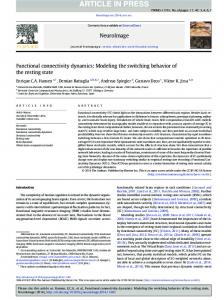
We used PPI to describe how functional connectivity between brain regions was altered as a result of psychological context (Friston et al., 1997). We hypothesized that the habenula showed greater PPI with the VTA and SN during SE compared to SS trials. With the contrast SE > SS, we identified a mask of the habenula comprising two symmetric spheres each of 6 mm in radius and centered at MNI coordinates [−1, −25, 1] and [1, −25, 1]. This mask was well within the area identified as habenula in Ullsperger and von Cramon, 2003 (Talairach and approximate MNI coordinates: [−5/6, −25, 8] and [−6/6, −25, 5]). On the basis of the GLM, we extracted the time series of the first eigenvariate of the BOLD signal of the habenula for each individual subject. The eigenvariate value, inside a region of interest (ROI), corresponds to the average BOLD signal weighted by the voxel significance, and it is more robust to outliers (Gitelman et al., 2003). This time series constituted the physiological variable. The time series were de-convolved to remove the effects of HRF, multiplied by the psychological variable (SE > SS, i.e., “1” for SE and “−1” for SS conditions), and re-convolved with the canonical HRF to obtain the interaction term or PPI variable (Gitelman et al., 2003). The three variables were entered as regressors in a whole-brain GLM. PPI analysis was performed for each individual subject, and the resulting positive contrast images (i.e., “1” for the PPI regressors) were used in random-effect group analysis (Penny et al., 2004). Group results were reported for p  SS, we also used SE > G and SS > G as psychological variables of PPI for comparison. To ascertain the specificity of brain regions of PPI with the habenula during error processing, we performed another PPI analysis with a “control” seed region, involving the error activated thalamic cluster (MNI coordinates [14, −12, 5] and [−14, −20, 10], 5,600 mm3), exclusively masked by a larger area encompassing the habenula (two spheres of 10 mm in radius and centered at [−1, −25, 1] and [1, −25, 1]). This mask was to ensure the exclusion of the habenula from the control seed region. For the regression slope analysis, multivariate GCA, and mediation analysis, we referred to the habenula and the regions identified with PPI as the ROIs or only the latter brain regions as ROIs. Multivariate Granger Causality Analysis

The analysis of PPI identified areal interaction but did not specify the direction of influence. In order to confirm our hypothesis that the habenula signals the VTA in error detection and not the other way around, we used a multivariate GCA (Stilla et al., 2007; Deshpande et al., 2009) to examine the direction of the influence between the ROIs of PPI and the habenula. Multivariate GCA was implemented as in our previous work (Duann et al., 2009; Ide and Li, 2011). We considered two models; the first one included the habenula and all four regions identified from PPI as ROIs, and the second model included the habenula and three PPI regions (all except the globus pallidus; see below). Multivariate GCA was performed for individual subjects. For each subject and each ROI, a summary time series was computed by averaging across voxels inside the ROI for each time point. These average time series were concatenated across four sessions, after de-trending and normalization (Ding et al., 2000). Afterward, the pre-processed

Frontiers in Human Neuroscience

time series were entered into multivariate autoregressive (MAR) modeling (Harrison et al., 2003). We used the Akaike Information Criterion (AIC), which imposes a complexity penalty on the number of parameters and avoids over-fitting of the data (Akaike, 1974). The application of MAR modeling required that each ROI time series was covariance stationary, which we examined with the Augmented Dickey Fuller (ADF) test (Hamilton, 1994). The ADF test verified that there was no unit root in the modeled time series. The residuals of MAR modeling were used to compute the Granger causality measures (F values) of each possible connection between ROIs. Since MAR modeling often involves highly interdependent residuals (Deshpande et al., 2009), we used permutation resampling (Hesterberg et al., 2005; Seth, 2010) to obtain an empirical null distribution of no causality, as suggested in Roebroeck et al. (2005), in order to estimate the Fcritical, and assess the statistical significance of Granger causality measures. With resampling, we produced surrogate data by randomly generating time series with the same mean, variance, autocorrelation function, and spectrum as the original data (Theiler et al., 1992), as implemented in previous EEG (Kaminski et al., 2001; Kus et al., 2004), and fMRI studies (Deshpande et al., 2009). We used binomial test to assess statistical significance in group analysis (Duann et  al., 2009; Uddin et  al., 2009); for each connection, we counted the number of subjects that had F > Fcritical (i.e., significant connection) and estimated its significance using a binomial distribution with parameters n = 59 trials and p = q = 0.5 (same probability to observe a connection or not). Multiple comparisons were corrected for false discovery rate (FDR; Genovese et al., 2002). We applied the same multivariate GCA procedures to resting state data of the 30 subjects, following our previous work (Duann et al., 2009), as an additional control for false positive connectivities. The absence of functional connectivity in the resting data would suggest that the task-related connectivity is not an artifact of HRF variability across the brain (see next section for more details). GCA: methodological considerations

Although some investigators argued the importance of causality based on temporal precedence and the utility of GCA in connectivity analyses (e.g., Roebroeck et al., 2009), others discussed the limitations of GCA (e.g., Friston, 2009). As detailed in a recent review of GCA in neuroimaging (Bressler and Seth, 2010), the utility of Granger causality measures depends on successfully estimating autoregressive (AR) models of stochastic processes. Successful applications of GCA to fMRI data (Roebroeck et al., 2005; Stilla et al., 2007; Bressler et al., 2008; Deshpande et al., 2009; Duann et al., 2009; Kayser et al., 2009; Ide and Li, 2011) appeared to have some elements in common. First, it is crucial that the modeled time series are wide-sense stationary (WSS; i.e., they have constant mean and variance). Otherwise, non-stationary time courses are known to produce spurious regression results (Granger and Newbold, 2001). Second, it is also important to have a number of observations (time points) adequate to estimate the AR model coefficients. In the current GCA modeling, by concatenating BOLD time series across four sessions for each individual (a total of 1,180 time points) after de-trending and normalization, we obtained time series (averaged inside each ROI) that were sufficiently long and covariance stationary, the latter verified by the ADF test. Third, we applied spatial

www.frontiersin.org

March 2011  |  Volume 5  |  Article 25  |  3

Ide and Li

Habenula and error processing

but not temporal filtering to the original BOLD signals because temporal (e.g., bandpass) filtering is known to introduce severe confounds in GCA of neuroimaging time series (Florin et al., 2010; Seth, 2010). These procedures were also successfully applied in our previous studies (Duann et al., 2009; Ide and Li, 2011). An additional consideration is the effects of HRF variability and down-sampling of BOLD signals on autoregressive modeling. A popular approach is to use the “difference of influence” (DOI) between two regions (Roebroeck et al., 2005; Stilla et al., 2007) to ameliorate these effects. However, this approach is no longer valid for multivariate GCA. In such cases, a useful practice is to analyze Granger causality during different experimental conditions (e.g., by studying both task and resting conditions; Duann et al., 2009; Kayser et al., 2009), since the effects of HRF variability and signal down-sampling are not expected to vary across conditions. A few studies in the literature presented less successful results from GCA. In a study of simultaneous electroencephalographic recordings and fMRI in rats, David et al. (2008) showed spurious connectivities derived from GCA due to HRF variability. However, one should note that the HRF variability was outside normal physiological range. Furthermore, in a recent investigation using simulated BOLD signals by convolving a standard HRF with local field potentials recorded from macaque cortex, Deshpande et al. (2010) showed that, even considering real and normal range of HRF variability (Handwerker et al., 2004) and a signal-to-noise ratio of 1 unit and a TR = 2 s, GCA reliably detected neuronal delays around 700 ms (Deshpande et al., 2010). Witt and Meyerand (2009) reported poor performance of GCA but it is not clear whether these experiments were biased because of simulated fMRI time series generated using Dynamic Causal Modeling (Friston, 2009) or whether these simulated time series were covariance stationary. Taken together, although GCA presents some technical challenges, we believe that, when it is carefully applied and done without over-interpretation of the results, GCA is a useful exploratory tool to delineate effective connectivity of the complex human brain. We performed mediation analyses to further characterize functional connectivity between the ROIs (MacKinnon et al., 2007), using the toolbox M3, developed by Tor Wager and Martin A. Lindquist1. Mediation analyses are widely used in social and economic research to examine whether a relationship between two variables is mediated by an intervening variable (Maccorquodale and Meehl, 1948; Baron and Kenny, 1986). It was successfully applied to fMRI of emotion regulation (Wager et al., 2008; Lebrecht and Badre, 2008) and more recently to analyses of functional connectivity (Hare et al., 2010). In a mediation analysis, the relation between the independent variable X and dependent variable Y, i.e., X → Y, is tested to see if it is significantly mediated by a variable M. The mediation test is performed by employing three regression equations (MacKinnon et al., 2007): Y = i2 + c′X + bM + e2 M = i3 + aX + e3 1

http://www.columbia.edu/cu/psychology/tor/

Frontiers in Human Neuroscience

Mediation analyses: methodological considerations

As with other methods based on structural equation models, one assumed that all relevant variables are included in the analysis; i.e., one could not rule out the existence of mediating factors not tested in the model (Lebrecht and Badre, 2008). In addition, mediation analysis is only valid upon correct specification of the causal orders (MacKinnon et al., 2007). We believe that these limitations were addressed to a significant extent in the current study: wholebrain PPI identified all relevant ROIs functionally connected to the habenula during errors; and multivariate GCA provided important information regarding causal orders. Finally, as pointed out by Wager et al. (2008), an additional limitation of using mediation analysis in fMRI is that models are made on the basis of naturally occurring variance over subjects, and thus conclusions are made with the assumption that inter-subject variability does not affect the coupling between dependent variables. This restriction also applies to the study. One could control the variability by simply removing the regression outliers (Chatterjee and Hadi, 1986) or, alternatively, develop multilevel mediation models that consider the mediation path coefficients as random effects (MacKinnon et al., 2007).

Results

Mediation analysis

Y = i1 + cX + e1

where a represents X → M, b represents M → Y (controlling for X), c′ represents X → Y (controlling for M), and c represents X → Y. In the literature, a, b, c, and c′ were referred as path coefficients or simply paths (MacKinnon et  al., 2007; Wager et  al., 2008), and we followed this notation. Variable M is said to be a mediator of connection X → Y, if (c − c′) is significantly different from 0, which is mathematically equivalent to the product of the paths a × b (MacKinnon et al., 2007). If the product a × b and the paths a and b are significant, one concludes that X → Y is mediated by M. In addition, if path c′ is not significant, it indicates that there is no direct connection from X to Y and that X → Y is completely mediated by M. Note that path b is the relation between Y and M, controlling for X, and it should not be confused with the correlation coefficient between Y and M.

Brain regions of PPI with the habenula

With general linear modeling we examined and confirmed errorrelated regional brain activations during the stop signal task (Li et al., 2008b). Compared to SS, SE trials evoked greater activations in the medial frontal cortex including the dorsal anterior cingulate cortex (dACC) and pre-supplementary motor area (preSMA), as well as the anterior inferior insulas, thalamus, habenula, and structures in the midbrain, at p  G) as well as posterior cingulate cortex and the precuneus (G > SS), p  SS (in cold color) in the stop signal task. T maps were thresholded at p