The common techniques to recover lost blocks are grouped under Automatic ... lost data. In Wada's work,. 1 error concealment approaches have assumed that ...
Error Resilient Video Coding With Improved 3-D SPIHT and Error Concealment Sungdae Choa and William A. Pearlmana a Center
for Image Processing Research Department of Electrical, Computer, and Systems Engineering Rensselaer Polytechnic Institute Troy, New York 12180-3590
ABSTRACT This paper first introduces an asymmetric tree structure for utilization with an error resilient form 3-D SPIHT, called ERC-SPIHT. Then, we present a fast error concealment scheme, borrowed from Rane et al.’s work with images, for embedded video bitstream using ERC-SPIHT. In addition to using simple averaging method in the root subband, we detect the presence or absence of edges in the lost block of every image. Then we use an interpolation scheme to recover the lost edge information. Keywords: video compression, 3-D wavelet transform, video transmission, embedded bitstream, asymmetric tree, error resilience, error concealment, SPIHT
1. INTRODUCTION The common techniques to recover lost blocks are grouped under Automatic Retransmission Query Protocols (ARQ). However, ARQ lowers data transmission rates and can further increase the network congestion which can aggravate the packet loss. For MPEG encoded video bitstreams, there were many attempts to conceal lost data. In Wada’s work,1 error concealment approaches have assumed that both encoding and decoding occur simultaneously, with the decoder communicating to the encoder the location of damaged picture blocks. Many of these techniques are not realistic for real-time applications since they require retransmission of ATM cells. Prioritization approaches to ATM cell loss concealment have been proposed.2,3 Techniques involving interleaving data have also been proposed,4,5 along with postprocessing techniques for error concealment.6–8 In all of these techniques, there has been no mention of how the loss of macroblocks is detected. Two error recovery approaches for MPEG encoded video over ATM networks are described by Salama.9 The first approach aims at reconstructing each lost pixel by spatial interpolation from the nearest undamaged pixels. The second approach recovers lost macroblocks by minimizing intersample variations within each block and across its boundaries. In wavelet-based encoded images for error concealment, Rogers and Cosman were able to group a variable number of blocks in one packets using packetizable zerotree wavelet (PZW) compression scheme.10 In the event of packet loss, 8 neighbors of the missing trees are present, because each packet is composed of trees come from widely dispersed locations using recursive tessellation technique.11 Then, the interpolation method is used to conceal the lost wavelet coefficients. Rane et al.12 also developed an algorithm claimed to be compatible with the wavelet-based JPEG 2000 image compression standard. Instead of using common retransmission query protocols, the researchers reconstruct the lost blocks in the wavelet-domain using the correlation between the lost block and its neighbors. The algorithm first uses a simple method to determine the presence or absence of edges in the lost block. This is followed by an interpolation scheme, designed to minimize the blockiness effect, while preserving the edges or texture into the interior of the block. In previous work,13 we used the average values of surrounding coefficients for the missing coefficients only in the spatio-temporal root subband. This method conceals lost coefficients in the background very successfully. However, the decoded sequence still suffers from loss of edge information, because this method does not conceal loss of high frequency information in higher level subbands, where the wavelet coefficients contain most of the edge information.
Contiguous Grouping
11 00 00 11 00 11 00 11 00 11 000 111 00 11 000 111 00 11 00 11 00 11 00 11 00 11 000 111 00 11 000 111 00 11 00 11 00 11 00 11 00 11 00 11 00 11 00 11 00 11 000 111 00 11 000 111 00 11 00 11 00 11 00 11 00 11 00 11 00 11 00 11 00 11 00 11 00 11 00 11 000 111 00 11 000 111 00 11 00 11 00 11 00 11 00 11 0011 11 0011 0011 11 00 000 111 00 11 000 111 00 11 00 11 00 11 00 000 111 00 11 000 111 00 11 00 11 000 111 00 11 000 111 0011 11 000011 0011 11 00 000 111 00 11 000 111 00 11 000 111 00 11 000 111 00 11 000 111 00 11 000 111 00 11 00 11 00 11 00 11 00 11 000 111 00 11 000 111 00 11 00 11 00 11 00 00 111 11 000 00 11 000 111 00 11 000 111 00 11 000 111 00 11 00 11 00 11 00 11 00 11 000 111 00 11 000 111 00 11 0011 11 0011 0011 11 00 00 11 00 11 00 11 00 11 000 111 00 11 000 111 00 11 00 11 00 11 00 11 00 111 11 000 111 00 11 000 111 00 11 00 11 00 11 00 11 00 11 000 00 11 000 111 00 11 00 11 00 11 00 11 00 111 11 000 00 11 000 111 00 11 00 11 00 11 00 11 00 111 11 000 00 11 000 111 00 0011 11 0011 0011 00 11 00 11 00011 111 00 000 111 00 11 00 11 00 11 00 11 00 11 000 111 00 11 000 111 00 11 00 00 00 00 11 000 111 00 000 111 0011 11 0011 11 0011 11 00 11 00 11 00011 111 00 11 000 111 00 11 00 11 00 11 00 11 00 11 000 111 00 11 000 111 00 11 00 11 00 11 00 11 000 111 00 11 000 111 00 11 00 11 00 11 00 11 00 11 00 11 000 111 00 11 000 111 00 11 00 11 00 11 00 11 000 111 00 11 000 111 00 11 00 11 00 11 00 11 00 11 000 111 00 11 000 111 00 11 00 11 00 11 00 11 00 11 000 111 00 11 000 111 00 11 00 11 00 11 00 11 00 11 000 111 00 11 000 111 00 11 11 00 00 11 00 11 00 11 00 11 00 11 00 11 00 11 00 11 00 11 00 11 00 11 00 11 00 11 00 11 00 11 00 11 00 11 00 11 00 11 00 11 00 11 00 11 00 11 00 11 00 11 00 11 00 11 00 11 00 11 00 11 00 11
111 000 00 11 000 111 00 11 000 111 00 11 000 111 00 11 000 111 00 11 000 111 00 11 000 111 00 11 000 111 00 11 000 111 00 11 000 111 00 11 000 111 00 11 000 111 00 11 000 111 00 11 000 111 00 11 000 111 00 11 000 111 00 11
Dispersive Grouping
111 000 000 00 000 000 111 000 111 000 111 00 11 000111 111 000 11 111 00111 11 00011 111 000 111 000 111 000 111 00 11 00 00 11 00 11 000 111 000 111 000 111 000 111 00 11 00 11 00 11 00 11 000 111 000 111 000 111 00 11 000 111 00 11 00 11 00 11 000 111 00 11 00 11 00 11 000 111 000 111 000 111 00 11 000 111 00 11 00 11 00 11 000 111 000111 111 000 11 00111 00011 000 111 00011 111 00011 111 00 00 00 11 00 000 111 000 111 000 111 00 11 000 111 000 111 000 111 000 111 00 11 000 111 000 00 000 000 111 000 111 000 111 00 11 000111 111 000 11 111 00111 11 00011 111 00 00 11 00 11 000 111 00 11 00 11 00 11 000 111 000 111 000 111 000 111 00 11 000 111 000 111 00 11 000 111 00 11 00 11 00 11 000 111 00 11 00 11 00 11 000 111 00 00 11 00 11 000 111 000111 111 000 11 00111 00011 00 11 00 11 00 11 000 111 00 00 11 00 000 111 00 11 000 111 111 000 00011 111 000 111 00011 111 00011 111 00 00 11 000 111 000 111 000 111 000 111 000 111 000 111 00 11 000 111 000 111 000 111 00 11 00 11 00 11 00 11 000 111 00 11 000 111 000 111 000 111 000 111 000 111 000 111 00 11 000 111 000 111 000 111 00 11 00 11 00 11 00 11 000 111 000 111 000 111 000 111 00 11 00 11 00 11 00 11 000 111 000 111 000 111 111 000 111 00 11 00 11 00 11 00 11 000 111 000 111 000 111 00 11 00 11 00 11 00 11 000 111 000 111 000 000 111 000 111 00 11 00 11 00 11 00 11 000 111 000 111 000 111 111 000 00 11 00 00 11 00 000 111 00 11 000 111 000 111 00011 111 000 111 00011 111 00011 111 00 00 11 000 111 000 111 000 111 000 111 000 111 000 111 00 11 000 111 000 111 000 111 00 11 00 11 00 11 00 11 000 111 00 11 000 111 000 111 000 111 000 111 000 111 000 111 00 11 000 111 000 111 000 111 00 11 00 11 00 11 00 11 000 111 000 111 000 111 111 000 111 00 11 00 11 00 11 00 11 000 111 000 111 000 111 000 00 11 00 11 00 11 00 11 000 111 111 000 11 000 111 000 111 000 00 111 00 11 000 111 000 111 000 11 111 00 000 111 000 111 000 111 00 11 000 111 000 111 000 11 111 00 000 111 000 111 000 11 111 00 000 111 000 111 000 111 00 11 000 111 000 111 000 11 111 00 000 111 000 111 000 11 111 00 000 111 000 111 000 111 00 11 000 111 000 111 000 11 111 00 000 111 000 111 000 11 111 00 000 111 000 111
111 000 000 111 111 000 00 11 000 111 000 111 111 000 00 11
11 00 00 11 00 11 00 11
11 00 000 111 00 11 000 111
Figure 1. Graphical illustration of the two grouping methods In this paper, we first introduce the ERC-SPIHT coding method and then its utilization with an asymmetric tree structure. This ERC-SPIHT with asymmetric tree structure gives a little higher compression ratio than that of the ERC-SPIHT with normal (symmetric) tree structure. Then, we apply the idea of Rane et al. to ERC-SPIHT. This method can detect presence or absence of edge information in the lost block of decoded image. In addition to that, we change the order of spatio-temporal wavelet transformation. Through this change, we can conceal the lost blocks in each frame separately. We also expand this idea to color ERC-SPIHT with asymmetric tree structure. The organization of this paper is as follows: Section 2 shows background of ERC-SPIHT. Section 3 describes Asymmetric Tree Structure of ERC-SPIHT. Section 4 explains the error concealment method. Section 5 provides simulation results, and Section 6 concludes this paper.
2. BACKGROUND OF ERC-SPIHT ERC-SPIHT13 uses a new method for partitioning the wavelet coefficients into s-t blocks. The 3-D SPIHT compression kernel is independently applied to each tree rooted in the wavelet coefficients in the lowest subband and branching to the spatially related coefficients in the higher frequency subbands. The algorithm produces sign, location and refinement information for the trees in each pass. Therefore, we need to keep intact the spatio-temporal related trees to maintain compression efficiency of the 3-D SPIHT algorithm. However, we do not have to keep together the contiguous wavelet coefficients in the lowest subband, since the kernel is independently applied to each tree rooted in a single lowest subband coefficients and branching into the higher frequency subbands at the same s-t orientation. In the ERC-SPIHT algorithm, therefore, we group the lowest subband coefficients at some fixed interval instead of grouping adjacent coefficients. This interval is determined by the number of s-t blocks S, the image dimensions, and number of decomposition levels. Then, we track the spatio-temporal related trees of the coefficients, and merge them together. Figure 1 illustrates the two methods of contiguous and dispersive grouping in the lowest subband. ERC-SPIHT generates some number S of different groups with this dispersive grouping, and then encodes each group independently using the 3-D SPIHT algorithm, so that S independent embedded 3-D SPIHT substreams are created. The S sub-bitstreams are then interleaved in appropriate fixed size units (e.g. bits, bytes, packets, etc.) prior to transmission so that the embedded nature of the composite bitstream is maintained. Therefore we can stop decoding at any compressed file-size or let run until nearly lossless reconstruction is obtained. The main advantage of the ERC-SPIHT dispersive grouping is the gaining of error resilience while maintaining coding efficiency. All of the sub-blocks contain similar information about each other, since each of the sub-blocks is composed of the coefficients not from a connected local region, but dispersed over the global region. Therefore, assignment of the same bitrates to each substream is nearly optimal in this method. Another nice feature of
H
LH LL Figure 2. Asymmetric Tree Structure the ERC-SPIHT is that the very early decoding failure affects the whole encoded region because the decoded coefficients would be spread out to the whole area along the sequence, and the defective coefficients can be concealed by the other surrounding coefficients which are decoded at a higher rate. Therefore, ERC-SPIHT does not suffer from small local areas which are decoded with lower bitrate.
3. ASYMMETRIC TREE STRUCTURE OF ERC-SPIHT 14,13
In previous works, we have used the 3-D SPIHT compression kernel with the tree structure introduced by Kim et al.15 This tree structure is just a simple extension of the symmetric 2-D SPIHT tree structure. Other researchers have proposed a more efficient tree structure.16,17 The main idea of the tree structure is to make the trees longer. The 3-D SPIHT algorithm is a tree-based coder, and tree-based coders tend to give better performance when the tree depth is long and the distribution is lopsided, since that increases the probability of a coefficient value being zero as we move from root to leaves. To make that kind of tree, we can simply decompose into more levels. We can not always do so, since there is a limitation according to the image size and GOF size. On the other hand, the asymmetric tree structure always gives a longer tree than that of the normal 3-D SPIHT. Figure 2 shows the asymmetric tree structure. In this figure, we assume that there are eight frames, and the frames are spatially and temporally transformed in two levels. As we can see, the new tree structure has 2 × 2 wavelet coefficients element in root subband (LL) rather than 2 × 2 × 2 wavelet coefficients element. Figure 3 graphically compares the tree structures among 2-D original tree structure after 2 level spatial decompositions, 3-D original tree structure after 2 level wavelet packet decompositions, and 3-D asymmetric tree structure after 2 level wavelet packet decompositions. As we can see, the asymmetric tree structure in each coefficient frames is exactly same as the 2-D SPIHT tree structure except that the top-left coefficient of each 2 × 2 group in LL and LH bands is part of a tree group. In 2-D SPIHT, the top left coefficient of each 2×2 group in the lowest subband is not part of any tree. On the other hand, the top-left coefficient of each 2 × 2 group in the lowest spatial subband in asymmetric tree structure
x *
y
t
t x
x
y
y
Ht
Ht
LHt LL t
LHt LL t
Figure 3. Comparison of tree structures (a)Top : 2-D original tree structure after 2 level spatial decomposition (b)Bottom-left : 3-D original tree structure after 2 level wavelet packet decomposition (c)Bottom-right : 3-D asymmetric tree structure after 2 level wavelet packet decomposition is linked with the 2 × 2 offspring group in the same spatial location of the following temporal subband, except the highest temporal subband. This means that the three coefficients of 2 × 2 group are linked with the 2 × 2 offspring group in the same coefficient frame, and one in another frame. As we can see in Figure 2, the top-left coefficient of each 2 × 2 group in the lowest spatial subband of temporal LL band has one 2 × 2 offspring group in temporal LH band, and the top-left coefficient of each 2 × 2 offspring group in the lowest spatial subband of temporal LH band has two 2 × 2 offspring group in temporal H band. This means that the top-left coefficients in LL and LH band are linked with the coefficients which represent the same spatial location in the following temporal subband. Therefore, the top-left coefficient of each 2 × 2 offspring group in the lowest spatial subband of temporal H band does not have any offspring, because there are no more temporal subbands. In this manner, the first stage of the tree is constructed. These are shown in Figure 2 by the arrows. To grow the tree further, each coefficient group is linked with each spatial subband, the same as with original 2-D SPIHT. Therefore, each 2 × 2 coefficient group in the lowest spatial subband of temporal LL band has three 2 × 2 offspring groups in temporal LL and one 2 × 2 offspring group in the LH band, and each 2 × 2 offspring group in the lowest spatial subband of temporal LH band has three 2 × 2 offspring groups in temporal LH and two in the H band. Each 2 × 2 offspring group in the lowest spatial subband of temporal H band has three 2 × 2 offspring groups in the same temporal H band, because it is the highest frequency subband.
Encoder Temporal Decomposition
Spatial Decomposition
3-D SPIHT Encoder
Noisy Channel
Temporal Transform
Spatial Transform
Conceal Root Subband
Decoder Figure 4. Block diagram of of 3-D SPIHT encoding/decoding structure with normal order of wavelet transformation and error concealment
4. ERROR CONCEALMENT METHOD In previous work,13 we concealed the missing blocks only in the spatio-temporal root subband using the average value of coefficients surrounding the lost coefficients before the inverse wavelet transformation. Figure 4 shows the block diagram of this step. The concealment is done just before the inverse spatio-temporal wavelet transformation. In sixteen frames with three levels of spatio-temporal decomposition, the root subband comprises the first two wavelet coefficient frames. As we saw in previous work,13 root subband averaging successfully recovered most of the background image. However, we could not recover the detail information of the image when the missing block contains an edge. Now we change the order of spatial and temporal transformation as in Figure 5, so that spatial transformation precedes temporal transformation in the encoder and follows it in the decoder. Any early decoding failure or missing substream affects the related spatio-temporal tree block in the wavelet domain, and the block affects a full GOF (Group Of Frames). The similar idea was used in the coding of Region of Interest (ROI) associated with the STTP-SPIHT algorithm by Cho and Pearlman.18 As we can see, the corresponding coefficients of all the spatio-temporal orientation trees in any substream are located in the same spatial location in each frame of coefficients. Therefore, inverse temporal transformation will not affect other cleanly recovered coefficients, because the transformation uses a 1-D filter only in the temporal direction. In the decoder, therefore, we apply the concealment step right after the inverse temporal transformations. The next step is the inverse spatial transformation, and this transformation is applied to each individual frame of coefficients. In this way, we can conceal the error effects in the root subband in each frame rather than conceal only those in the spatio-temporal root subband as in previous work.13 As we know, 3-D SPIHT uses the 2 × 2 × 2 coefficient group as a basic element. In previous work,13 we kept the 2 × 2 × 2 coefficient group together in both spatial and temporal directions. Therefore, if any substream is missing, there are twelve coefficients surrounding each 2 × 2 coefficient group in each coefficient frame. In this paper, however, we interleave the coefficients with fixed interval I0 in the lowest spatial subband of each coefficient frame to get the 2×2 coefficient group. Figure 6 shows the comparison of missing coefficients’ positions and its surrounding coefficients in the case of 16 × 16 lowest spatial subband when the number of substream S is sixteen. Therefore, there are 256 coefficients, and each substream is composed of 16 coefficients in this
Encoder Spatial Decomposition
Temporal Decomposition
3-D SPIHT Encoder
Noisy Channel
Spatial Transform
Conceal Root + High on Each Frame
Temporal Transform
Decoder Figure 5. Block diagram of 3-D SPIHT encoding/ decoding structure with different order of wavelet transformation and error concealment subband. As a result, if one of substream is missing, then sixteen coefficients in this subband are affected. In this figure, the black pixels represent the missing coefficients. Figure 6 (a) illustrates the missing coefficients and its surrounding coefficients in the case of 2 × 2 contiguous grouping that was used in previous work.13 As we can see, there are twelve surrounding coefficients in each 2 × 2 group. For the 2 × 2 interleaved grouping, there are 32 spatially surrounding coefficients in the lowest spatial subband of each coefficient frame for every 2 × 2 coefficient group. Figure 6 (b) illustrates this idea. These steps give about 1 dB better performance than that of previous work13 when one of the subbitstreams is completely missing. However, there are still some blocks which are not successfully recovered by this lowest spatial subband concealment in each coefficient frame. Most unrecovered blocks are parts of edges, and the edge information is in the high frequency subbands. Therefore, it is inevitable to conceal in the high frequency subbands to recover detailed information of the image. As in Rane et al.,12 we utilize concealment in the high frequency subband in addition to the root subband concealment. The magnitude of a wavelet coefficient in a specific location tells both the amount of change and the spatial location at which the change occurs. Each level of the wavelet transform domain has three different subbands except at the lowest level, and each subband has different characteristics, such as vertical (V), horizontal (H), or diagonal (D) detail. Figure 7 (a) shows this idea for a three level decomposed image. As we explained in previous sections, we use 2×2 interleaved coefficient group as shows in Figure 6. Therefore, any missing block affects one coefficient with a fixed interval, I0 , in V0, H0, and D0 level, 2 × 2 coefficient group with a fixed interval, I1 = 2×I0 , in V1, H1, and D1 level, and 4 × 4 coefficient group with a fixed interval, I2 = 4×I0 , in V2, H2, and D2 level. In this figure (b), the interval I0 = 4 for S = 16 substreams. To recover the lost edge information, we test the missing block to see whether the block contains part of an edge or not. In Figure 7 (b), we show an example of a test of vertical edges in V1 level. A missing substream affects the 2 × 2 coefficient group with a fixed interval I1 in V1 level. In that case, we just need the right above and right below coefficients of the missing blocks, and test whether the values are greater than certain threshold value. If any of four tests meets the condition, then we decide the missing block is in part of vertical edge, and apply linear least squares interpolation. Analogously, the coefficients left and right of the missing block
I0
Figure 6. Comparison of position of tree head and its surrounding coefficients in root subband of size 16 × 16. (a) Left : 2 × 2 contiguous grouping, (b) Right : 2 × 2 interleaved grouping are needed to recover horizontal detail, and diagonal neighboring coefficients are needed to recover the diagonal detail. ˆ = mA1 +nA2 , here A1 For each high frequency subband, the matrix estimate of lost coefficients is given by X and A2 are the adjacent coefficient, and m and n are scalar parameters. In the vertical edge case as in Figure 7, A1 and A2 can be T (Top) and B (Bottom) respectively. Then, we need to find m and n where the error at the top and bottom borders is minimized. For V 0 level, once we decide the lost block is in part of vertical edge, the m and n are simply means, that is the average value of right above and right below coefficients. For V 1 level, we can just set � ˆ= X Then, we solve for
xˆ12 xˆ22
x ˆ 11 x ˆ21 �
x ˆ11 x ˆ12
�
� ,T =
�
� =m
t11 t21 t11 t12
t12 t22
�
�
� ,B =
� +n
b11 b12
b11 b21
b12 b22
�
�
� � � � �2 � t21 xˆ11 � �ˆ ˆ and T . − T where X = that minimizes �t = �X t b� t b= xˆ12 t22 We also find xˆ21 and xˆ22 to minimize the squared error at the bottom border, i.e we solve � � � � � � x ˆ 21 t21 b21 =m +n x ˆ22 t22 b22 � � � � �2 � b11 x ˆ21 � �ˆ ˆ and B − B where X = to minimize �t = �X b t� b t= x ˆ22 b12 For the lost blocks in horizontal and diagonal edges, we can use the same equation above, and we just need to replace the T and B vectors with L (Left) and R (Right), or D1 (Upper Diagonal) and D2 (Lower Diagonal) vectors for the horizontal and diagonal edges, respectively. For level 2, we can still expand the equation above to estimate the lost coefficient in that level. However, in this thesis, we conceal errors only in level 1 and 2 in addition to those in the root subband. This additional high frequency subband concealment almost always gives successful reproduction of video over noisy channels even when some of substreams are totally missing.
DC
1 0
H0
10 01
0011
V0
V1
D0
01
1 0 0 1 H1
0000 1111 0000 1111 V2
D1
Missing Block
11 00 00 11 00 11 H2
Missing Block
Missing Block
Missing Block
000 111 000 111 D2
Figure 7. Graphical illustration of error concealment in the case of missing block is in part of vertical edge. (a) Left : Characteristics of vertical (V0, V1, V2), horizontal (H0, H1, H2) or diagonal (D0, D1, D2) detail in each subband, (b) Example : Test of vertical edge
5. RESULTS In this section, we provide the result of comparison between the 3-D SPIHT with symmetric tree structure and ERC-SPIHT with asymmetric tree structure in noiseless channel for both gray scale and color video sequences. In addition to that, we provide the PSNR results of different number of decomposition between the spatial and temporal dimensions. We also show the performance of the root plus high band error concealment of 3-D SPIHT with the asymmetric tree structure. Then, we provide the simulation results in noisy channel and compare the ERC-SPIHT with asymmetric tree with other error resilient methods that were introduced in previous paper.13 In our test of error resilience, we use the same channel conditions as in this previous work.18,13 For the ERCSPIHT with asymmetric structure, we use the above described concealment method for the missing substream and the substreams that have early decoding failure. For the edge test, we determine the threshold value after testing with a number of trials. This threshold value is used to see whether the missing block contains part of edge or not. For the ERC-SPIHT in this paper, we use 2 × 2 coefficient groups as a basic element, and we interleave the coefficients in the spatial domain to form the element as shown in Figure 6 (b). Table 1 shows the comparison of PSNRs (dB) in a noiseless channel among the MPEG-2, 3-D SPIHT with symmetric tree structure (3-D SPIHT [1]), 3-D SPIHT with asymmetric tree structure (3-D SPIHT [2]), ERC-SPIHT with symmetric tree structure (ERC-SPIHT [1]), asymmetric tree structure (ERC-SPIHT [2]), and asymmetric tree structure with different number of decomposition (ERC-SPIHT [3]), at total transmission rate of 2.53 Mbps. For the case of different number of decomposition, we kept the same number of temporal decomposition (three level), and used one more level (four) of spatial decomposition. As we can see, the PSNRs of ERC-SPIHT with asymmetric tree structure are about 0.1 - 0.3 dB higher than those of the ERC-SPIHT with symmetric tree structure, and the PSNRs of ERC-SPIHT with asymmetric tree structure and different number of decomposition are about 0.2-0.4 dB higher than those of the ERC-SPIHT with symmetric tree structure, and comparable to those of the original 3-D SPIHT. ERC-SPIHT with the same number of decompositions and the same tree structure as 3-D SPIHT will have slightly lower performance due to the extra overhead needed for sub-bitstream headers. When we compare with MPEG-2, the average PSNRs of ERC-SPIHT (S=16) with asymmetric tree structure are about 0.7 - 1.5 dB higher than those of the MPEG-2. Table 2 shows the comparison of PSNRs (dB) for 352×240×80 “Football” and “Table Tennis” color sequences (YUV 4:2:2) using 3-D SPIHT with a symmetric tree structure, ERC-SPIHT (S = 4, 16) with asymmetric tree structure, and MPEG-2 at total transmission rate of 2.53 Mbps in noiseless channel condition. The average
MPEG-2 3-D SPIHT [1] 3-D SPIHT [2] ERC-SPIHT [1] (S=16) ERC-SPIHT [2] (S=16) ERC-SPIHT [3] (S=16)
Football 33.27 34.20 34.33 33.64 33.96 34.01
Susie 42.90 44.66 44.72 44.13 44.31 44.36
Table 1. Comparison of PSNRs (dB) for 352 × 240 × 48 “Football” and “Susie” sequence (gray) using MPEG-2, 3-D SPIHT with symmetric tree structure (3-D SPIHT [1]), 3-D SPIHT with asymmetric tree structure (3D SPIHT [2]), ERC-SPIHT with symmetric tree structure (ERC-SPIHT [1]), with asymmetric tree structure (ERC-SPIHT [2]), and with asymmetric tree structure and different number of decompositions (ERC-SPIHT [3]), at total transmission rate of 2.53 Mbps in noiseless channel PSNR for luminance Y of ERC-SPIHT (S = 4) with asymmetric tree structure is only about 0.1-0.2 dB lower than that of the normal 3-D SPIHT, and the average PSNR for Y of ERC-SPIHT (S = 16) is about 0.3-0.4 dB lower. Chroma planes U and V components of ERC-SPIHT (S = 4) are just about 0.1 dB lower than that of the normal 3-D SPIHT in the case of Football sequence and slightly higher than that of the normal 3-D SPIHT in the case of Table Tennis sequence. For S = 16, U and V of ERC-SPIHT (S = 16) are just about 0.2 dB lower than that of the 3-D SPIHT with symmetric tree structure. When we compare with MPEG-2, the average PSNRs for Y of ERC-SPIHT (S=16) with asymmetric tree structure are about 0.5 - 1.5 dB higher than those of the MPEG-2 in the case of Football sequence, and about 0.3 dB higher than those of the MPEG-2 in the case of Table Tennis sequence. The U and V planes of ERC-SPIHT (S = 16) are about 0.2 - 0.7 dB higher than those of the MPEG-2 in the case of Football sequence, and about 0.2 - 0.8 dB lower than those of the MPEG-2 in the case of Table Tennis sequence.
1Mbps
2.53 Mbps
3-D SPIHT ERC-SPIHT (S = 4) ERC-SPIHT (S = 16) MPEG-2 3-D SPIHT ERC-SPIHT (S = 4) ERC-SPIHT (S = 16) MPEG-2
Y 29.63 29.39 29.15 28.50 34.90 34.69 34.49 32.92
Football U 38.43 38.32 38.22 38.06 40.86 40.76 40.65 39.96
V 36.36 36.19 36.05 35.79 39.64 39.56 39.42 38.67
Table Tennis Y U V 31.69 40.32 42.23 31.61 40.24 42.17 31.37 39.98 41.95 31.00 41.54 42.83 36.45 44.36 45.52 36.34 44.37 45.54 36.12 44.13 45.35 35.97 44.76 45.50
Table 2. Comparison of PSNRs (dB) for 352 × 240 × 80 color “Football” and “Table Tennis” sequence (YUV 4:2:2) using 3-D SPIHT with symmetric tree structure, ERC-SPIHT (S = 4, 16) with asymmetric tree structure, and MPEG-2 at total transmission rate of 2.53 Mbps in noiseless channel To show the performance of error concealment, we assumed the decoding error occurred in the beginning of the substream number 7 (seventh packet) for the 352 × 240 “Football” sequence as we showed in previous work.13 Figures 8 shows the sample sequence to compare the results after the error concealment. In all figures, left column shows the results from the ERC-SPIHT without error concealment, middle column the results with root subband error concealment, and right column the results with root and high subband error concealment. As we can see, in the case of no concealment, there are many black spots in the images. When we use only root subband concealment for the missing coefficients, we can recover the missing areas very well, but there are still some spots where recovery is not successful, and these spots are marked by rectangle. In Figure 8 (b), the player’s right shoulder, in (e), the player’s head and another players left shoulder, and in (h), the player’s same left shoulder and another player’s line on his uniform are not recovered successfully. In (c), (f), and (i) of the
figure, we can see the edges are nearly perfectly recovered by root and high subband concealment. To demonstrate the general performance of error resilient video transmission over noisy channels, we did simulations using ERC-SPIHT encoded bitstreams with the asymmetric tree structure. Table 3 shows the comparison of average PSNRs (dB) of 352 × 240 × 48 monochrome “Football” and “Susie” sequence over fifty (50) independent runs among 3-D SPIHT/RCPC, ERC-SPIHT/RCPC (S = 16) with asymmetric tree structure and error concealment, and MPEG-2/RCPC at total transmission rate of 2.53 Mbps with bit error rates (BER) of 0.01 and 0.001. As we can see, the ERC-SPIHT with asymmetric tree structure and error concealment gives very high PSNRs, and comparable result as the 3-D SPIHT with RCPC and ARQ method, which assumes that there exists an ideal return channel. Football 0.01 0.001 3-D SPIHT/RCPC 24.50 28.20 ERC-SPIHT (S = 16)/RCPC 30.23 31.81 3-D SPIHT/RCPC+ARQ 32.10 32.80 MPEG-2/RCPC ∗ 26.35 28.09 ∗ omits frames of failed decoding
Susie 0.01 0.001 34.46 37.64 40.31 41.76 41.71 43.23 36.66 38.87
Table 3. Comparison of average PSNRs (dB) of 352 × 240 × 48 gray “Football” and “Susie” sequence over 50 independent trials among 3-D SPIHT/RCPC, ERC-SPIHT/RCPC (S = 16) with asymmetric tree structure and error concealment, and MPEG-2/RCPC at total transmission rate of 2.53 Mbps with bit error rates (BER) of 0.01 and 0.001 Table 4 shows the comparison of average PSNRs (dB) of 352 × 240 × 48 color “Football” and “Table Tennis” sequence (YUV 4:2:2) over fifty (50) independent runs among 3-D SPIHT/RCPC, ERC-SPIHT/RCPC (S = 16) with asymmetric tree structure and error concealment, and MPEG-2/RCPC at total transmission rate of 1 Mbps and 2.53 Mbps with bit error rates (BER) of 0.01 and 0.001. We can find that the average PSNRs for Y of ERC-SPIHT (S = 16) are 1 to 2 dB higher in “Football” sequence and 0.5 to 2 dB higher in “Table Tennis” sequence, and U and V of ERC-SPIHT (S = 16) are 0.5 to 2 dB higher than that of MPEG-2 in noisy channel conditions. The MPEG-2 results are averages over the frames that were successfully decoded. There were no occurrences of frames that could not be decoded in the other simulations.
6. CONCLUSION In this paper, we showed that the ERC-SPIHT could achieve higher compression performance with asymmetric tree structure in noiseless channel condition. In addition to that, we demonstrated that we could get even higher PSNRs when we use a different number of decompositions between the spatial and temporal dimensions. Then we extend the gray scale ERC-SPIHT with asymmetric tree structure to color ERC-SPIHT with asymmetric tree structure. We also have implemented an error concealment method of embedded video which is encoded by ERC-SPIHT with asymmetric tree structure. It conceals most lost edge information as well as background. The concealment is obtained at a very low computational complexity. Therefore, it can be implemented in real time applications.
REFERENCES 1. M. Wada, “Selective recovery of video packet loss using error concealment,” IEEE Journal on Selected Areas in Communications (JSAC) 7, pp. 207–214, June 1989. 2. P. Pancha and M. E. Zarki, “Mpeg coding for variable bit rate video transmission,” IEEE Communications Magazine 32, pp. 54–56, May 1994. 3. M. Ghanbari and V. Sferidis, “Cell-loss concealment if atm networks,” IEEE Transactions on Circuits and Systems for Video Technology 3, pp. 238–247, June 1993. 4. Q. Zhu, Y. Wang, and L. Shaw, “Coding and cell loss recovery in dct based packet video,” IEEE Transactions on Circuits and Systems for Video Technology 3, pp. 248–258, June 1993.
BER
1Mbps
2.53 Mbps
3-D SPIHT/RCPC ERC-SPIHT/RCPC MPEG-2/RCPC ∗ 3-D SPIHT/RCPC ERC-SPIHT/RCPC MPEG-2/RCPC ∗ BER
3-D SPIHT/RCPC 1Mbps ERC-SPIHT/RCPC MPEG-2/RCPC ∗ 3-D SPIHT/RCPC 2.53 Mbps ERC-SPIHT/RCPC MPEG-2/RCPC ∗ ∗ omits frames of failed decoding
Football 0.01 Y U 26.02 36.69 26.69 37.24 26.13 36.68 26.44 36.88 30.47 39.06 28.58 37.14 Table Tennis 0.01 Y U 27.99 36.87 28.93 37.79 28.56 38.95 28.51 37.16 32.47 40.95 31.64 40.52
V 33.50 34.29 33.81 33.76 36.96 35.38
Y 26.67 27.93 26.92 27.60 32.04 29.70
0.001 U 37.05 37.78 36.85 37.49 39.79 37.77
V 34.04 35 22 34.30 34.64 38.00 36.21
V 39.19 40.15 40.72 39.43 42.80 42.28
Y 28.84 30.20 29.14 29.77 33.80 31.87
0.001 U 37.55 38.92 38.89 38.35 42.19 39.57
V 39.84 41.03 40.89 40.47 43.81 41.81
Table 4. Comparison of average PSNRs (dB) of 352 × 240 × 80 color “Football” and “Table Tennis” sequence (YUV 4:2:2) over 50 independent trials among 3-D SPIHT/RCPC, ERC-SPIHT/RCPC (S = 16) with asymmetric tree structure and error concealment, and MPEG-2/RCPC at total transmission rate of 1 Mbps and 2.53 Mbps with bit error rates (BER) of 0.01 and 0.001 5. A. S. Tom, C. L. Yeh, and F. Chu, “Packet video for cell loss protection using deinterleaving and scrambling,” IEEE International Conference on Acoustics, Speech, and Signal Processing , pp. 2857–2860, May 1991. 6. Y. Wang, Q. Zhu, and L. Shaw, “Maximally smooth image recovery in transform coding,” IEEE Transactions on Communications 41, pp. 1544–1551, October 1993. 7. H. Sun and J. Zdepski, “Adaptive error concealment algorithm for mpeg compressed video,” Proceedings of SPIE on Visual Communications and Image Processing (VCIP) , pp. 818–824, November 1992. 8. H. Sun and W. Kwok, “Concealment of damaged block transform coded images using projections onto conves sets,” IEEE Transactions on Image Processing 4, pp. 470–477, April 1995. 9. P. Salama, “Error concealment techniques for encoded video streams,” Proceedings of IEEE ICIP 1, pp. 9– 12, October 1995. 10. J. K. Rogers and P. C. Cosman, “Wavelet zerotree image compression with packetization,,” IEEE Signal Processing Letters, 5, pp. 105–107, May 1998. 11. R. Ulichney, “Digital halftoning,” MIT Press, Cambridge, Mass. , 1987. 12. S. Rane, G. Sapiro, and M. Bertalmio, “Wavelet domain reconstruction of lost blocks in wireless image transmission and packet-switched networks,” submitted to IEEE Transactions on Image Processing , 2002. 13. S. Cho and W. A.Pearlman, “Error resilience and recovery in streaming of embedded video,” Journal of Signal Processing 82, pp. 1545–1558, November 2002. 14. S. Cho and W. A.Pearlman, “A full-featured, error resilient, scalable wavelet video codec based on the set partitioning in hierarchical trees (spiht) algorithm,” IEEE Trans. on Circuits and Systems for Video Technology 12, pp. 157–171, March 2002. 15. B.-J. Kim, Z. Xiong, and W. A. Pearlman, “Low bit-rate scalable video coding with 3d set partitioning in hierarchical trees (3d spiht),” IEEE Trans. Circuits and Systems for Video Technology 10, pp. 1374–1387, December 2000. 16. P. L. Dragotti, G. Poggi, and A. R. P. Ragozini, “Compression of multispectral images by three-dimensional spiht algorithm,” IEEE Transactions on Geoscience and Remote Sensing 38, pp. 416–428, January 2000.
(a)
(b)
(c)
(d)
(e)
(f)
(g)
(h)
(i)
Figure 8. 352 × 240 “Football” sequence coded to 1.0 bit/pixel, with ERC-SPIHT (S = 16). (a) frame 0 : without concealment after the seventh substream is missing, PSNR = 17.69 dB, (b) with root subband concealment, PSNR = 30.91 dB, (c) with root + high subband concealment, PSNR = 30.93 dB, (d) frame 4 : without concealment after the seventh substream is missing, PSNR = 17.63 dB, (e) with root subband concealment, 31.07 dB, (f) with root + high subband concealment, 31.17 dB, (g) frame 7 : without concealment after the seventh substream is missing, PSNR = 17.60 dB, (h) with root subband concealment, 29.63 dB, (i) with root + high subband concealment, 29.64 dB 17. C. He, J. Dong, and Y. F. Zheng, “Optimal 3-d coefficient tree structure for the 3-d wavelet video coding,” Technical Report, HZ-2001, Wavelet Research Laboratory, Department of Electrical Engineering, Ohio State University , August 2002. 18. S. Cho and W. A.Pearlman, “Region-based spiht coding and multiresolution decoding of image sequences,” Proceedings of Picture Coding Symposium, PCS-2001 , pp. 283–286, April 2001.