Estimating Accuracy for Text Classification Tasks on Large Unlabeled Data Snigdha Chaturvedi
Tanveer A. Faruquie
L. Venkata Subramaniam
IBM Research India New Delhi, India
IBM Research India New Delhi, India
IBM Research India New Delhi, India
[email protected]
[email protected] Mukesh K. Mohania
[email protected]
IBM India Software Lab New Delhi, India
[email protected] ABSTRACT
1.
Rule based systems for processing text data encode the knowledge of a human expert into a rule base to take decisions based on interactions of the input data and the rule base. Similarly, supervised learning based systems can learn patterns present in a given dataset to make decisions on similar and other related data. Performances of both these classes of models are largely dependent on the training examples seen by them, based on which the learning was performed. Even though trained models might fit well on training data, the accuracies they yield on a new test data may be considerably different. Computing the accuracy of the learnt models on new unlabeled datasets is a challenging problem requiring costly labeling, and which is still likely to only cover a subset of the new data because of the large sizes of datasets involved. In this paper, we present a method to estimate the accuracy of a given model on a new dataset without manually labeling the data. We verify our method on large datasets for two shallow text processing tasks: document classification and postal address segmentation, and using both supervised machine learning methods and human generated rule based models.
Today, the quantity of available information is increasing exponentially. Enormous amounts of data is present within enterprises; and various standard techniques are increasingly being utilized to process this data automatically, such as for verification, data-cleansing, data-correction, forecasting and categorization. For example, let us consider the case of medium to large enterprises, which have millions of customer address records. For the sake of customer segmentation, it is often necessary to determine entities within these addresses such as street names, city names, state names and postal codes. The number of such records can be several millions for medium to large sized companies. In practice, rule based models, which encode human expert knowledge, are often employed for this purpose.[8] These rules based models can also be thought of as supervised systems where the expert generalizes rules to unseen situations. Whenever new data is presented to this trained model, one needs to customize the model according to properties of the new data by including new rules or modifying existing ones. This customization is an expensive task and hence, an estimation of the customization effort needed is essential in making policy decisions. A preliminary step in estimating customization effort requires knowledge of the accuracy of the existing uncustomized model on the new dataset. Even in case of machine learning models, one needs to know the accuracy of the model on a new dataset. The accuracy of a model may vary considerably from one dataset to another if the new dataset is drawn from a different underlying distribution. For example, a model built to recognize and classify address segment entities in postal addresses using examples from one geography may not perform satisfactorily for addresses from another geography. The present methods of accuracy computation involve manually labeling a subset of the new dataset and then calculating the accuracy of the model. However, manually labeling a dataset is usually a costly and time-consuming operation. Most often, only a very small fraction of the total data can be labeled. So, any trained model can only be tested on a few hundred manually labeled records out of hundreds of thousands and the trained model’s accuracy on this small subset has to be generalized to the complete dataset. Sometimes these samples are not sufficiently representative of the complete dataset, and this can later lead to incorrect deductions. While traditional techniques like cross validation
Categories and Subject Descriptors I.2.6 [Artificial Intelligence]: Learning—Knowledge acquisition
General Terms Management
Keywords Meta-learning, Accuracy Prediction, Regression, Text Classification, Address Segmentation
Permission to make digital or hard copies of all or part of this work for personal or classroom use is granted without fee provided that copies are not made or distributed for profit or commercial advantage and that copies bear this notice and the full citation on the first page. To copy otherwise, to republish, to post on servers or to redistribute to lists, requires prior specific permission and/or a fee. CIKM’10, October 26–30, 2010, Toronto, Ontario, Canada. Copyright 2010 ACM 978-1-4503-0099-5/10/10 ...$10.00.
INTRODUCTION
and holding out data can be used for fine tuning a model so as to better fit it on the data used for training, they represent the model’s performance on the available training data and their results cannot be generalized to predict model’s accuracy on any new test dataset coming from a different underlying distribution. It is then desirable to have a way of estimating the accuracy of a model on a new dataset without having to perform the actual labeling. In this paper we present a meta-learning approach to perform this task efficiently. Our method for estimating accuracy comprises of building a regression based predictor of accuracies. We train the accuracy prediction model on datasets with known accuracies, using an appropriate selection of meta-features characterizing the dataset. For example, to determine the house number token within a postal address, orthographic features such as the length of the token, capitalization patterns and relative positions can be used in making the identification. In this example, to estimate the accuracy of the segmentation model, which is the task of the accuracy prediction, we need to determine how effectively the segmentation model is able to find the house number tokens. We show that there are meta-features that can be used by the accuracy prediction model to estimate the segmentation model’s accuracy. In our experiments, we show that the approach of building an accuracy prediction model using meta-features is applicable to different decision models ranging from rule based systems to supervised machine learning algorithms. We validate our method on two important text processing tasks, i.e. postal address segmentation task and a supervised learning based text classification task. Also significantly, one would like to consider only a small subset of the data instead of processing the complete dataset consisting of millions of records. We present a sampling technique to efficiently choose representative samples from the huge test data and present method to estimate the accuracy on the complete data using these representative samples so as to avoid huge computational overheads. We empirically show that samples drawn using our method are more representative of the dataset than samples drawn using another popular technique, Simple Random Sampling. The rest of the paper is organized as follows. The next Section describes related work done in this domain and describes how the current study differs from the existing work. Section 3 describes our approach in detail. In Section 4 we discuss our experiments and results for two different types of text processing tasks, and using rule based models and machine learning algorithms. Section 5 concludes the study with a brief discussion of the work.
2.
RELATED WORK
It is well known that any machine learning algorithm cannot cater to needs of all types of problems. Most often, the machine learning practitioner chooses the algorithm to use by observing characteristics of the dataset at hand and then deciding the suitability of the available algorithms. Recently, attempts have been made to design models which can automatically perform such tasks via ‘meta-learning’. Meta-learning involves characterizing a dataset by a set of ‘meta-features’ and then designing models that make prediction about new datasets. The problem of dataset characterization has been addressed in some previous works. The major dataset characterization techniques include a set of
mean based statistical and information-theoretic measures of the attributes developed as a sequel to the work done in the STATLOG project [13], and a finer implementation of these measures in the form of histograms instead of means [10]. Another method which performs well is the landmarking approach [14] where a few selected well known algorithms are treated as landmarkers and the corresponding accuracies on the dataset under consideration are treated as measures to characterize the dataset. In this case, the landmarkers virtually measure some specific property of the dataset and a good performance of the landmarker is reflective of the property. These measures have been explored by several researchers in exploiting meta-learning in ways like ranking various available machine learning models in order of their suitability for the task; finding the best algorithm for the dataset from a pool of algorithms via a relative ordering of the algorithms [14] and predicting whether a particular algorithm is suitable for the dataset [13]. All these methods explore meta-learning as a classification task. In this paper we follow the approach of Bensusan and Kalousis [2] who investigate the use of meta-learning to directly estimate the predictive accuracy of a classifier. They develop regression models for predicting the accuracies of a set of 8 classifiers using three different data characterization techniques mentioned above. They empirically show that landmarking is the best performing method of dataset characterization, followed by the statistical and information theoretic measures and finally histogram based measures. Our work differs from theirs in the nature of targeted datasets. In their experiments, the datasets used are labeled and span varying domains. Hence they use very coarse metafeatures which measure the nature of attributes and labels eg. fraction of attributes that are nominal in nature, size of datasets, sparseness, number of labels, types of labels, performance of various landmarkers on the datasets etc. In our case, the datasets are largely from the same domain. Thus, the datasets and the attributes describing them are largely similar to each other. Also, the datasets are unlabeled and textual in nature. Due to lack of labels and largely overlapping feature-spaces, most meta-features used by Bensusan and Kalousis are not applicable for unlabeled textual data. For instance, in our case, landmarking, which is the dataset characterizing technique recommended by Bensuasan and Kalousis, is not applicable because the lack of labels prevents us from determining the accuracies of the landmarkers (few selected algorithms) on our dataset. Owing to the same reason, meta-features like number of labels and types of labels cannot be used in our case. Moreover, since the datasets in our case are described by the same set of attributes, meta-features like fraction of nominal attributes are rendered useless. Instead, we rely on finer metafeatures, for example measuring moments of distributions of attributes instead of just nature of attributes. We also find that the selected meta-features show significant correlations with accuracy, thus, justifying our approach. Furthermore, we apply this approach in a domain where the potential of meta-learning is yet unexplored as of now; possibly because of the inherent challenges that accompany text processing tasks, even though potential applications in this field are significant. We validate our method to estimate the accuracy of different types of decision models ranging from supervised machine learning models (like SVMs) to
human generated rule based models. We also show how such an approach can be used for relatively simpler tasks such as document classification as well as more complex tasks such as postal address segmentation where the method can becomes complicated when attempting to include context into the approach. Cieslak and Chawla [4] describe a series of measures to determine whether there is a significant difference in the two distributions which might lead to a difference in classifier performance and also identify the features responsible for this difference. However, they do not use this knowledge of difference in distribution to propose a modification in the estimate of classifier performances on different testsets. Other seemingly related popular machine learning techniques include Semi-supervised Learning [3], Transfer Learning [7] and Active Learning [6]. Semi-supervised learning aims at alleviating the problem of limited availability of labeled training data by utilizing the information present in unlabeled data. Transfer learning exploits the knowledge gained in solving a particular problem in solving problems belonging to other related domains. Similarly, in cases where labeled data is limited and labeling is costly, Active Learning tries to build learner in a more efficient manner by actively choosing the more informative data points to be labeled. All these techniques are designed to improve a classifier’s performance in scenarios where there is a lack of labeled data. Even though we also try to address a problem which arises out of lack of availability of labeled data, the current problem is different as we aim at estimating a classifier’s performance on a given unlabeled data instead of improving its performance on the dataset [11].
3.
ACCURACY ESTIMATION METHODOLOGY
As motivating examples of notions of ‘accuracy’ for different text-based tasks, consider the task of segmenting postal address records to extract structured elements and a document classification task of classifying webpages. Address segmentation generally works by assigning a label to each token after studying some features of the token, which can include context in terms of already assigned labels for neighboring tokens. The following is an example of an address record from which address entities have been extracted: A 26 Sector 62 Noida 201307 House No. Street name City Pincode In this case, the accuracy of the address segmentation model can be defined as: Accuracy =
No. of correctly labeled tokens Total no. of tokens
Similarly, for the case of document classification, let us consider a corpus of webpages (consisting of words) from various universities where the task at hand is to classify the page as belonging to either a student or a faculty member, and the classification model uses a simple Bag of Words (BoW) type of approach for the purpose, i.e., the owner of the webpage is identified based on occurrences of certain key words (identified by the classifier). For instance, consider the following example. The key words have been marked in bold fonts.
Sl no. 1 2
Words in webpage ‘I am a graduate student in ..... My Advisor’s name is Dr. .....’ ‘I am a professor in the and I have been teaching the course in....’
Class Student Faculty
In this case, the accuracy of the classifier could be trivially defined as: Accuracy =
No. of correctly labeled webpages Total no. of webpages
The goal, in either case, is to estimate the accuracy on an unseen dataset for a given model, M (which can be rule based or machine learning based). Our approach can broadly be summarized in the following steps: 1. Create N representative samples from the huge unlabeled dataset, each consisting of multiple data-points. 2. For each representative sample, extract a set of defining features for each unit of the textual data. 3. Characterize the representative samples by a set of ‘meta-features’ which depend on the distribution of the unit features extracted in the previous step. 4. Use a trained accuracy prediction model to estimate the accuracy of the model M on the unlabeled representative samples using the meta-features as predictive variables. 5. Generalize the accuracy on the complete dataset using its estimated values on the N representative samples. In the rest of this section, we describe these steps in greater detail.
3.1
Deriving Representative Samples
In this section we explain a generic methodology to draw representative samples from a large textual dataset. Since sizes of real life textual corpora are large, the time and resources required for processing a complete dataset would be prohibitive. We instead attempt to observe the characteristics of a few representative samples from the dataset, predict the accuracies of the model M on these samples, and generalize the results to estimate the accuracy of the model on the complete data. A representative sample is a small subset of the dataset that ideally represents all the characteristics of the complete dataset as a whole. An intuitive method of creating a representative sample would be to divide the dataset into strata according to an ordering scheme and randomly choose one record from each stratum. The variable for ordering should be correlated with the property of the dataset we are interested in (in this case, accuracy as defined above). This method ensures that all ‘types’ of data records have equal likelihood of being represented in the sample. Various stratification methods exist in literature. For instance, in the case of address segmentation, since we are interested in accuracy, the characteristics of the record would be defined by the structured elements present in the record. Though there can be complex methods of choosing the criterion for stratification, we need to have a quick method to estimate the ‘complexity’ of an address record.
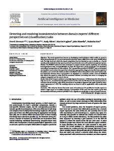
Figure 1: Meta-features values for three address datasets We suggest stratifying the data on the basis of lengths of address records. A longer record can be expected to have greater variation and consist of more structured elements and hence, be more complex for segmentation than a shorter one. Similarly in the case of webpage classification, accuracy on a record (a webpage) would depend on the number of keywords that appear in the webpage. A classifier performing the binary classification would have identified a few important words as the ‘keywords’, that possess greatest predictive power. A webpage having many keywords would be easier to classify than one with fewer number of keywords or the one with no keywords at all. In such a case, we suggest stratifying the dataset on basis of number of words of the webpage identified as key-words. We therefore, adopt the following method for creating a representative sample of size k: 1. Sort the records of the datasets in order of a stratifying criterion 2. Divide the sorted dataset into k equisized bins 3. Randomly select one record from each bin
3.2
Feature Extraction
This section suggests a method of extracting defining features for individual units of the representative samples. Different models can choose a different ‘unit’ of operation according to the task at hand, and also appropriate sets of features for making predictions which depend on the unit. For example, in cases such as address segmentation tasks, the segmentation models tokenize the datasets and extract a set of defining token features for each token, which is the unit of operation. In case of document classification tasks such as that of webpage classification, the unit of operation is records (webpages) and not tokens and features are extracted for the webpages as a whole. Since the task here is predicting the accuracy of model M, and we later use the distribution of the these unit features
Figure 2: Meta-features values for three webpages datasets in estimating the accuracy; we choose a feature set that is same as the feature set used by model M. Unfortunately, this might not always be convenient, specially in segmentation tasks, as some models follow a ‘w-sized window based approach’ to include ‘context’ where the labels of previous w tokens are used as one of the features defining the current token. Since the dataset is unlabeled, we certainly cannot include such features in our design. However, the general idea is to make the two feature sets overlap as much as possible. Following is a list of some features commonly used by classifiers while processing text data such as addresses: relative position of the token in text record, length of the token, capitalization patterns, letter patterns (for example, 2345 and A/2 can be represented as D+ and LSD respectively where D stands for digit, L for letter and S for special characters). In case of several other text processing tasks, such as the document classification task, feature extraction is relatively simpler. The classifier in these cases develops a termdocument matrix. They create a vocabulary of all possible words that appear in the dataset and count of occurrences of the most predictive words of the vocabulary (key-words) is treated as feature vector. Since such a feature vector does not depend on any labels we can easily fulfill the idea of making the two feature sets overlap. Hence, we suggest using the same feature space for accuracy estimation of such classifiers. In Section 4.1.3 we explain further how features can be extracted for such tasks. A representative sample is now expressed as an n1 ×n2 array where, n1 is the total number of units (tokens or records) in the sample and n2 the number of unit features extracted for each unit.
3.3
Meta-feature Creation
The basic idea of estimating the accuracy of a classifier is motivated from the fact that accuracy of any rule based or machine learning model, M can vary considerably from one dataset to another. Had it not been the case, the accuracy of the model on any new data could have been estimated as the accuracy of model on the training set itself. To estimate the accuracy of any model on a new dataset, we need to know
Type of unit feature Continuous Categorical Dictionary based (binary)
Meta-features mean, standard deviation, skewness and kurtosis of individual token features and correlation between unit features taken two at a time entropy fraction of tokens appearing in the concerned dictionary
Table 1: List of meta-features extractable for various types of unit features its accuracy on a few known (possibly small) datasets, and then we would compare the new dataset with these known datasets to get an estimate of accuracy of the model on the new dataset. Therefore, the need for defining the parameters of comparison arises. These parameters are referred to as ‘meta-features’. Since a dataset is composed of units (token/records) and these units are themselves defined by sets of unit features, it is intuitive to compare distribution of these unit features to measure the degree of similarity or dissimilarity between datasets. Therefore, to characterize a representative sample, we refine the statistical and information theoretic measures described in [20] to capture the distributions of the unit features as extracted in previous subsection. Table 1 shows a list of meta-features possible for different types of unit features. Using the meta-features, we thus change the expression of representative sample to an m dimensional vector where m is the total number of meta-features. We subsequently prune the meta-feature set using a stepwise backward elimination procedure described in Section 4. For purpose of visualization, we consider three datasets for address segmentation which were hand tagged by human experts. The datasets exhibited two different accuracies (32.9% for one, considerably different from about 73% for the other two) for a segmentation task using a Conditional Random Field (CRF) [18] based segmentation model. This difference in accuracies can be attributed to differences in the underlying distributions of the datasets. In Figure 1 we show normalized meta-features values for the datasets. There is a considerable difference in almost all the metafeatures values between the two levels of accuracies, whereas the two datasets with similar metafeatures (and hence similar underlying distributions) correspond to roughly the same accuracy. Similarly, we consider three other datasets from a different domain, the webpage classification task. The datasets presented two different accuracy-levels for classification using Support Vector Machine (SVM) [15] based classification model. Figure 2 shows the normalized metafeatures for these datasets. In this case too, there is a similar trend, which corroborates our belief that the meta-features can possibly represent the underlying distribution efficiently, such that any difference (or similarity) in the distribution and hence accuracy, gets reflected in the meta-features values.
3.4
Accuracy Prediction model
We now train a model to learn the accuracy values using the selected meta-features as the predictive variables. For this purpose, we learn a regression model on a metadataset. A meta-dataset is a two dimensional array where samples (datasets) form the rows and the meta-features form columns. The accuracy on a sample is taken as the dependent variable as a function of the meta-features. The accu-
racy estimation model approximates this function in form of a non-linear regression task using SVMs. The training is performed using a few labeled datasets on which the accuracies of the model M are known beforehand. Once an accuracy prediction model has been properly trained, we provide the meta-features of the new representative samples as input to this prediction model and obtain the predicted accuracy.
3.5
Combining sample accuracies
The accuracy of model M on the complete dataset can simply be estimated as the accuracy on any one representative sample. However, for a reliable estimate, one would want to consider the accuracies on several representative samples. We, therefore, draw N different representative samples of same size, estimate the accuracy on each one of them and then combine them to get the accuracy on complete dataset. We also estimate the standard error in this measurement using these N values. Accuracy on a sample is defined as: No. of correctly labeled units Accuracy = Total no. of units in the sample In cases where a record behaves as the ‘unit’ of operation, such as the document classification tasks, the method of choosing representative samples ensures that all the N representative samples will consist of equal number of ‘units’. Hence, the combined accuracy of all samples can be estimated as the mean accuracy of the N representative samples. The combined accuracy of the multiple samples is calculated as follows: 1. Draw N independent equisized representative samples from the complete dataset and use the trained accuracy prediction model to estimate accuracy on each one of them. 2. Estimate the overall accuracy, A as: PN A=
i=1
ai
N
where, ai = Predicted accuracy on sample i. 3. The standard error, δ, in measurement of A can be estimated as the standard deviation of these N accuracy values as follows: s PN 2 i=1 (ai − A) δ= N However, often, the unit of operation in text processing domain is a single token of the record and not the complete record. Since the number of tokens in any record is variable and the method of selecting representative samples operates in a fashion so as to have equal number of records in equisized representative samples, total number of units in the
equisized representative samples will be variable. Therefore, referring to above mentioned definition of accuracy, we cannot accurately estimate the combined accuracy of all samples as the mean accuracy of N representative samples. We, therefore, adopt the following procedure: 1. Independently extract N equisized representative samples from the complete dataset and estimate the accuracy on each of them using the accuracy prediction model. 2. For a representative sample i, define xi such that: xi = Predicted accuracy on sample i × yi where, yi = Total no. of tokens in the sample i. Hence, xi is the estimated number of correctly labeled tokens in sample i. 3. The overall accuracy (A) is defined as: PN xi A = Pi=1 N i=1 yi 4. We estimate the standard error in measurement of A as the standard deviation of the N accuracy values. Since, A is ratio of summations over two variables, its standard q deviation is defined as [12]: σ2
σ2
c
δ = √1N xy¯¯ x¯x2 + y¯y2 − 2 x¯xy y ¯ where, x ¯, y¯= mean values of x and y respectively σx , σy = standard deviation of x and y respectively cxy =covariance of x and y
Finally, the estimated accuracy of model M on the complete dataset is [5]: A ± (zδ) where, z determines the confidence interval assuming a normal distribution of the samples’ accuracies. For 90%, 95% and 99% confidence intervals, the corresponding z values are 1.65, 1.96 and 2.58 respectively. The expression (zδ) is called the margin of error (E). Choosing the appropriate value of N : In this approach, one also needs to decide the number of representative samples required for obtaining a desired margin of error, E. Now, E = zδ Alternatively, φ E = z√ N where, φ=
x ¯ y¯
s
σy2 σx2 cxy + 2 −2 2 x ¯ y¯ x ¯y¯
Therefore, zφ 2 ) E Unfortunately, to determine the value of N we need to have a separate estimate of φ besides z and E. The value of z N =(
and E can be set as desired by the user while the value of φ is estimated from a pilot study. A pilot study is a small experiment aimed at obtaining a rough estimate of some variable (φ in our case). We propose to draw n (say, 50) representative samples from the dataset and calculate φ for this set of samples using the formula mentioned above. Since, the value of φ does not vary considerably with different values of N , this value can hence be used as a rough estimate of φ. The appropriate value of N for a desired margin of error can now be estimated using the formula.
4.
EXPERIMENTS AND RESULTS
The major constraint in the study is a lack of large sized labeled textual data for robust testing of the complete system at one go. We, therefore, divide the evaluation into two separate phases for validating the accuracy prediction model and the sampling method. We use a heterogeneous set of several small sized labeled datasets with manually computed accuracies for testing the accuracy prediction model. For the sampling method, it suffices to show that estimated accuracy on the entire dataset using the sampling method is the same as the estimate predicted by running the accuracy prediction model for the entire dataset itself. Additionally, we manually annotate a smaller subset of the huge dataset; calculate accuracy of the model on this subset and compare its value with the predicted value.
4.1
The Accuracy Prediction Model
We designed and tested accuracy prediction models for three different classifiers. 1. A CRF model for segmenting Indian postal addresses 2. A rule based model for segmenting Indian postal addresses 3. An SVM classifier for classifying text of webpages as faculty/student webpage In each case, the accuracy prediction model was built and tested on labeled datasets. We used Support Vector Machine for regression [19] on accuracies of datasets. Evaluation Criterion: We used Mean Absolute Error (MAE) to measure the performance of our accuracy prediction model on a test set consisting of, say, n datasets. It is defined as: M AE =
1 n
Pn
i=1
|fi − yi |
Here fi is the estimated accuracy for dataset i and yi is the actual accuracy. Evaluation Methodology: In our experiments, we often use Leave-one-out (LOO) Cross Validation to compute MAE. LOO-Cross Validation is a popular validation technique for predictive models where one of the data points is treated as the validation point and the model is trained on the remaining point. The performance of the model on the validation set is compared to the known results. The process is repeated till each data point is used once as validation set. For our experiments, the accuracy prediction model is the predictive model and the various labeled datasets behave as the data points.
Dataset number 1-14 15-16 17-19
Description
Mumbai addresses Delhi addresses All states addresses
No. of datasets 14
No. of records in each dataset 50
2
50
2
3
50
3
Table 2: Datasets for validating the Accuracy Prediction model (using CRF)
In a few cases, we use hold-out validation where we mark a few labeled datasets (which are known to be mutually similar, but different from others) as the validation set and train the accuracy prediction model on the other datasets. The predictions made by the accuracy prediction model on the validation set are compared to the actual values.
4.1.1
Exp. No. 1
Experiment Name Accuracy estimation of CRF Accuracy estimation of Rule Based model Accuracy estimation of SVM
1. Token length: numeric 2. Relative position of the token in address record: numeric 3. Type of characters in the token (alphanumeric/ alldigits/all-letters): categorical 4. Presence of the token in the training dictionary: binary Meta-features creation and selection: We extract meta-features as described in Table 1. Todorovski et al. [20] point out that an optimal meta-feature set should be chosen for best performance of a meta-learner. In our experiments, we selected an optimal meta-feature subset by stepwise backward elimination using LOO-Cross Validation on the meta-dataset consisting of training examples. Table 3 shows that selection of an optimal subset indeed leads to a better accuracy prediction model which has a lower MAE for LOO-Cross Validation.
2.92
2.04
4.32
1.49
Table 3: Effect of meta-feature selection on performance of the accuracy prediction model Token feature Token length
Token position
Estimating Accuracy of the CRF
Datasets: We used labeled address datasets from various Indian geographies for this experiment. A brief description of the datasets is provided in Table 2. Classifier: We designed an accuracy prediction model to estimate the accuracy of a CRF based segmentation model [16, 17, 18]. The CRF was trained on one of the Mumbai datasets of 50 records, tested on all the 19 datasets and accuracies of the trained CRF were noted for each of the 19 datasets. Feature extraction: The CRF model tokenizes the textual address dataset and extracts various features for each token. It then creates a ‘Training dictionary’ which is a dictionary of lexical entities appearing in the training dataset and then checks for appearances of those words at specific locations in the test record, looking for previous labels at the same time. It also checks for the letter patterns in the tokens apart from token’s position and length. To make the feature set overlap as much as possible with the feature set used by the CRF model, we use the following features:
MAE for LOO-Cross Validation Before After 3.90 3.13
Symbol type Presence in dictionary
Meta-feature Mean Standard deviation Skewness Kurtosis Mean Standard deviation Skewness Kurtosis Entropy Fraction of tokens
Correlation 0.0474 0.1764 0.107 0.1177 0.2804 0.3163 0.4335 0.3451 0.4978 0.8943
Table 4: Spearman rank Correlation values of metafeatures values and accuracy values
Since we estimate a model’s accuracy using meta-features, it is essential for the meta-features to have good predictive potential. A measure of correlation between the metafeatures values and the accuracy values might yield insights into capabilities of the meta-features. Table 4 shows the extent of non linear correlation between the meta-features and the accuracy values. The table shows that a few metafeatures have fair correlation with the accuracy values, particularly one based on fraction of tokens appearing in training dictionary. It also suggests that mean length of tokens, which has a low correlation with accuracy, might not be a powerful meta-feature. This is corroborated when we drop this meta-feature during the meta-feature subset selection phase. Validating the model: We tested our accuracy prediction model using LOO-Cross Validation and obtained a mean absolute error of 3.13. However, we believe that LOOCross Validation would not be the best evaluation strategy in this case because there are more than one datasets belonging to one geographical location and a model trained on addresses of a particular geographical location is expected to perform well in predicting accuracy on addresses of the same location as it had learnt similar addresses during training. We, therefore, carried out two different hold out validation experiments for a more robust testing in which the training and validation sets were from different geographical locations. The detailed results are presented in Table 5.
Training datasets No 1-16
Validation dataset No. 17-19
1-14,17-19
15-16
(Actual Accuracy, Estimated Accuracy) (49.37%,48.18%) (46.55%,52.54%) (28.02%,28.78%) (35.68%,33.67%) (32.97%,37.79%)
MAE 2.65 3.42
Table 5: Results of validation of the accuracy prediction model (using CRF) for address segmentation (Dataset numbers as mentioned in Table 2)
4.1.2
Estimating Accuracy of the Rule Based Classifier
Datasets: In this experiment, we use 21 labeled address datasets from more than 11 different Indian states. Each dataset contains 100 address records. Classifier: We validate our technique for estimating accuracy of a Rule based segmentation model. The model was designed by domain experts who manually constructed a rule base comprising of about a thousand rules. For the experiment, we ran the model on the 21 datasets, and noted its accuracy on each of them. Features extraction: This classifier relied on use of dictionaries of various Indian states, Cities and Postal codes, letter patterns, location of a token in an address etc. Apart from maintaining dictionary, the model looked for patterns and positioning of the tokens. Thus, the token features described in Section 4.1.1 would also be sufficient for this task. Meta-features creation and selection: We extract the same meta-features as described in Table 1 and used stepwise backward elimination using LOO-Cross Validation for selecting the optimal subset. The effect of meta-feature subset selection on model’s performance is shown in Table 3. Validating the model: We tested our prediction model using LOO-Cross Validation and obtained a mean absolute error of 2.04. Also, as before, for more realistic testing, we carried out hold-out validation where we ensured that the validation and training set contain datasets from different geographies. Results are summarized in Table 6.
ture space in this case was large (22 dimensional). Hence, we had to be careful about deciding the meta-features to be extracted so as to best capture their distribution with minimum number of meta-features. Owing to the sparse nature of the term-document matrix, the features (count of occurrences of terms) were zero for most of the webpage instances. We, therefore, derived the following meta-features for each feature and used stepwise backward elimination for selecting the optimal subset. 1. Mean of the unit feature: Mean number of occurrences of a term 2. Degree of sparseness of the unit feature: Number of times the term occurred at least once in the dataset Table 3 highlights the benefits of choosing optimal subset in terms of an improved Mean Absolute Error. Validating the model: In this experiment too, LOOCross Validation was used for testing the prediction model, and we achieved a mean absolute error of 1.49. We provide detailed results for few of the 30 testsets in Table 7
4.1.4
Since, in our case, all the validation and training datasets were of equal size, we could not explore ‘size of dataset’ as one of the meta-features. One needs to be careful, however, while using the accuracy prediction model on a larger dataset as absence of this meta-feature might lead to incorrect estimation.
4.2 4.1.3
Estimating Accuracy of the SVM
Datasets: We used ‘The 4 Universities’ dataset [1] collected by the CMU text learning group. The dataset contains WWW-pages collected from Computer Science departments of various universities. We use a subset of the data containing only faculty and student webpages and divided this into 30 equisized parts, so that each part could be treated as an independent dataset. Classifier: We designed a binary SVM based classifier for classifying a webpage as a faculty or a student webpage. One of the 30 parts was chosen as the training set and the remaining 29 were used as test sets. The training set was tokenized and a term-document matrix was created. The features, hence represented term occurrences. We then chose an optimal feature subset using the correlation based feature selection technique [9]. The SVM was trained using this feature subset followed by testing on the 29 test sets. The accuracies on each of the testsets were noted for use in the accuracy prediction task. Features extraction: The SVM model was using the count of occurrences of most predictive terms as features. We use the same feature space as the feature set used by the SVM. Meta-features creation and selection: The unit fea-
Dataset Size:
Sampling Method: Accuracy estimation on large unlabeled dataset
Datasets: We used two unlabeled Indian address datasets for validating the sampling technique. The datasets comprised of 123910 and 399786 addresses respectively. The Classifier: We verify the sampling method by predicting accuracy of the Rule based model (described in Section 4.1.2) on the two unlabeled datasets. Validating the method: An ideal validation method would use a labeled dataset, so that actual accuracy on the complete dataset and any representative sample would be known. One could then have used the method described in Section 3.5 to estimate the accuracy on the dataset and compared it with the known accuracy. However, large labeled datasets are unavailable, and hand tagging unlabeled dataset is costly. Hence, we exploit our prediction model designed in Section 4.1.2 to estimate the accuracy on the complete dataset (time-consuming) as well as on the representative samples; and contend that the estimate through sampling is essentially the same as through using the prediction model on the entire huge corpus. The size of representative samples is kept constant at 100 records (same as the size of the datasets used for training the accuracy prediction model) because of reasons explained in Section 4.1.4.
Test datasets description Rajasthan Haryana All states
No. of test datasets 2 2 5
(Actual Accuracy, Estimated Accuracy)
MAE
(93.83%,95.81%) (93.62%,97.03%) (97.10%,92.59%) (97.32%,89.68%) (92.27%,94.43%) (94.07%,94.78%) (91.12%,94.04%) (92.36%,93.40%) (91.96%,94.17%)
2.70 6.08 1.81
Table 6: Results of validation of accuracy prediction model (using Rule based model) for address segmentation Test set number Actual Accuracy Estimated Accuracy Absolute Error
1 95.00% 94.17% 0.83
2 85.00% 86.71% 1.71
3 83.00% 84.03% 1.03
4 91.00% 90.54% 0.46
5 87.00% 85.37% 1.63
Table 7: Results of validation of the accuracy prediction model (using SVM) for webpage classification The complete dataset could not be provided as input to the accuracy prediction model because of its huge size (refer to Section 4.1.4). Therefore, to estimate the accuracy on the complete dataset, we divided the dataset into G equisized groups (of 100 records each) and used the accuracy prediction model to estimate the accuracy on each of these G groups. We then calculate the accuracy on the complete dataset as: PG i=1 xi Accuracy = PG j=1 yj where, yj = Total no. of tokens in group j xi = Predicted accuracy of group i ×yi To keep the evaluation fair, it was ensured that these G groups aren’t a superset of the representative samples used for estimating accuracy. Additionally, for one of the datasets (consisting of 123910 records), a randomly chosen subset of size 1000 records was hand tagged by human experts and the actual accuracy value computed (assuming that the accuracy on the complete dataset will be close to the accuracy obtained on this sample). This value was then compared with the estimated values. For each of the two unlabeled datasets, we then compared the accuracy as estimated by our sampling method with the accuracy as predicted by prediction model and that obtained by hand tagging. Table 8 shows that in both the cases, the accuracies estimated by sampling method are fairly close to the actual values. Comparison with Simple Random Sampling: We compare our method with Simple Random Sampling wherein we follow a procedure similar to one described in Section 3.5. The only difference lies in the way samples are created. In this case, a sample is created by Simple Random Sampling [21] instead of a binning procedure, and selecting one record from each bin. Table 8 shows that while both the sampling methods lead to an overall estimated accuracy close to the actual value, Simple Random Sampling leads to a greater Margin of Error (zδ). This happens because some of the samples selected by this method are not sufficiently representative of the dataset and hence have an accuracy considerably different from the overall accuracy, A which results in a larger value of standard error (δ).
5.
DISCUSSION AND CONCLUSION
In this study we investigate the use of meta-learning for predicting the accuracy of a classifier designed to process text data. The method involves extracting a descriptive feature set for each token of the free text data and then capturing their distribution via the meta-features. Thus, the metafeatures are essentially measures to characterize a dataset. This is followed by estimating the accuracy by an SVM based accuracy prediction model which is trained on accuracies of labeled datasets. This prediction model building procedure, though requires some labeling of small datasets for training, is a one-time involvement. Once a model has been built, it can be used repeatedly on new datasets without putting in additional effort. We validate our method for three different types of classifiers and show that the estimated accuracies are close to the actual values. Additionally, we demonstrate that the meta-features we use are correlated with accuracy. We also suggest and validate a sampling method using binning to effectively choose representative samples from a huge dataset that are better than simple random samples, and use it for efficient accuracy estimation on the dataset. Our sampling method helps us in avoiding large computational overheads without affecting the performance of the accuracy prediction model. We empirically show that the accuracy of complete dataset lies within the bounds we estimate from its representative samples. Our experiments also suggest that the samples drawn using our method are more representative than the samples drawn using Simple Random Sampling. This method of estimation of accuracies can be developed as a possible active learning approach and be used for selecting an appropriate training set. Building a model essentially requires labeled training set. However, for huge datasets, a training set is only a sample of the whole dataset. It is necessary to ensure that the training set is representative so that the model scales to the full dataset. Also, when developing a model, the accuracy of model on different subsets of the data can vary greatly. The proposed method can be used to identify those subsets that give low accuracy, which can be labeled and then used in training. In this way, the model can be scaled up quickly, by appropriately selecting training data, to have better accuracy on the entire dataset. Due to insufficient data, we could not explore the role of dataset size as one of the potential meta-features. Future work can explore this possibility.
Sl No.
Number Actual Estimated of Accuracy1 Accuracy2 records Representative Sampling: 1 123910 84.84% 84.15% 2 399786 – 73.68% Simple Random Sampling: 1 123910 84.84% 84.44% 2 399786 – 73.31% 1 On
a subset of 1000 records
2 On
Accuracy as estimated by samples3 Set1 Set2 N A ± zδ N A ± zδ 50 50
84.13±1.30% 74.81±1.19%
100 100
84.16±1.32% 73.37±1.43%
50 50
84.54±3.89% 73.50±2.80%
100 100
84.48±2.95% 73.44±3.12%
complete dataset
3 95%
confidence limit
Table 8: Results of experiments on the Sampling Method for accuracy estimation of a Rule based model for address segmentation (N =Number of representative samples drawn from the dataset)
6.
REFERENCES
[1] http://www.cs.cmu.edu/afs/cs.cmu.edu/project/theo20/www/data. [2] H. Bensusan and A. Kalousis. Estimating the predictive accuracy of a classifier. In Proceedings of EMCL ’01, pages 25–36, London, UK, 2001. Springer-Verlag. [3] O. Chapelle, B. Sch¨ olkopf, and A. Zien. Semi-Supervised Learning. MIT Press, 2006. [4] D. A. Cieslak and N. V. Chawla. Detecting fractures in classifier performance. In Proceedings of ICDM ’07, pages 123–132, Washington, DC, USA, 2007. IEEE Computer Society. [5] W. G. Cochran, editor. Sampling Techniques, 3rd Edition. John Wiley, 1977. [6] D. Cohn, R. Ladner, and A. Waibel. Improving generalization with active learning. In Machine Learning, pages 201–221, 1994. [7] C. B. Do and A. Y. Ng. Transfer learning for text classification. In NIPS, 2005. [8] T. A. Faruquie, K. H. Prasad, L. V. Subramaniam, M. K. Mohania, G. Venkatachaliah, S. Kulkarni, and P. Basu. Data cleansing as a transient service. In ICDE, pages 1025–1036, 2010. [9] M. A. Hall. Correlation-based feature subset selection for machine learning. Hamilton, New Zealand, 1999. [10] A. Kalousis and T. Theoharis. Noemon: Design, implementation and performance results of an intelligent assistant for classifier selection. Intelligent Data Analysis, 3(5):319–337, 1999. [11] G. Kothari, T. A. Faruquie, L. V. Subramaniam, K. H. Prasad, and M. K. Mohania. Transfer of supervision for improved address standardization. In Proceedings of ICPR ’10, 2010. [12] H. Ku. Notes on the use of propagation of error formulas. J Research of National Bureau of Standards-C. Engineering and Instrumentation, 70C(4):263–273, 1966. [13] D. Michie, D. J. Spiegelhalter, C. C. Taylor, and J. Campbell, editors. Machine learning, neural and statistical classification. Ellis Horwood, Upper Saddle River, NJ, USA, 1994. [14] B. Pfahringer, H. Bensusan, and C. G. Giraud-Carrier. Meta-learning by landmarking various learning algorithms. In Proceedings of ICML ’00, pages 743–750, San Francisco, CA, USA, 2000. Morgan Kaufmann Publishers Inc.
[15] J. Platt. Machines using sequential minimal optimization. In B. Schoelkopf and C. Burges and A. Smola, editors, Advances in Kernel Methods - Support Vector Learning. MIT Press, 1998. [16] S. Sarawagi. Efficient inference on sequence segmentation models. In Proceedings of ICML ’06, 2006. [17] S. Sarawagi and W. W. Cohen. Semi-markov conditional random fields for information extraction. In NIPS, 2004. [18] F. Sha and F. Pereira. Shallow parsing with conditional random fields. In Proceedings of HLT-NAACL, 2003. [19] A. J. Smola and B. Schoelkopf. A tutorial on support vector regression. NeuroCOLT2 Technical Report Series, 1998. [20] L. Todorovski, P. Brazdil, and C. Soares. Report on the experiments with feature selection in meta-level learning. In Proceedings of the Workshop on Data Mining, Decision Support, Meta-learning and ILP at PKDD’2000, pages 27–39, 2000. [21] D. S. Yates, D. S. Moore, and D. S. Starnes, editors. The Practice of Statistics, 3rd Edition. Freeman, 2008.