Vitaly Schetinin, Jonathan E. Fieldsend, Derek Partridge, Wojtek J. Krzanowski, Richard M. ...... Stanford, CA: Morgan Kaufmann, pp. 223-230. 10.Schetinin V ...
Estimating Classification Uncertainty of Bayesian Decision Tree Technique on Financial Data Vitaly Schetinin, Jonathan E. Fieldsend, Derek Partridge, Wojtek J. Krzanowski, Richard M. Everson, Trevor C. Bailey and Adolfo Hernandez School of Engineering, Computer Science and Mathematics, University of Exeter, EX4 4QF, UK
Emails: {v.schetinin, j.e.fieldsend, d.partridge, w.j.krzanowski, r.m.everson, t.c.bailey, a.hernandez}@exeter.ac.uk
Abstract. Bayesian averaging over classification models allows the uncertainty of classification outcomes to be evaluated, which is of crucial importance for making reliable decisions in applications such as financial in which risks have to be estimated. The uncertainty of classification is determined by a trade-off between the amount of data available for training, the diversity of a classifier ensemble and the required performance. The interpretability of classification models can also give useful information for experts responsible for making reliable classifications. For this reason Decision Trees (DTs) seem to be attractive classification models. The required diversity of the DT ensemble can be achieved by using the Bayesian model averaging all possible DTs. In practice, the Bayesian approach can be implemented on the base of a Markov Chain Monte Carlo (MCMC) technique of random sampling from the posterior distribution. For sampling large DTs, the MCMC method is extended by Reversible Jump technique which allows inducing DTs under given priors. For the case when the prior information on the DT size is unavailable, the sweeping technique defining the prior implicitly reveals a better performance. Within this Chapter we explore the classification uncertainty of the Bayesian MCMC techniques on some datasets from the StatLog Repository and real financial data. The classification uncertainty is compared within an Uncertainty Envelope technique dealing with the class posterior distribution and a given confidence probability. This technique provides realistic estimates of the classification uncertainty which can be easily interpreted in statistical terms with the aim of risk evaluation.
2 Vitaly Schetinin, Jonathan E. Fieldsend, Derek Partridge, Wojtek J. Krzanowski, Richard M. Everson, Trevor C. Bailey and Adolfo Hernandez
1.
Introduction
The uncertainty of Bayesian model averaging used for applications such as financial prediction in which risks should be evaluated is of crucial importance. In general, uncertainty is a triple trade-off between the amount of data available for training, the classifier diversity and the classification accuracy [1 - 4]. The interpretability of classification models can also give useful information to experts responsible for making reliable classifications. For this reason Decision Trees (DTs) seem to be attractive classification models for experts [1 - 7]. The main idea of using DT classification models is to recursively partition data points in an axis-parallel manner. Such models provide natural feature selection and uncover the features which make the important contribution the classification. The resultant DT classification models can be easily interpretable by users. By definition, DTs consist of splitting and terminal nodes, which are also known as tree leaves. DTs are said to be binary if the splitting nodes ask a specific question and then divide the data points into two disjoint subsets, say the left or the right branch. Fig. 1 depicts an example of the DT consisting of two splitting and three terminal nodes. Q1 Yes
No Q2
P1
Yes
No
P2
P3
Fig. 1. An example of decision tree consisting of two splitting and terminal nodes depicted by the circles and rectangles. The split nodes ask the questions Q1 and Q2 and an outcome is assigned to one of the terminal nodes with the probabilities P1, P2, and P3.
Note that the number of the data points in each split should not be less than that predefined by a user. The terminal node assigns all data points falling in that node to a class of majority of the training data points resid-
Estimating Classification Uncertainty of Bayesian Decision Tree Technique on Financial Data 3
ing in this terminal node. Within a Bayesian framework, the class posterior distribution is calculated for each terminal node [4 - 7]. The required diversity of the DTs can be achieved on the base of Bayesian Markov Chain Monte Carlo (MCMC) methodology of sampling from the posterior distribution [4 - 7]. This technique has revealed promising results when applied to some real-world problems. Chipman et al. [6] and recently Denison et al. [7] have suggested the MCMC techniques in which for sampling from large DTs they used Reversible Jumps (RJ) extension suggested by Green [8]. The RJ MCMC technique making such moves as birth and death allows the DTs to be induced under the priors given on the shape or size of the DTs. Exploring the posterior distribution, the RJ MCMC should keep the balance between the birth and death moves under which the desired estimate of the posterior can be unbiased [6 - 8]. Within the RJ MCMC technique the proposed moves for which the number of data points falling in one of splitting nodes becomes less than the given number are assigned unavailable. Obviously that the priors given on the DTs are dependent on the class boundaries and noise level in data available for training, and it is intuitively clear that the sharper class boundaries, the larger DTs should be. However in practice the use of such an intuition without a prior knowledge on favourite shape of the DTs can lead to inducing over-complicated DTs and as a result the averaging over such DTs can produce biased class posterior estimates [6, 7]. More over, within the standard RJ MCMC technique suggested for averaging over DTs, the required balance cannot be kept. This may happen because of over-fitting the Bayesian DTs [9]. Another reason is that the RJ MCMC technique averaging over DTs assigns some moves which can not provide a given number of data points allowed being in the splitting nodes unavailable [10]. For the cases when the prior information of the favourite shape of DTs is unavailable, the Bayesian DT technique with a sweeping strategy has revealed a better performance [10]. Within this strategy the prior given on the number of DT nodes is defined implicitly and dependent on the given number of data points allowed being at the DT splits. So the sweeping strategy gives more chances to induce the DTs containing a near optimal number of splitting nodes required to provide the best generalization. At the same time within this technique the number of data points allowed to be in the splitting nodes can be reasonably reduced without increasing the risk of overcomplicating the DTs. In this Chapter we compare the classification uncertainty of the Bayesian DT techniques with the standard and sweeping RJ MCMC strategies on a synthetic dataset as well on the real financial datasets known as the Aus-
4 Vitaly Schetinin, Jonathan E. Fieldsend, Derek Partridge, Wojtek J. Krzanowski, Richard M. Everson, Trevor C. Bailey and Adolfo Hernandez
tralian and German Credit datasets from the StatLog Repository [11]. In our experiments we also used the Company Liquidity Data recently announced by the German Classification Society for competition in data mining [12]. The classification uncertainty of the Bayesian techniques is evaluated within an Uncertainty Envelope dealing with the class posterior distribution and a given confidence probability suggested in [13]. The Uncertainty Envelope technique by estimating the consistency of DT outputs on the given data produces allows the classification uncertainty to be estimated and interpreted in statistical terms [14]. Using such an evaluation technique in our comparative experiments, we find that the Bayesian DT technique with the sweeping strategy is superior to the standard RJ MCMC technique. In section 2 we first describe the standard Bayesian RJ MCMC technique and then in section 3 we describe the Bayesian DT technique with the sweeping strategy. In section 4 we briefly describe the Uncertainty Envelope technique used in our experiments for comparison of the classification uncertainty of the two Bayesian DT techniques. The experimental results are presented in section 5, and section 6 concludes the Chapter.
2.
The Bayesian Decision Tree Technique
In this section we first present the Bayesian DT technique based on MCMC search methodology and second describe Reversible Jump extension of the MCMC. Finally we discuss the difficulties of sampling large DTs within the RJ MCMC technique. 2.1. The Bayesian Averaging over Decision Trees In general, the predictive distribution we are interested in is written as an integral over parameters θ of the classification model p ( y | x, D) = p ( y | x, , D) p ( | D)d
(1)
θ
where y is the predicted class (1, …, C), x = (x1, …, xm) is the mdimensional input vector, and D denotes the given training data. The integral (1) can be analytically calculated only in simple cases. In practice, part of the integrand in (1), which is the posterior density of θ conditioned on the data D, p(θ θ | D), cannot usually be evaluated. However
Estimating Classification Uncertainty of Bayesian Decision Tree Technique on Financial Data 5
if values θ (1), …, θ (N) are drawn from the posterior distribution p(θ θ | D), we can write p ( y | x, D) ≈
N
p ( y | x,
(i )
i =1
, D) p (
(i)
| D) =
1 N
N
p ( y | x,
(i )
, D) .
(2)
i =1
This is the basis of the MCMC technique for approximating integrals [7]. To perform the approximation, we need to generate random samples from p(θ θ | D) by running a Markov Chain until it has converged to a stationary distribution. After this we can draw samples from this Markov Chain and calculate the predictive posterior density (2). Let us now define a classification problem presented by data (xi, yi), i = 1, …, n, where n is the number of data points and yi ∈ {1, …, C} is a categorical response. Using DTs for classification, we need to determine the probability ϕij with which a datum x is assigned by terminal node i = 1, …, k to the jth class, where k is the number of terminal nodes in the DT. Initially we can assign a (C – 1)-dimensional Dirichlet prior for each terminal node so that p(ϕ ϕi | θ) = DiC-1(ϕ ϕi | α), where ϕi = (ϕi1, …, ϕiC), θ is the vector of DT parameters, and α = (α1, …, αC) is a prior vector of constants given for all the classes. The DT parameters are defined as θ = (sipos, sivar, sirule), i = 1, …, k – 1, where sipos, sivar and sirule define the position, predictor and rule of each splitting node, respectively. For these parameters the priors can be specified as follows. First we can define a maximal number of splitting nodes, say, smax = n – 1, so sipos ∈ {1,..., s max } . Second we draw any of the m predictors from a uniform discrete distribution U(1, …, m) and assign var s ivar ∈ {1,..., m} . Finally the candidate value for the splitting variable xj = si is drawn from a uniform discrete distribution U(xj(1), …, xj(N)), where N is the total number of possible splitting rules for predictor xj, either categorical or continuous. Such priors allow the exploring of DTs which partition data in as many ways as possible, and therefore we can assume that each DT with the same number of terminal nodes is equally likely [7]. For this case the prior for a complete DT is described as follows: p( ) =
k −1
∏ p(s i =1
rule i
| sivar ) p ( sivar ) p ({sipos }1k −1 ).
(3)
For a case when there is knowledge of the favoured structure of the DT, Chipman et al. [6] suggested a generalisation of the above prior – they as-
6 Vitaly Schetinin, Jonathan E. Fieldsend, Derek Partridge, Wojtek J. Krzanowski, Richard M. Everson, Trevor C. Bailey and Adolfo Hernandez
sume the prior probability of further split of the terminal nodes to be dependent on how many splits have already been made above them. For example, for the ith terminal node the probability of its splitting is written as (4)
p split (i ) = γ (1 + d i ) −δ ,
where di is the number of splits made above i and γ, δ ≥ 0 are given constants. The larger δ, the more the prior favours “bushy” trees. For δ = 0 each DT with the same number of terminal nodes appears with the same prior probability. Having set the priors on the parameters ϕ and θ, we can determine the marginal likelihood for the data given the classification tree. In the general case this likelihood can be written as a multinomial Dirichlet distribution [7]: Γ{αC} p(D | ) = {Γ (α )}C
k
C
∏
C
∏ Γ (n i =1
j i
Γ (mij + α j ) +
C
α j) j =1
,
(5)
where ni is the number of data points falling in the ith terminal node of which mij points are of class j and Γ is a Gamma function. 2.2 Reversible Jumps Extension To allow sampling DT models of variable dimensionality, the MCMC technique exploits the Reversible Jump extension [8]. This extension allows the MCMC technique to sample large DTs induced from real-world data. To implement the RJ MCMC technique Chipman et al. [6] and Denison et al. [7] have suggested exploring the posterior probability by using the following types of moves. • Birth. Randomly split the data points falling in one of the terminal nodes by a new splitting node with the variable and rule drawn from the corresponding priors. • Death. Randomly pick a splitting node with two terminal nodes and assign it to be one terminal with the united data points. • Change-split. Randomly pick a splitting node and assign it a new splitting variable and rule drawn from the corresponding priors. • Change-rule. Randomly pick a splitting node and assign it a new rule drawn from a given prior.
Estimating Classification Uncertainty of Bayesian Decision Tree Technique on Financial Data 7
The first two moves, birth and death, are reversible and change the dimensionality of θ as described in [7]. The remaining moves provide jumps within the current dimensionality of θ. Note that the change-split move is included to make “large” jumps which potentially increase the chance of sampling from a maximal posterior whilst the change-rule move does “local” jumps. For the birth moves, the proposal ratio R is written R=
q( | ' ) p( ' ) , q( ' | ) p( )
(6)
where the q( | ' ) and q( ' | ) are the proposed distributions, θ´ and θ are (k + 1) and k-dimensional vectors of DT parameters, respectively, and p(θ θ) and p(θ θ´) are the probabilities of the DT with parameters θ and θ´: k −1
p( ) = {∏ i =1
1 1 k 1, } N ( sivar ) m S k K
(7)
where N ( s ivar ) is the number of possible values of sivar which can be assigned as a new splitting rule, Sk is the number of ways of constructing a DT with k terminal nodes, and K is the maximal number of terminal nodes, K = n – 1. For binary DTs, as given from graph theory, the number Sk is the Catalan number Sk =
1 2k , k +1 k
(8)
and we can see that for k ≥ 25 this number becomes astronomically large, Sk ≥ (4.8)12. The proposal distributions are as follows q( | ' ) =
q( ' | ) =
d k +1 , DQ '
bk 1 1 , k N ( skvar ) m
(9) (10)
where DQ1 = DQ + 1 is the number of splitting nodes whose branches are both terminal nodes. Then the proposal ratio for a birth is given by
8 Vitaly Schetinin, Jonathan E. Fieldsend, Derek Partridge, Wojtek J. Krzanowski, Richard M. Everson, Trevor C. Bailey and Adolfo Hernandez
R=
d k +1 k S k . bk DQ1 S k +1
(11)
The number DQ1 in (11) is dependent on the DT structure and it is clear that DQ1 < k ∀ k = 1, …, K. Analysing (11), we can also assume dk+1 = bk. Then letting the DTs grow, i.e., k → K, and considering Sk+1 > Sk, we can see that the value of R → c, where c is a constant lying between 0 and 1. Alternatively, for the death moves the proposal ratio is written as R=
bk DQ S k , d k −1 (k − 1) S k −1
(12)
and we can see that under the assumptions considered for the birth moves, R ≥ 1. 2.3. The Difficulties of Sampling Decision Trees The RJ MCMC technique starts drawing samples from a DT consisting of one splitting node whose parameters were randomly assigned within the predefined priors. So we need to run the Markov Chain while it grows and its likelihood is unstable. This phase is said burn-in and it should be preset enough long in order to stabilize the Markov Chain. When the Markov Chain will be enough stable, we can start sampling. This phase is said post burn-in. It is important to note that the DTs grow very quickly during the first burn-in samples. This happens because an increase in log likelihood value for the birth moves is much larger than that for the others. For this reason almost every new partition of data is accepted. Once a DT has grown the change moves are accepted with a very small probability and, as a result, the MCMC algorithm tends to get stuck at a particular DT structure instead of exploring all possible structures. The size of DTs can rationally decrease by defining a minimal number of data points, pmin, allowed to be in the splitting nodes [3 - 5]. If the number of data points in new partitions made after the birth or change moves becomes less than a given number pmin, such moves are assigned unavailable, and the RJ MCMC algorithm resamples such moves. However, when the moves are assigned unavailable, this distorts the proposal probabilities pb, pd, and pc given for the birth, death, and change moves, respectively. The larger the DT, the smaller the number of data
Estimating Classification Uncertainty of Bayesian Decision Tree Technique on Financial Data 9
points falling in the splitting nodes, and correspondingly the larger is the probability with which moves become unavailable. Resampling the unavailable moves makes the balance between the proposal probabilities biased. To show that the balance of proposal probabilities can be biased, let us assume an example with probabilities pb, pd, and pc set equal to 0.2, 0.2, and 0.6, respectively, note that pb + pd + pc = 1. Let the DTs be large so that the birth and change moves are assigned unavailable with probabilities pbu and pcu equal to 0.1 and 0.3, respectively. As a result, the birth and change moves are made with probabilities equal to (pb – pbu) and (pc – pcu), respectively. Let us now emulate 10000 moves with the given proposal probabilities. The resultant probabilities are shown in Fig. 2.
Fig. 2. The standard strategy: The proposal probabilities for the birth, death and change moves presented by the three groups. The left hand bars in each group denote the proposal probabilities. The right hand bars denote the resultant probabilities with which the birth, death, and change moves are made in reality if the birth and change moves were assigned unavailable with probabilities 0.1 and 0.3, respectively.
From the above figure we can see that after resampling the unavailable proposals the probabilities of the birth and death moves become equal ap-
10 Vitaly Schetinin, Jonathan E. Fieldsend, Derek Partridge, Wojtek J. Krzanowski, Richard M. Everson, Trevor C. Bailey and Adolfo Hernandez
proximately 0.17 and 0.32, i.e., the death moves are made with a probability which is significantly larger than a probability originally set equal 0.2. The disproportion in the balance between the probabilities of birth and death moves is dependent on the size of DTs averaged over samples. Clearly, at the beginning of burn-in phase the disproportion is close to zero, and to the end of the burn-in phase, when the size and form of DTs are stabilized, its value becomes maximal. Because DTs are hierarchical structures, the changes at the nodes located at the upper levels can significantly change the location of data points at the lower levels. For this reason there is a very small probability of changing and then accepting a DT split located near a root node. Therefore the RJ MCMC algorithm collects the DTs in which the splitting nodes located far from a root node were changed. These nodes typically contain small numbers of data points. Subsequently, the value of log likelihood is not changed much, and such moves are frequently accepted. As a result, the RJ MCMC algorithm cannot explore a full posterior distribution properly. One way to extend the search space is to restrict DT sizes during a given number of the first burn-in samples as described in [7]. Indeed, under such a restriction, this strategy gives more chances of finding DTs of a smaller size which could be competitive in term of the log likelihood values with the larger DTs. The restricting strategy, however, requires setting up in an ad hoc manner the additional parameters such as the size of DTs and the number of the first burn-in samples. Sadly, in practice, it often happens that after the limitation period the DTs grow quickly again and this strategy does not improve the performance. Alternatively to the above approach based on the explicit limitation of DT size, the search space can be extended by using a restarting strategy as Chipman et al. have suggested in [6]. Clearly, both these strategies cannot guarantee that most of DTs will be sampled from a model space region with a maximal posterior. In the next section we describe our approach based on sweeping the DTs. 3. The Bayesian Averaging with a Sweeping Strategy In this section we describe our approach to decreasing the uncertainty of classification outcomes within the Bayesian averaging over DT models. The main idea of this approach is to assign the prior probability of further splitting DT nodes to be dependent on the range of values within which the number of data points will be not less than a given number of points, pmin.
Estimating Classification Uncertainty of Bayesian Decision Tree Technique on Financial Data 11
Such a prior is explicit because at the current partition the range of such values is unknown. Formally, the probability Ps(i, j) of further splitting at the ith partition level and variable j can be written as Ps (i, j ) =
(i, j ) (i, j ) x max − x min , (1, j ) (1, j ) x max − x min
(13)
(i , j ) (i, j ) where xmin and xmax are the minimal and maximal values of variable j at the ith partition level. (i, j ) (1, j ) (i, j ) (1, j ) Observing Eq. (13), we can see that xmax and xmin for all the ≤ xmax ≥ xmax partition levels i > 1. On the other hand there is partition level k at which the number of data points becomes less than a given number pmin. Therefore, we can conclude that the prior probability of splitting Ps ranges between 0 and 1 for any variable j and the partition levels i: 1 ≤ i < k. From Eq. (13) it follows that for the first level of partition, probability Ps is equal to 1.0 for any variable j. Let us now assume that the first partition split the original data set into two non-empty parts. Each of these parts contains less data points than the original data set, and consequently for the (i , j ) (1, j ) (i , j ) (1, j ) or xmin for new splitting variable (i = 2)th partition either xmax < xmax > xmax j. In any case, numerator in (13) decreases, and probability Ps becomes less than 1.0. We can see that each new partition makes values of numerator and consequently probability (13) smaller. So the probability of further splitting nodes is dependent on the level i of partitioning data set. The above prior favours splitting the terminal nodes which contain a large number of data points. This is clearly a desired property of the RJ MCMC technique because it allows accelerating the convergence of Markov chain. As a result of using prior (13), the RJ MCMC technique of sampling DTs can explore an area of a maximal posterior in more detail. However, prior (13) is dependent not only on the level of partition but also on the distribution of data points in the partitions. Analyzing the data set at the ith partition, we can see that value of probability Ps is dependent on the distribution of these data. For this reason the prior (13) cannot be implemented explicitly without the estimates of the distribution of data points in each partition. To make the birth and change moves within prior (13), the new splitting values sirule,new for the ith node and variable j are assigned as follows. For the birth and change-split moves the new value sirule,new is drawn from a uniform distribution:
12 Vitaly Schetinin, Jonathan E. Fieldsend, Derek Partridge, Wojtek J. Krzanowski, Richard M. Everson, Trevor C. Bailey and Adolfo Hernandez ,j ,j sirule , new ~ U ( x1min , x1max ).
(14)
The above prior is “uninformative” and used when no information on preferable values of sirule is available. As we can see, the use of a uniform distribution for drawing new rule sirule,new, proposed at the level i > 1, can cause the partitions containing less the data points than pmin. However, within our technique such proposals can be avoided. For the change-split moves, drawing sirule,new follows after taking new variable sivar,new: sivar,new ~ U {S k },
(15)
where Sk = {1, …, m}\sivar is the set of features excluding variable sivar currently used at the ith node. For the change-rule moves, the value sirule,new is drawn from a Gaussian with a given variance σj: sirule, new ~ N ( sirule ,σ j ) ,
(16)
where j = sivar is the variable used at the ith node. Because DTs have hierarchical structure, the change moves (especially change-split moves) applied to the first partition levels can heavily modify the shape of the DT, and as a result, its bottom partitions can contain less the data points than pmin. As mentioned in section 2, within the Bayesian DT techniques [6, 7] such moves are assigned unavailable. Within our approach after birth or change move there arise three possible cases. In the first case, the number of data points in each new partition is larger than pmin. The second case is where the number of data points in one new partition is larger than pmin. The third case is where the number of data points in two or more new partitions is larger than pmin. These three cases are processed as follows. For the first case, no further actions are made, and the RJ MCMC algorithm runs as usual. For the second case, the node containing unacceptable number of data points is removed from the resultant DT. If the move was of birth type, then the RJ MCMC resamples the DT. Otherwise, the algorithm performs the death move. For the last case, the RG MCMC algorithm resamples the DT. As we can see, within our approach the terminal node, which after making the birth or change moves contains less than pmin data points, is re-
Estimating Classification Uncertainty of Bayesian Decision Tree Technique on Financial Data 13
moved from the DT. Clearly, removing such unacceptable nodes turns the random search in a direction in which the RJ MCMC algorithm has more chances to find a maximum of the posterior amongst shorter DTs. As in this process the unacceptable nodes are removed, we named such a strategy sweeping. After change move the resultant DT can contain more than one nodes splitting less than pmin data points. However this can happen at the beginning of burn-in phase, when the DTs grow, and this unlikely happen, when the DTs have grown. As an example, Fig. 3 provides the resultant probabilities estimated on 10000 moves for a case when the original probabilities of the birth, death, and change moves were set equal 0.2, 0.2, and 0.6, respectively, as assumed at the example given in section II. The probabilities of the unacceptable birth and change moves were set equal to 0.07 and 0.2. These values are less than those that were set in the previous example because the DTs induced with a sweeping strategy are shorter than those induced with the standard strategy. The shorter DTs, the more data points fall at their splitting nodes, and less the probabilities pbu and pcu are. In addition, 1/10th of the unacceptable change moves was set assigned to the third option, mentioned above, for which two or more new partitions contain less than pmin data points. From Fig. 3 we can see that after resampling the unacceptable birth moves and reassigning the unacceptable change moves, the resultant probabilities of the birth and death moves become equal approximately 0.17 and 0.3, i.e., the values of these probabilities are very similar to those that shown in Fig. 2.
14 Vitaly Schetinin, Jonathan E. Fieldsend, Derek Partridge, Wojtek J. Krzanowski, Richard M. Everson, Trevor C. Bailey and Adolfo Hernandez
Fig. 3. The shrinking strategy: The proposal probabilities for the birth, death and change moves presented by the three groups. The left hand bars in each group denote the proposal probabilities. The right hand bars denote the resultant probabilities with which the birth, death, and change moves are made in reality if the birth and change moves were assigned unavailable with probabilities 0.07 and 0.2, respectively.
Next we describe the Uncertainty Envelope technique suggested to estimate the classification uncertainty of multiple classifier systems the details of which are described in [13]. This technique allows us to compare the performance of the Bayesian strategies of averaging over the DTs in terms of classification uncertainty.
4.
The Uncertainty Envelope Technique
In general, the Bayesian DT strategies described in sections 2 and 3 allow sampling the DTs induced from data independently. In such a case, we can naturally assume that the inconsistency of the classifiers on a given datum x is proportional to the uncertainty of the DT ensemble. Let the value of class posterior probability P(cj|x) calculated for class cj be an average over the class posterior probability P(cj|Ki, x) given on classifier Ki:
Estimating Classification Uncertainty of Bayesian Decision Tree Technique on Financial Data 15 P ( c j | x) =
1 N
N i =1
P (c j | K i , x),
(17)
where N is the number of classifiers in the ensemble. As classifiers K1, …, KN are independent each other and their values P(cj|Ki, x) range between 0 and 1, the probability P(cj|x) can be approximated as follows P (c j | x) ≈
1 N
N i =1
I ( yi , ti | x),
(18)
where I(yi, ti) is the indicator function assigned to be 1 if the output yi of the ith classifier corresponds to target ti, and 0 if it does not. The larger number of classifiers, N, the smaller is error of the approximation (17). For example, when N = 500, the approximation error is equal to 1%, and when N = 5000, it becomes equal to 0.4%. It is important to note that the right side of Eq. (18) can be considered as a consistency of the outcomes of DT ensemble. Clearly, values of the conN sistency, γ = 1 I ( yi , ti | x) , lie between 1/C and 1. N
i =1
Analyzing Eq. (18), we can see that if all the classifiers are degenerate, i.e., P(cj|Ki, x) ∈ {0, 1}, then the values of P(cj|x) and γ become equal. The outputs of classifiers can be equal to 0 or 1, for example, when the data points of two classes do not overlap. In other cases, the class posterior probabilities of classifiers range between 0 and 1, and the P(cj| x) ≈ γ. So we can conclude that the classification confidence of an outcome is characterized by the consistency of the DT ensemble calculated on a given datum. Clearly, the values of γ are dependent on how representative the training data are, what classification scheme is used, how well the classifiers were trained within a classification scheme, how close the datum x is to the class boundaries, how the data are corrupted by noise, and so on. Let us now consider a simple example of a DT ensemble consisting of N = 1000 classifiers in which 2 classifiers give a conflicting classification on a given datum x to the other 998. Then consistency γ = 1 – 2/1000 = 0.998, and we can conclude that the DT ensemble was trained well and/or the data point x lies far from the class boundaries. It is clear that for new datum appearing in some neighbourhood of the x, the classification uncertainty as the probability of misclassification is expected to be 1 – γ = 1 – 0.998 = 0.002. This inference is truthful for the neighbourhood within which the prior probabilities of classes remain the same. When the value of
16 Vitaly Schetinin, Jonathan E. Fieldsend, Derek Partridge, Wojtek J. Krzanowski, Richard M. Everson, Trevor C. Bailey and Adolfo Hernandez
γ is close to γmin = 1/C, the classification uncertainty is highest and a datum x can be misclassified with a probability 1 – γ = 1 – 1/C. From the above consideration, we can assume that there is some value of consistency γ0 for which the classification outcome is confident, that is the probability with which a given datum x could be misclassified is small enough to be acceptable. Given such a value, we can now specify the uncertainty of classification outcomes in statistical terms. The classification outcome is said to be confident and correct, when the probability of misclassification is acceptably small and γ ≥ γ0. Additionally to the confident and correct output, we can specify a confident but incorrect output referring to a case when almost all the classifiers assign a datum x to a wrong class whilst γ ≥ γ0. Such outcomes tell us that the majority of the classifiers fail to classify a datum x correctly. The confident but incorrect outcomes can happen for different reasons, for example, the datum x could be mislabelled or corrupted, or the classifiers within a selected scheme cannot distinguish the data x properly. The remaining cases for which γ < γ0 are regarded as uncertain classifications. In such cases the classification outcomes cannot be accepted with a given confidence probability γ0 and the DT ensemble labels them as uncertain. Fig. 4 gives a graphical illustration for a simple two-class problem formed by two Gaussian N(0, 1) and N(2, 0.75) for variable x. As the class probability distributions are given, an optimal decision boundary can be easily calculated in this case. For a given confident consistency γ0, the integration over the class posterior distribution gives boundaries B1 and B2 within which the outcomes of the DT ensemble are assigned within the Uncertainty Envelope technique to be confident and correct (CC), confident but incorrect (CI) or uncertain (U). If a decision boundary within a selected classification scheme is not optimal, the classification error becomes higher than a minimal Bayes error. So, for the Bayesian classifier and a given consistency γ0, the probabilities of CI and U outcomes on the given data are minimal as depicted in Fig. 4.
Estimating Classification Uncertainty of Bayesian Decision Tree Technique on Financial Data 17
Fig. 4: Uncertainty Envelope characteristics for an example of two-class problem
The above three characteristics, the confident and correct, confident but incorrect, and uncertain outcomes, seem to provide a practical way of evaluating different types of DT ensembles on the same data sets. Comparing the ratios of the data points assigned to be one of these three types of classification outcomes, we can quantitatively evaluate the classification uncertainty of the DT ensembles. Depending on the costs of types of misclassifications in real-world applications, the value of the confidence consistency γ0 should be given, say, equal to 0.99. Next we describe the experimental results obtained with the shrinking strategy of Bayesian averaging over DTs. These results are then compared with those that have been obtained with the standard Bayesian DT technique described in [7].
5.
Experiments and Results
This section describes the experimental results on the comparison of the Bayesian DT techniques with the standard and sweeping strategies described in the above sections. The experiments were conducted first on a
18 Vitaly Schetinin, Jonathan E. Fieldsend, Derek Partridge, Wojtek J. Krzanowski, Richard M. Everson, Trevor C. Bailey and Adolfo Hernandez
synthetic dataset, and then on the real financial datasets, the Australian and German Credit Datasets available at the StatLog Repository [11] as well as the Company Liquidity Data recently presented by the German Classification Society at [12]. The performance of the Bayesian techniques is evaluated within the Uncertainty Envelope technique described in section 4. 5.1. The Characteristics of Datasets and Parameters of MCMC Sampling The synthetic data are related to an exclusive OR problem (XOR3) with the output y = sign(x1x2) and three input variables x1, x2 ~ U(−0.5, 0.5) and x3 ~ N(0, 0.2) which is a Gaussian noise. Table 1 lists the total number of input variables, m, including the number of the nominal variables, m0, the number of examples, n, and the proportion of examples of class 1, r. All the four datasets present the two-class problems. # 1 2 3 4
Table 1. The characteristics if the data sets Data m m0 n XOR3 3 0 1000 Australian Credit 14 13 690 German Credit 20 20 1000 Company Liquidity 26 15 20000
r,% 50.0 55.5 70.0 88.8
Variables with the enumerated number of values were assigned nominal. All the above data do not contain missing values. However the Company Liquidity Data contain many values marked by 9999999 that we interpreted as unimportant under the certain circumstances. The fraction of such values is large and equal 24%. For all the above domain problems, no prior information on the preferable DT shape and size was available. The pruning factor, or the minimal number of data point allowed being in the splits, pmin was given equal between 3 and 50 in the dependence on the size of the data. The proposal probabilities for the death, birth, change-split and change-rules are set to be 0.1, 0.1, 0.2, and 0.6, respectively. The numbers of burn-in and post burn-in samples were also dependent on the problems. Meanwhile, the sampling rate for all the domain problems was set equal to 7. Note all the parameters of MCMC sampling were set the same for both Bayesian techniques. The performance of the Bayesian MCMC techniques was evaluated within the Uncertainty Envelope techniques within 5 fold cross-validation and 2σ intervals. The average size of the induced DTs is an important
Estimating Classification Uncertainty of Bayesian Decision Tree Technique on Financial Data 19
characteristic of the Bayesian techniques and it was also evaluated in our experiments. 5.2. Experimental Results 5.2.1. Performance on XOR3 Data Both Bayesian DT techniques with the standard (DBT1) and the sweeping (BDT2) strategies perform quite well on the XOR3 data, recognizing 99.7% and 100.0% of the test examples, respectively. The acceptance rate was 0.49 for the BDT1 and 0.12 for BDT2 strategies. The average number of DT nodes was 11.3 and 3.4 for these strategies, respectively, see Table 2. Both the BDT1 and the BDT2 strategies ran with the value pmin = 5. The numbers of burn-in and post burn-in samples were set equal to 50000 and 10000, respectively. The proposal variance was set equal 1.0. Table 2: Comparison between BDT1 and BDT2 on the XOR3 Data Strat- Number of Perform, % Sure corUncertain, Sure incoregy DT nodes rect, % % rect, % BDT1 11.3 ±7.0 99.7±0.9 96.0±7.4 4.0±7.4 0.0±0.0 BDT2 3.4±0.2 100.0±0.0 99.5±1.2 0.5±1.2 0.0±0.0 3.4
Fig. 5 and Fig. 6 depict samples of log likelihood and numbers of DT nodes as well as the densities of DT nodes for burn-in and post burn-in phases for the BDT1 and BDT2 strategies. From the top left plot of these figures we can see that the Markov chain very quickly converges to the stationary value of log likelihood near to zero. During post burn-in the values of log likelihood slightly oscillate around zero.
20 Vitaly Schetinin, Jonathan E. Fieldsend, Derek Partridge, Wojtek J. Krzanowski, Richard M. Everson, Trevor C. Bailey and Adolfo Hernandez
Fig. 5. The Bayesian DT technique with the standard strategy on the XOR3 data: Samples of log likelihood and DT size during burn-in and post burn-in. The bottom plots are the distributions of DT sizes.
Estimating Classification Uncertainty of Bayesian Decision Tree Technique on Financial Data 21
Fig. 6. The Bayesian DT technique with the sweeping strategy on XOR3 problem: Samples of log likelihood and DT size during burn-in and post burn-in. The bottom plots are the distributions of DT sizes.
As we can see from Table 2, both the BDT1 and the BDT2 strategies reveal the same performance on the test data. However the number of DT nodes induced by the BDT2 strategy is much less than that induced by the BDT1 strategy. It is very important that on this test the BDT2 strategy has found a true classification model consisting of the two variables. Besides, the BDT2 strategy provides more sure and correct classifications than those provided by the BDT1 strategy. 5.2.2. Performance on Australian Credit Data On these data, both the BDT1 and the BDT2 strategies ran with value pmin = 3. The numbers of burn-in and post burn-in samples were set equal to 100000 and 10000, respectively. The proposal variance was set equal 1.0. Both the standard DBT1 and the sweeping BDT2 strategies correctly recognized 85.4% of the test examples. The acceptance rate was 0.5 for the BDT1 and 0.23 for BDT2 strategies. The average number of DT nodes was 25.8 and 8.3 for these strategies, respectively, see Table 3.
22 Vitaly Schetinin, Jonathan E. Fieldsend, Derek Partridge, Wojtek J. Krzanowski, Richard M. Everson, Trevor C. Bailey and Adolfo Hernandez Table 3: Comparison between BDT1 and BDT2 on the Australian Credit Data Strat- Number of Perform, % Sure cor- Uncertain, % Sure inegy DT nodes rect, % correct, % BDT1 25.8 ±2.3 85.4±4.0 55.1±9.5 42.0±9.1 2.9±2.9 BDT2 8.3±0.9 85.4±4.2 65.4±9.7 30.3±8.9 4.3±2.3 8.3
Table 3 shows us that both the BDT1 and the BDT2 strategies reveal the same performance on the test data. However the number of DT nodes induced by the BDT2 strategy is much less than that induced by the BDT1 strategy. Additionally, the BDT2 strategy provides more sure and correct classifications than those provided by the BDT1 strategy. The rate of uncertain classification is also less than that provided by the BDT1 strategy. 5.2.3. Performance on German Credit Data Both Bayesian strategies ran with value pmin = 3. The numbers of burn-in and post burn-in samples were set equal to 100000 and 10000, respectively. The proposal variance was set equal 2.0 to achieve the better performance on these data. The standard DBT1 and the sweeping BDT2 strategies correctly recognized 72.5% and 74.3% of the test examples, respectively. The acceptance rate was 0.36 for the BDT1 and 0.3 for BDT2 strategies. The average number of DT nodes was 18.5 and 3.8 for these strategies, respectively, see Table 4. Table 4: Comparison between BDT1 and BDT2 on the German Credit Data Strat- Number of Perform, % Sure cor- Uncertain, % Sure inegy DT nodes rect, % correct, % 27.3±2.8 72.5±6.8 32.8±7.2 62.5±11.4 4.7±4.4 BDT1 20.7±1.1 74.3±5.9 39.4±9.2 54.4±10.5 6.2±3.6 20.7 BDT2
As we can see from Table 4, the BDT2 strategy slightly outperforms the BDT1 on the test data. In the same time the number of DT nodes induced by the BDT2 strategy is less than that induced by the BDT1 strategy. The BDT2 strategy provides more sure and correct classifications than those provided by the BDT1 strategy. 5.2.4. Performance on Company Liquidity Data Due to large amount of the training data the BDT1 and the BDT2 strategies ran with value pmin = 50. The numbers of burn-in and post burn-in samples were set equal to 50000 and 5000, respectively. The proposal
Estimating Classification Uncertainty of Bayesian Decision Tree Technique on Financial Data 23
variance was set equal 5.0 which as we found in our experiments provides he best performance. Both Bayesian DT techniques strategies perform quite well, recognizing 91.5% of the test examples. The acceptance rate was 0.36 for the BDT1 and 0.3 for BDT2 strategies. The average number of DT nodes was 68.5 and 34.2 for these strategies, respectively, see Table 6. Table 5: Comparison between BDT1 and BDT2 on the Company Liquidity Data Strat- Number of Perform, % Sure cor- Uncertain, % Sure inegy DT nodes rect, % correct, % 68.5±5.2 91.5±0.3 89.8±1.4 2.9±2.1 7.2±0.8 BDT1 34.2±3.3 91.5±0.5 90.2±1.1 2.5±1.7 7.3±0.8 34.2 BDT2
Fig. 7 and Fig. 8 depict samples of log likelihood and numbers of DT nodes as well as the densities of DT nodes for burn-in and post burn-in phases for the BDT1 and BDT2 strategies.
Fig. 7. The Bayesian DT technique with the standard strategy on the Company Liquidity data
24 Vitaly Schetinin, Jonathan E. Fieldsend, Derek Partridge, Wojtek J. Krzanowski, Richard M. Everson, Trevor C. Bailey and Adolfo Hernandez
Fig. 8. The Bayesian DT technique with the sweeping strategy on the Company Liquidity. From Table 5 we can see that both the BDT1 and the BDT2 strategies reveal the same performance on the test data. However the number of DT nodes induced by the BDT2 strategy is much less than that induced by the BDT1 strategy.
6.
Conclusion
The use of the RJ MCMC methodology of stochastic sampling from the posterior distribution makes Bayesian DT techniques feasible. However, exploring the space of DTs parameters, existing techniques may prefer sampling DTs from the local maxima of the posterior instead of the properly representing the posterior. This affects the evaluation of the posterior distribution and, as a result, causes an increase in the classification uncertainty. This negative effect can be reduced by averaging the DTs obtained in different starts or by restricting the size of DTs during burn-in phase. As an alternative way of reducing the classification uncertainty, we have suggested the Bayesian DT technique using the sweeping strategy. Within
Estimating Classification Uncertainty of Bayesian Decision Tree Technique on Financial Data 25
this strategy, DTs are modified after birth or change moves by removing the splitting nodes containing fewer data points than acceptable. The performances of the Bayesian DT techniques with the standard and the sweeping strategies have been compared on a synthetic dataset as well as on some datasets from the StatLog Repository and real financial data. Quantitatively evaluating the uncertainty within the Uncertainty Envelope technique, we have found that our Bayesian DT technique using the sweeping strategy is superior to the standard Bayesian DT technique. Both Bayesian DT techniques reveal rather similar average classification accuracy on the test datasets. However, the Bayesian averaging technique with a sweeping strategy makes more sure and incorrect classifications. We also observe that the sweeping strategy provides much shorter DTs. Thus we conclude that our Bayesian strategy of averaging over DTs using a sweeping strategy is able decreasing the classification uncertainty without affecting classification accuracy on the problems examined. Clearly this is a very desirable property for classifiers used in critical systems in which classification uncertainty may be of crucial importance for risk evaluation.
Acknowledgments This research was supported by the EPSRC, grant GR/R24357/01.
References 1. Duda R, Hart P, Stork D (2000) Pattern classification. WileyInterscience 2. Kuncheva L (2004) Combining pattern classifiers: Methods and algorithms. Willey 3. Dietterich T (2000) Ensemble methods in machine learning. In: Kittler J, Roli F (eds) Multiple Classifier Systems. Lecture Notes in Computer Science, New York: Springer-Verlag, pp 1-15 4. Breiman L, Friedman J, Olshen R., Stone C (1984) Classification and regression trees. Belmont, CA: Wadsworth 5. Buntine W (1992) Learning classification trees. Statistics and Computing 2: 63-73 6. Chipman H, George E, McCullock R (1998) Bayesian CART model search. J. American Statistics 93: 935-960
26 Vitaly Schetinin, Jonathan E. Fieldsend, Derek Partridge, Wojtek J. Krzanowski, Richard M. Everson, Trevor C. Bailey and Adolfo Hernandez
7. Denison D, Holmes C, Malick B, Smith A (2002) Bayesian methods for nonlinear classification and regression. Willey 8. Green P (1995) Reversible jump Markov chain Monte Carlo computation and Bayesian model determination. Biometrika 82:711-732 9. Domingos P (2000) Bayesian averaging of classifiers and the overfitting problem. In: Langley P (ed) Proceedings of the 17 Int. Conference on Machine Learning. Stanford, CA: Morgan Kaufmann, pp. 223-230 10.Schetinin V, Fieldsend JE, Partridge D, Krzanowski WJ, Everson RM, Bailey TC, Hernandez A (2004) The Bayesian decision tree technique with a Sweeping Strategy. In: Proceeding of Int Conference on Advances in Intelligent Systems - Theory and Applications, (AISTA’2004) in cooperation with IEEE Computer Society, Luxembourg 11.The StatLog Data (1994) Available at http://www.liacc.up.pt/ML/statlog 12.The 29th Annual Conference of the German Classification Society (2005) Available at http://omen.cs.unimagdeburg.de/itikmd/gfkl2005/ 13.Fieldsend JE, Bailey TC, Everson RM, Krzanowski WJ, Partridge D, Schetinin V (2003) Bayesian inductively learned modules for safety critical systems. In: Proceedings of the 35th Symposium on the Interface: Computing Science and Statistics, Salt Lake City 14.Schetinin V, Partridge D, Krzanowski WJ, Everson RM, Fieldsend JE, Bailey TC, Hernandez A (2004) Experimental comparison of classification uncertainty for randomized and Bayesian decision tree ensembles. In: Yang ZR, Yin H, Everson R (eds) Proceedings of the Int Conference on Intelligent Data Engineering and Automated Learning (IDEAL’04) pp 726-732