estimating dbh of trees employing multiple linear ... - ISPRS Archives

The International Archives of the Photogrammetry, Remote Sensing and Spatial Information Sciences, Volume XLI-B8, 2016 XXIII ISPRS Congress, 12–19 July 2016, Prague, Czech Republic

ESTIMATING DBH OF TREES EMPLOYING MULTIPLE LINEAR REGRESSION OF THE BEST LIDAR-DERIVED PARAMETER COMBINATION AUTOMATED IN PYTHON IN A NATURAL BROADLEAF FOREST IN THE PHILIPPINES C. A. G. Ibaneza,*, B. G. Carcellar IIIa, E. C. Paringita, R. J. L. Argamosaa, R. A. G. Faelgaa, M. A. V. Posileroa, G. P. Zaragosaa, N. A. Dimayacyaca a

University of the Philippines- Training Center for Applied Geodesy and Photogrammetry- Diliman, Quezon City- (i.carlynann, bgcarcellar, paringit, regi.argamosa, regi.argamosa, reginefaelga, markposi, gio.zaragosa, nancydimayacyac)@gmail.com Commission VIII, WG VIII/7

KEY WORDS: DBH Estimation, ALS, Multiple Linear Regression, Python, Broadleaf Forest, Forestry

ABSTRACT: Diameter-at-Breast-Height Estimation is a prerequisite in various allometric equations estimating important forestry indices like stem volume, basal area, biomass and carbon stock. LiDAR Technology has a means of directly obtaining different forest parameters, except DBH, from the behavior and characteristics of point cloud unique in different forest classes. Extensive tree inventory was done on a two-hectare established sample plot in Mt. Makiling, Laguna for a natural growth forest. Coordinates, height, and canopy cover were measured and types of species were identified to compare to LiDAR derivatives. Multiple linear regression was used to get LiDAR-derived DBH by integrating field-derived DBH and 27 LiDAR-derived parameters at 20m, 10m, and 5m grid resolutions. To know the best combination of parameters in DBH Estimation, all possible combinations of parameters were generated and automated using python scripts and additional regression related libraries such as Numpy, Scipy, and Scikit learn were used. The combination that yields the highest r-squared or coefficient of determination and lowest AIC (Akaike’s Information Criterion) and BIC (Bayesian Information Criterion) was determined to be the best equation. The equation is at its best using 11 parameters at 10mgrid size and at of 0.604 r-squared, 154.04 AIC and 175.08 BIC. Combination of parameters may differ among forest classes for further studies. Additional statistical tests can be supplemented to help determine the correlation among parameters such as KaiserMeyer-Olkin (KMO) Coefficient and the Barlett’s Test for Spherecity (BTS). 1. INTRODUCTION Proper forest resources assessment and management highly depends on accurate data gathering of tree inventories in an authentic ground survey to get detailed and up-to-date forest characteristics and attributes. The needed forest information are often based on species name, diameter-at-breast-height (DBH), basal area, merchantable height, total height and, in some cases, age. The most significant of these characteristics, and also the focus of this paper, is the DBH since other significant attributes like biomass and carbon stock are both derived by using allometric equations with DBH. DBH is obtained by measuring the diameter of the trunk at 1.3 meters above the ground. This method is too intensive and costly to conduct when applied in large areas. (Kankare,2015) LiDAR is a breakthrough in forestry application. It has the capacity for direct calculation and estimation of important forest characteristics such as canopy height, canopy cover, stand volume, basal area and above ground biomass. However, Airborne LiDAR Scanning (ALS) is capable of directly measuring forest characteristics based on height but not DBH. 1.1 LiDAR Technology in Forestry LiDAR Technology is a remote sensing method that uses light in the form of pulsed lasers that measure the roundtrip time for a pulse of laser energy to travel between a sensor and a target. These light pulses are recorded by the airborne system. When combined with other recorded data, it generates precise, threedimensional information about the shape of the earth and its surface characteristics. (NOAA, 2015)

The pulse of energy strikes the canopy and the ground and goes back to the sensor. Canopy height, one of the more straightforward parameters, is calculated by subtracting the elevations of the first and last returns from the LiDAR signal. Since DBH is not height-quantifiable, it cannot be derived directly. However, vertical distribution of points from captured surfaces provides basis for estimating other important canopy descriptors such as DBH. (Dubayah, no date) FOREST LIDAR DERIVATION CHARACTERISTICS Canopy Height Direct Retrieval Subcanopy Topography Direct Retrieval Vertical Distribution of Direct Retrieval Intercepted Surface Aboveground Biomass Modeled Basal Area Modeled Mean Stem Diameter Modeled Vertical Follar Profiles Modeled Canopy Volume Modeled Large Tree Density Inferred Canopy Cover/ Leaf Area Fusion with other sensors Index Life Form Diversity Fusion with other sensors Table 1: Potential Contributions of LiDAR Remote Sensing in Forestry Application (Dubayah, no date) Parametric techniques, using field measurements that are height-quantified as input, have been employed to predict the

This contribution has been peer-reviewed. doi:10.5194/isprsarchives-XLI-B8-657-2016

657


DBH of a particular area. Multiple linear regression models are developed using the plot characteristics as predictor variables to get the DBH of other area of interest. Field-measured diameter distributions are linked to the areas of interest based on the similarity of point-cloud-derived metrics measurements of individual trees and their attributes directly from the ALS point cloud. (Kankare, 2015) A related study has also undertaken research that focuses on derivation of information from LiDAR data. In the study by Argamosa (2015) the average diameter at breast height of a broadleaf forest was estimated using linear and log-linear regression. A field validation site was established at 20m, 10m and 5m grids and tree inventories were also collected. Using 27 LiDAR parameters, estimation was made for both linear and log-linear regression at different grid sizes. All three grids showed promising results in estimating DBH. Linear regression analysis showed an r-squared of 0.72, 0.083, 0.70 for 20x20m, 10x10m and 5x5m grids, respectively. For the log-linear regression, 10x10m showed the highest r-squared at 0.67 followed by 20x20m at 0.56 and 5x5m grid at 0.05. The estimation was proved best at the Linear Regression using the 10x10m grid.

Park that spans a total of 4,224 hectares and is managed by the Makiling Center for Mountain Ecosystems under the College of Forestry and Natural Resources of the University of the Philippines- Los Baños. It covers the municipalities of Los Baños, Calamba and Bay in Laguna Province and the municipality of Sto. Tomas in Batangas Province. (MCME, 2015) The study area represents a mid-mountain Dipterocarp forest. At its present stage of forest development, it is vigorously regenerating secondary Dipterocarp forest stemming from years of logging during the Spanish period. Figure 1 shows the location of the plot with respect to Laguna province and its neighboring provinces. 2.2 LiDAR Acquisition The LiDAR data was obtained using Optech Airborne Laser Terrain Mapper (ALTM) Pegasus acquired on March 12-18, 2014. The flying height for this flight is 1,100m above mean sea level and with a pulse density of 1.19 pulse/m and a planned point density of 2 pulses per square meter.

This paper would focus on using the 10x10m grid and linear regression as standards for DBH estimation. It aims to identify if all the 27 parameters contribute to the accuracy of estimation. The best parameter combination would be identified using combination of matrices generated by the python script. 1.2 Linear Regression and Python Programming Regression falls under the category of supervised machine learning. Machine Learning is a study in computer science that involves pattern recognition and algorithm construction from basic raw dataset to create a model that makes predictions on other data, while supervised learning bases its algorithm construction by providing the computer the values of both dependent and independent variables. Under this category are the two most prominent model generation methods, Regression and Classification. Regression estimates the outcome of the dependent variable based on the relationships, while classification identifies group membership of each sample through pattern recognition and user defined limits of each class. Linear Regression is used to identify the effect of each parameter on the response variable or the dependent variable. It assumes all the parameters or the independent variables have a linear relationship to the dependent variable. The main objective is to determine the magnitude of effect of a feature in the final computation of the response. On the other hand, python is a high-level programming language that is commonly used in scientific computations like machine learning. High-level language is easier to read and write. It is portable and can be run on different computers with less or no modifications. 2. MAIN BODY 2.1 Study Area The study area is located at Mt. Makiling, Laguna at 14° 8’ North and 121° 2’ East and lies within 65 km of Metro Manila. The Mount Makiling Forest Reserves is an ASEAN Heritage

Figure 1: Location Map of the 2-hectare forest plot at Mt. Makiling, Los Baños, Laguna 2.3 Field Measurements The field survey was conducted on April 2015 at the MolawinDampalit Forest Plot of Mt. Makiling to create an inventory that would be useful in comparing LiDAR derived parameters with that of ground truth data. This validation aims to determine the accuracy of LiDAR data in determining the structural characteristics and provide calibration parameters for a broadleaf forest classification in assessing its structural attributes.


658


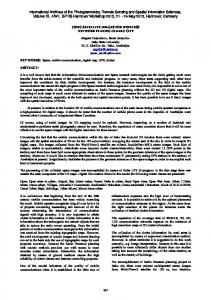
The inventory includes the establishment of a two-hectare plot subdivided into 150 grids each with a dimension of 10x10m. All trees within the plot with DBH greater than 10 cm are geotagged. The height and DBH of these selected trees were also recorded. Figure 2 shows the LAS File (LiDAR Point Cloud) over the subdivided grids and exact location of geotagged trees.

Parameter Canopy Cover Canopy Density

General Statistics

Percentiles

Figure 2: Geotagged trees within the 10x10m grid plots A total of 1,094 trees were surveyed within the two hectares plot. From the 150 grids, 50 random samples were selected to serve as data for calibration for the DBH estimation and also to be comparable to the study of Argamosa (2015) who also used 50 samples. 2.4 LiDAR Data Processing Using Lastools, the corresponding LiDAR data of the plot was normalized to adjust the elevation values before extracting the 27 parameters needed for the estimation. In this situation, the height of the trees with respect to each other would be comparable since they were all treated to be in the same elevation. Figure 3 shows the original and normalized point cloud of the plot.

Bincetiles

LIST OF CANOPY METRICS Variable Canopy Metrics Percentage of points (first returns/all COV first returns) Density of points (number of points/ all DNS returns) Height and Intensity Metrics MIN Minimum MAX Maximum AVG Average STD Standard deviation SKE Skewness KUR Kurtosis QAV Quadratic average Height values/Intensity given the 1st P01 percentile of points Height/ Intensity values given the 5th P05 percentile of points Height values/Intensity given the 10th P10 percentile of points Height values/ Intensity given the 25th P25 percentile of points Height values/ Intensity given the 50th P50 percentile of points Height values/ Intensity given the 75th P75 percentile of points Height values/ Intensity given the 90th P90 percentile of points Height values/ Intensity given the 95th P95 percentile of points Height values/ Intensity given the 99th P99 percentile of points Cumulative Percentage of points given B10 the 10% of height Cumulative Percentage of points given B20 the 20% of height Cumulative Percentage of points given B30 the 30% of height Cumulative Percentage of points given B40 the 40% of height Cumulative Percentage of points given B50 the 50% of height Cumulative Percentage of points given B60 the 60% of height Cumulative Percentage of points given B70 the 70% of height Cumulative Percentage of points given B80 the 80% of height Cumulative Percentage of points given B90 the 90% of height

Table 2: 27 LiDAR Canopy Metrics 2.5 DBH Estimation 2.5.1 Multiple Linear Regression A linear regression python script was created to compute for 27 LiDAR parameter coefficients. The computation of coefficients of the features is done through Least Squares computation. The equation used is shown below:

D = a0 + a1P1 + a2 P2 + ... + an Pn n

D = a0 + ∑ a1P1

(1)

i =1

Figure 3: Raw point cloud of the plot (upper) and the normalized point-cloud (lower) The list of canopy metrics to be derived from LiDAR data are listed in Table 2.

where D= field-measured diameter at breast height (DBH) n= number of parameters


659


P= LiDAR derived parameters a= coeffieients to be determined by the regression The generated estimates for DBH are calculated as the average DBH of trees at a 10x10m grid plot. 2.5.2 Statistical Tests Aside from the coefficient of determination, r-squared, two other statistical tests, namely AIC (Akaike’s Information Criterion) and BIC (Bayesian Information criterion) were used to assess the output of regression analysis. R-squared was used as the threshold of accuracy while AIC and BIC was used to determine which among the parameter combination within the threshold r-squared gives the most accurate estimates.

Skicit learn are freely downloaded python libraries were also added in the script to facilitate the mathematical computation. Numpy was used to make the arrays. Pandas was used to create dataframe. And lastly, the Scikit learn was used to perform the machine learning algorithms that is Linear Regression. Through its metric modules, easier computations of different statistical values are done to determine the robustness of a model. 2.6 Results and Discussion From the field data, the number of trees that fell within each of 50 grids was recorded. The mean DBH per grid were also obtained. The average DBH of each grid ranges from 13cm to 40 cm as shown by Figure 4.

Computing r-squared can be done by squaring the correlation coefficient as shown below:

r=

n(∑ xy) − (∑ x)(∑ y)

[n(∑ x ) − (∑ x)2 ][n(∑ y 2 ) − (∑ y)2 ] 2

(2)

where x= x-coordinate (LiDAR-derived DBH Estimates) y= y-coordinate (Field DBH Estimates) n= number of samples (number of grids)

Figure 4: Average DBH in cm of the 50 sample grids

R-squared shows how many data points fall within the results of the line formed by the regression equation. The higher the value means higher the percentages of points are closer and fitted to the regression line. On the other hand, it is claimed that using AIC and BIC can obtain useful information for model selection together, especially when models needed should be selected by both criteria. The equations used for AIC and BIC are listed below. The

AIC = n + n log 2π + n log(

RSS ) + 2( p + 1) n

The corresponding 27 LiDAR parameters of the 50 grids were then derived using Lastools. Using the automated least squares analysis, with the 27 parameters and measured DBH of each grid as input, an estimated DBH and coefficient of parameters for estimation were obtained. Using all the parameters, the generated DBH estimates have an r-squared of 0.71, AIC of 170.13 and BIC of 221. 75. Other combinations with r-squared greater than 0.71 were also selected. The first run stopped using 24 parameters with an rsquared of 0.71, AIC of 164.26 and BIC of 210.15. Upon plotting the parameters not used in each combination, four (4) significant parameters appeared not to be in used.

(3)

And

BIC = n + n log 2π + n log( where

RSS ) + (log n)( p + 1) n

(4)

n= number of data points Rss= residual sum of squares K= number of parameters

Figure 5: First Run Result Threshold value r2>0.71

AIC and BIC do not give the quality of the accuracy like rsquared. They only the determine the best combination of parameters among the pre-selected combinations on the given threshold of r-squaredAIC and BIC are based on the maximum likelihood estimates of the model parameter. 2.5.3 Python Script Itertools one of the standard library packages available was used to get the best combination of the script. Numpy, Pandas and

The Q. Average, 50th percentile, 10th bincentile and 20th bincentile appeared to be insignificant parameters when obtaining DBH estimates with r2>0.71 as shown in figure 5. The mentioned parameters were then deleted for the next run of least squares. For the next run of least squares, the input matrices are the field DBH of the 50 grids and the 23 remaining parameters of each grid from the first run of least squares. Upon setting the value of r-squared to 0.6, three (3) additional parameters appeared to be not needed for the estimation and they were the minimum,


660


skewness and 40th bincentile. Figure 6 shows the next batch of parameters not being used in the estimation.

Figure 7 shows the field derived DBH against the estimated DBH using the 11-parameter combination. The estimated DBH ranges from 14 to 36 centimeters as opposed to the field data that ranges from 12 cm to 40 centimeters.

Figure 6: Second run of least squares using 23 parameters as input For the third run, 7 parameters were already deleted from the original 27 parameters. The run was continued until no more combination could give an r-squared greater than 0.6. The determination of the best combination underwent 6 (six) run until it reached its threshold. The parameters being removed for each run are summarized in Table 3. ITERATIONS

NO. OF PARAMETERS IN COMBINATIONS WITH R2>0.06

PARAMETERS TO BE REMOVED

First Run 26, 25, 24 Qav, p50, b10, b20 Second Run 23, 22,21, 20 Min, Ske, b40 Third Iteration 20, 19, 18 B60, b80 Fourth Iteration 18, 17, 16 Std, P75, B30 Fifth Run 15, 14, 13 P05, p99, dns Last Run 12, 11 cov Table 3: List of Parameters Removed from LiDAR Combinations

Figure 7: Estimated mean DBH and measured mean DBH per grid

When plotted using XY scatter graph, the plot of the estimated DBH and field DBH gives an RMSE of 3.75 cm at r-squared value of 0.6 as shown in Figure 8.

The final combination using only 11 parameters gave a promising r-squared of 0.604 and has the lowest of AICs and BICs with values 154.04 and 175.08, respectively. There has been a significant changed in AIC and BIC when compared to an r-squared of 0.712, 170.12 AIC and 221.25 BIC when all parameters are used. The canopy-related metrics, cover and density, were both removed from the list of parameters. From the general statistics parameters, only the maximum, average and kurtosis were found to provide positive effect on the estimation. The highest and the lowest of percentiles proved to be not in used, too. On the other hand, the upper limit of the bincentile are highly used in the estimation. The remaining parameters used in the final estimation is shown in Table 4 below: TYPE OF PARAMETER

Canopy-Related General Statistics

Figure 8: Field DBH against Estimated DBH 3. CONCLUSION Estimating DBH of trees has found to be obtainable when parameters directly derived from LiDAR are used. However, not all these parameters contribute to the accuracy of the estimation. Using all this parameter may just cause over parameterization in the process.

PARAMETERS

none Maximum, Average Kurtosis Percentul P01 P10 P90 P95 Percentile B50 B70 B90 Table 4: Parameters Used in the Best DBH Estimation

The removals of unnecessary parameters have been found systematically. Almost same parameters appeared to be not in used when the estimation showed a good result. This study shows that even when using 11 parameters out of the 27 parameters that can be directly derived, a promising estimation can still be generated. Since the distribution of point clouds vary depending on the structure of canopy, different parameter combinations may be good for other forest classification.


661


ACKNOWLEDGEMENT This research work was done under Project 3: Forest Resources Extraction from LiDAR Surveys of Phil-LiDAR 2 Program Nationwide Detailed Resource Assessments of the Philippines. The LiDAR data used are given by Phil-LiDAR 1 Program. Both programs are funded by the Department of Science and Technology- Grant-in-Aid (DOST-GIA) and implemented by the UP Training Center for Applied Geodesy and Photogrammetry. Recognition is also given to Makiling Center for Mountain Ecosystems (MCME) for sharing their field plot data.

REFERENCES [1] Argamosa, R.J.L., Paringit, E.C., Zaragosa, G.P., Bantayan, N.C., Ibañez, C.A.G., Faelga, R.A.G., Posilero, M.A.V., Dimayacyac, N.A., Gonzalvo, K.J., Castillo, M.L., 2015 Estimation of tropical forest tree diameter at breast height from airborne lidar metrics. Asian Conference on Remote Sensing: Philippines [2] Dubayah, R, Drake J.B. (no date). LiDAR Remote Sensing for Forestry Application, Retrieved from http://www2.geog.ucl.ac.uk/~plewis/lidar/jof.pdf on March 2015. [3] Kankare, V., Liang, X., Vastaranta,M., Yu, X., Holopainen,M., and Hyyppä,J., "Diameter distribution estimation with laser scanning based multisource single tree inventory," ISPRS Journal of Photogrammetry and Remote Sensing, Volume 108, Pages 161-171, ISSN 0924-2716 (2015) [4] Kuha, J. “AIC and BIC Comparisons of Assumptions and Performance”, (2014) [5}Isenburg M., (no date). LAStools - efficient tools for LiDAR processing version 111216, Retrieved from http://lastools.org on February 2016. [6] Larget, B. (April 7, 2003). Statistics 33. Retrieved from http://www.stat.wisc.edu/courses/st333-larget/aic.pdf on March 2015 [7]Makiling Center for Mountain Ecosystems (MCME), "Welcome to Mount Makiling", (August 2015) [8] National Oceanic and Atmospheric Administration (NOAA), "What is LiDAR" Silver Spring, MD, USA. (August 2015)

APPENDIX Shown below is the python script to get the best possible combination of LiDAR-derived metrics to estimate DBH using R-squared, AIC and BIC statistics.


662