class-pair-guided multiple kernel learning of ... - ISPRS Archives

The International Archives of the Photogrammetry, Remote Sensing and Spatial Information Sciences, Volume XLII-3/W3, 2017 Frontiers in Spectral imaging and 3D Technologies for Geospatial Solutions, 25–27 October 2017, Jyväskylä, Finland

CLASS-PAIR-GUIDED MULTIPLE KERNEL LEARNING OF INTEGRATING HETEROGENEOUS FEATURES FOR CLASSIFICATION Qingwang Wang 1, Yanfeng Gu 1, *, Tianzhu Liu 1, Huan Liu 1, Xudong Jin 1 1

Dept. of Information Engineering, Harbin Institute of Technology, Harbin, 150001, China - [email protected], [email protected], [email protected], [email protected], [email protected] Commission ΙΙI, WG III/4

KEY WORDS: Class-pair-guided, Classification, Heterogeneous features (HFs), Light detection and ranging (LiDAR), Multispectral images (MSI), Multiple kernel learning (MKL)

ABSTRACT: In recent years, many studies on remote sensing image classification have shown that using multiple features from different data sources can effectively improve the classification accuracy. As a very powerful means of learning, multiple kernel learning (MKL) can conveniently be embedded in a variety of characteristics. The conventional combined kernel learned by MKL can be regarded as the compromise of all basic kernels for all classes in classification. It is the best of the whole, but not optimal for each specific class. For this problem, this paper proposes a class-pair-guided MKL method to integrate the heterogeneous features (HFs) from multispectral image (MSI) and light detection and ranging (LiDAR) data. In particular, the “one-against-one” strategy is adopted, which converts multiclass classification problem to a plurality of two-class classification problem. Then, we select the best kernel from pre-constructed basic kernels set for each class-pair by kernel alignment (KA) in the process of classification. The advantage of the proposed method is that only the best kernel for the classification of any two classes can be retained, which leads to greatly enhanced discriminability. Experiments are conducted on two real data sets, and the experimental results show that the proposed method achieves the best performance in terms of classification accuracies in integrating the HFs for classification when compared with several state-of-the-art algorithms.

1. INTRODUCTION Under the background of the rapid development of aviation and aerospace, the whole trend of technical development in the field of remote sensing is to achieve a better earth observation with higher spatial, spectral and temporal resolution so as to provide more exact and finer information. With the development of sensor hardware technology, it becomes easy realization of the multi-source data acquired from the same observation scene by using different sensors. Hyperspectral image (HSI) can provide a detailed description of the spectral signatures (X, Y, Spectrum) of ground covers. Therefore, it has been widely used in the application of land covers mapping (Melgani and L. Bruzzone, 2004). However, when just using such data, it appears to be inadequate to distinguish the objects composed of similar materials, e.g., between streets and roofs of buildings. Whereas, LiDAR data can provide the height information (X, Y, Z) of the same surveyed area (Filin, 2002), which is complementary to HSI. The fusion of both data sources, with the purpose of completing or enhancing a comprehensive object characterization in spectral, spatial and elevation domains (X, Y, Z, f(X, Y), Spectrum), is important and promising, particularly for heterogeneous environments and steep terrain. The features extracted from HSI and LiDAR data were categorized into three different attributes, i.e., spectral, spatial, and elevation attributes (Gu and Wang, 2015). Once considered together these complementarity can be helpful for characterizing land use.

Different studies have already proven the potential of integrating HSI and LiDAR data for various areas of research. For data analysis and classification procedures, the elevation information serves as an additional dimension to enhance information content and classification results. Many techniques have been developed for fusion of these heterogeneous features in a classification task. Summing these fusion strategies up, they can be broadly divided into five categories: based on the feature stack structure (Puttonen et al., 2011), hierarchical scheme (Paris and Bruzzone, 2015), sparse representation (Zhang and Prasad, 2016), manifold learning or graphs (Gu and Wang, 2017), and multiple kernel learning (MKL) (Gu and Wang, 2015). Koetz et al. (2007) classified fuel composition from fused LiDAR and hyperspectral bands using support vector machines (SVMs) and showed that the classification accuracies after fusion were higher than those based on either sensor alone. Pedergnana et al. (2012) proposed a technique performing a classification of the features extracted with extended attribute profiles (EAPs) computed both on optical and LiDAR images for an urban area of the city of Trento, leading to a fusion of the spectral, spatial and elevation information in a stacked architecture. Strategies based on the feature stack structure were verified that the fusion strategies do not always perform better than only using a single feature source (Mura et al., 2011). Fusion strategies based on hierarchical scheme for HSI and LiDAR data firstly process one data source in a classifier and then integrate its output with another data source to obtain the

* Corresponding author

This contribution has been peer-reviewed. https://doi.org/10.5194/isprs-archives-XLII-3-W3-195-2017 | © Authors 2017. CC BY 4.0 License.

195

The International Archives of the Photogrammetry, Remote Sensing and Spatial Information Sciences, Volume XLII-3/W3, 2017 Frontiers in Spectral imaging and 3D Technologies for Geospatial Solutions, 25–27 October 2017, Jyväskylä, Finland

final results. A 3-D model-based approach was proposed to the estimation of the tree top height based on the fusion between low-density LiDAR data and high-resolution optical images (Paris and Bruzzone, 2015). In their proposed approach, the integration of the two remote sensing data sources was first exploited to accurately detect and delineate the single tree crowns. Then, the LiDAR vertical measures were associated to those crowns hit by at least one LiDAR point and used together with the radius of the crown and the tree apex location derived from the optical image for reconstructing the tree top height by a properly defined parametric model. Fusion strategies based on sparse representation and multi-task learning fuse the heterogeneous features by dictionary construction and sparse coefficient solution (Jia et al., 2016). Fusion strategies based on manifold learning fuse the heterogeneous features by mining the manifold structure of these features. A generalized graph-based fusion method was proposed to couple dimension reduction and feature fusion of the original HSI and MPs (built on both HSI and LiDAR data) (Liao et al., 2015). In their proposed method, the edges of the fusion graph were weighted by the distance between the stacked feature points. A novel discriminative graph-based fusion (DGF) method was proposed for urban area classification to fuse heterogeneous features from HSI and LiDAR data (Gu and Wang, 2017). The edges of the graphs are measured by kernel. Furthermore, the multi-scale DGF (MSDGF) was introduced to utilize the capability of similarity measure of different scales of kernel and avoid finding the optimal scale simultaneously. Fusion strategies based on MKL are an effective kernel-based framework for integrating multisource data (Camps-Valls et al., 2008). Camps-Valls et al. (2008) first proposed a kernel-based fusion framework to integrate heterogeneous information from multi-temporal and multi-source remote sensing data for classification and change detection. Four ways to form composite kernel were given in their work, including stack, direct summation, weighted summation, and cross-information. The results of their study indicate that direct summation composite kernel yielded better results and achieved a higher efficiency in the particular application domain of urban monitoring, outperforming the traditional stacked-vector approach in real-scenario cases. A novel MKL model of integrating MSI and LiDAR data by fusing those heterogeneous features for urban arear classification has been proposed (Gu and Wang, 2015). In their work, First, Gaussian kernels with different bandwidths were used to measure the similarity of samples on each feature at different scales. Then, these multiscale kernels with different features were integrated using a linear combination. In the combination, the weights of the kernels with different features were determined by finding a projection based on the maximum variance. Finally, the optimization of the conventional support vector machine with this combined kernel was performed to construct a more effective classifier. MKL provides a flexible framework for us to fuse different sources of information in a very natural way. The complementary and relevant information contained in HSI and LiDAR data can be fused and utilized by taking into account the basic kernels construction and its optimizing configuration in MKL. The existing MKL methods mainly include two steps. Basic kernels are constructed in first step. Then the basic kernels are combined in a linear or nonlinear way. The combined kernel learned by MKL can be regarded as the compromise of all basic kernels for all classes in classification. It is the best of the whole, but not optimal for each specific class. For this problem, in this paper, the “one-against-one” strategy is

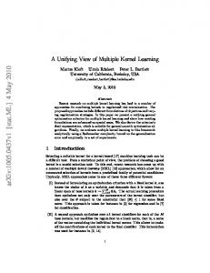
Figure 1. Multiscale kernel matrices for training samples of Bayview Park data set. adopted, which converts multiclass classification problem to a plurality of two-class classification problem. Then, we select the best kernel from pre-constructed basic kernels set for each class-pair by kernel alignment (KA) in the process of classification. The remainder of this paper is organized as follows. The proposed method is introduced in detail in Section 2. Section 3 describes the data set and the experimental setup, and presents the experimental results on two real data sets and compares the proposed method with other fusion methods. Finally, conclusions are drawn in Section 4. 2. PROPOSED METHOD The literature (Gönen and Alpaydin, 2011) points out that combining kernels in a nonlinear or data-dependent way seems more promising than linear combination when fusing simple linear kernels, whereas linear methods are more reasonable when combining complex Gaussian kernels. In this paper, we consider the latter choice and employ the popular Gaussian kernel with different bandwidths. Here, Gaussian kernel is given as follows:

K (xi , x j )  exp(

xi  x j 2 2

2

),  



(1)

where  is a radius parameter called bandwidth. The bandwidth of Gaussian kernel controls smoothness of kernel measure. With large value of bandwidth, the kernelized distance measure is smooth. As a result, kernel value is insensitive to small variation of similarities. And with small value of bandwidth, it is opposite that the kernel is sensitive to variation of similarities, but may result in a highly diagonal kernel matrix which loses generalization capability. Therefore, bandwidth can be regarded as a scale under which kernel compares samples, and this scale controls the kernel resolution which means the discriminative ability of kernel. We take the Bayview Park data set for an instance to demonstrate the multiscale property of kernel similarity measure. Scales of basic kernels are uniformly selected in the interval of [0.2, 2] with a step size of o.2, and the multiscale kernel matrices are shown in Figure 1. According to the visualization of kernel matrices in Figure 1, the similarity measure presents good multiscale property. It is well known that the kernel method transforms the linearly inseparable problem in the original data space into a linear separable problems in reproducing kernel Hilbert space by using a nonlinear mapping function. If a mapping function

This contribution has been peer-reviewed. https://doi.org/10.5194/isprs-archives-XLII-3-W3-195-2017 | © Authors 2017. CC BY 4.0 License.

196

2 1.5 1 0.5 0 0

10 20 Different class pairs

30

 with highest KA score

 with highest KA score

The International Archives of the Photogrammetry, Remote Sensing and Spatial Information Sciences, Volume XLII-3/W3, 2017 Frontiers in Spectral imaging and 3D Technologies for Geospatial Solutions, 25–27 October 2017, Jyväskylä, Finland

2

Taking the reserved kernel K c2 into support vector machine

1.5

(SVM) classifier can form our optimization problem (a convex quadratic programming problem) for each two-class classification problems as follows:

1 0.5 0 0

20 40 Different class pairs

60

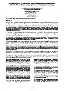
(a) Bayview park (b) Recology Figure 2.  with highest KA scores of different class pairs. exists between samples and the corresponding labels, the mapped spaces will be constituted by class labels. Apparently, the samples are linear separable in this resulting space because of distinct labels for different classes. The corresponding kernel is called ideal kernel that can be computed by inner product of labels for binary classifier. The Gram matrix of ideal kernel is notated as K I , and the values of K I are computed by  0, yi  y j K I ( xi , x j )    1, yi  y j

(2)

KA is a measure of the similarity between two kernel matrices. And the alignment score between two kernel matrixes K 1 and K 2 is defined as follows:

K1 , K 2 K1 , K1

F

F

K2,K2

(3)

=i 1  j 1 K1  xi , x j  K2  xi , x j  . N

F

(5) i , j  1, 2,

,N

where  i and  j are Lagrange multipliers, and if  i is nonzero, the corresponding x i is called a support vector, which determines the decision hyperplane. After solving the above optimization problem, we can get the classification decision function. For a test sample x, the label is determined by following classification decision function. (6)

where  i is a support vector, and n is number of support vectors. The final class label of the sample x is determined by counting the majority of classification results of the separating two-class classification problems. The procedure of the proposed method

F

where  ，  F is the Frobenius norm between two matrices and defined as K1 , K 2

N  i yi  0 s.t.  i 1  ,   0,C ,  i j

n  f (x)  sgn  i yi Kc2  xi , x   b   i 1 

where yi is the class label of sample x i .

s  K1 , K 2  

N 1 N N   max Q  i , j    i   i j yi y j K c2  xi , x j   2 i 1 j 1   i 1

N

We utilize “one-against-one” strategy to solve multiclass classification problem. When classifying C classes, we divide the training samples of each two classes into a group, and we can get a total of  C  C  1  / 2 groups. We compute the KA scores of each basic kernel constructed by using each two classes ( c2 : class i and class j) and ideal kernel, and reserve the basic kernel with highest score for the class pair of class i and class j.

i) Initialize the range of kernel scale values [  min ,  max ]. ii) Sample M scales within the range above, i.e.,  min  1   2  M   max . iii) Select the optimal kernel scale for each class pair by utilizing a principle of the highest KA scores. iv) Under the “one-against-one” classification strategy, take the optimal kernels determined in iii) into (5) for each two-class classification problems. v) Determine the class label of test samples by counting the majority of classification results of the separating two-class classification problems. 3. RESULTS AND VALIDATION

 x x c i c j K c2 xc2 i , xc2 j  exp   2 2 2  2 c 





2

   

(4)

For example, the range of bandwidth of Gaussian kernel was set to [0.05, 2], and uniform sampling that selects scales from the interval with a fixed step size of 0.05 was used to select 40 scales within the given range. The bandwidths  with highest KA score of different class pairs are shown in Figure 2. Bayview park data set has 7 classes. Thus there is  7   7-1 / 2  21 class pairs in this data set. As the same principle, Recology data set has 55 class pairs. We can find that the different class pairs correspond to different bandwidths  with highest KA score.

In order to verify the effectiveness of the proposed method, two data sets are used, and two experiments are designed. In this section, we test the performance of the proposed method and comparison methods for joint classification of MSI and LiDAR data. 3.1 Data description The two data sets are from two subregions of a whole scene around downtown area of San Francisco, USA. One is located at a factory named “Recology” and the other is located at a park named “Bayview Park”. The data come from 2012 IEEE GRSS Data Fusion Contest and contain multispectral images (8 bands in the wavelength range of 400 to 1040 nm) and the corresponding LiDAR data. The multispectral images were

This contribution has been peer-reviewed. https://doi.org/10.5194/isprs-archives-XLII-3-W3-195-2017 | © Authors 2017. CC BY 4.0 License.

197

The International Archives of the Photogrammetry, Remote Sensing and Spatial Information Sciences, Volume XLII-3/W3, 2017 Frontiers in Spectral imaging and 3D Technologies for Geospatial Solutions, 25–27 October 2017, Jyväskylä, Finland

95

OA(%)

建筑物3 道路 树木 裸地 海水 背景

(c)

Figure 3. Bayview Park data set. (a) RGB composite image of bands. (c) Ground truth map. 建筑物1 建筑物2 建筑物3

85 80

Kappa coefficient

建筑物2

(a)

0.9

90

建筑物1

0.85 0.8 0.75

SK SK 0.7 SimpleMKL SimpleMKL 75 MeanMKL MeanMKL 0.65 RMKL RMKL C2MKL C2MKL 70 0.6 10 15 20 30 40 50 100 10 15 20 30 40 50 100 Number of training samples per class Number of training samples per class

(a) (b) Figure 5. OA (a) and Kappa coefficient (b) of different methods on Bayview Park data set.

建筑物4 建筑物5

90

建筑物6 树木

80

裸地 草地

(a)

(b)

背景

OA (%)

停车场

75 70

0.75 0.7 0.65

SK SK SimpleMKL SimpleMKL 0.6 MeanMKL MeanMKL 60 0.55 RMKL RMKL C2MKL C2MKL 55 0.5 10 15 20 30 40 50 100 10 15 20 30 40 50 100 Number of training samples per class Number of training samples per class 65

Figure 4. Recology data set. (a) RGB composite image of bands. (b) Ground truth map.

0.8 Kappa coefficient

85

建筑物7

(a) (b) Figure 6. OA (a) and Kappa coefficient (b) of different methods on Recology data set.

acquired by WorldView2 on 9th Oct, 2011 and the LiDAR data were acquired in June 2010. The two data sets have a spatial resolution of 1.8m. Figures 3 and 4 show the false RGB composition and information of the labelled classes for the two selected study areas, respectively. We identified the land cover classes in the two data sets by visual inspection with the help of Google Earth. The land cover classes in the Bayview Park data set are “Building1”, “Building2”, “Building3”, “Road”, “Trees”, “Soil” and “Seawater”. The reference land cover classes of Recology data set are “Building1”, “Building2”, “Building3”, “Building4”, “Building5”, “Building6”, “Building7”, “Trees”, “Parking lot”, “Soil” and “Grass”. The two data sets are both the combination of multispectral images and LiDAR data. It is noteworthy that the two data sets are classified as different classes according to heights and materials of land-covers. The main characteristics of the data sets are summarized in Table 1. 3.2 Experimental setup To validate the proposed method (C2MKL for short), we compare it with several state-of-the-art methods. They are single kernel SVM (SK for short), RKML (Gu et al., 2012), Mean MKL (Gönen and Alpaydin, 2011), Simple MKL (Rakotomamonjy et al., 2008). For all the classifiers, the range

of bandwidth of Gaussian kernel was set to [0.05, 2], and uniform sampling that selects scales from the interval with a fixed step size of 0.05 was used to select 40 scales within the given range. For the model parameters of SVM which were used in all classifiers in our experiments, the penalization parameter is selected by Cross-Validation (CV) in the range of [101, ,107 ] and the slack variable   107 also is selected by CV. Two experiments are designed to verify the fusion ability of the proposed method. The first experiment is a low-level fusion for spectral image and LiDAR data. In particular, joint classification with spectrum (8 spectral bands) and normalized digital surface model (nDSM) extracted from LiDAR data are considered. The second experiment is an extended fusion for spectral image and LiDAR data. The spectrum, spatial features and nDSM are fused in this experiment for classification. The spatial features are the morphological profiles (MPs), and MPs are computed on two windows of size 3x3 and 5x5 pixels. The dimension of the morphological features is 8 (with 2 opening and 2 closing for the first principal component of spectral bands and the same number for the LiDAR data). The heterogeneous features from MSI and LiDAR data were stacked into a feature vector. Then, the extended feature vector is input into Gaussian kernel with different bandwidths to generate the basic kernels. In each experiment, the labelled training samples were randomly selected. The number of training samples for each class was set to 10, 15, 20, 30, 40, 50 and 100. The rest of the samples were used as test samples. Each experiment was conducted with 10 trials to avoid biased conclusions and the average results and variance were reported. Overall accuracy (OA), Kappa statistic and classification maps were considered to evaluate all classifiers.

This contribution has been peer-reviewed. https://doi.org/10.5194/isprs-archives-XLII-3-W3-195-2017 | © Authors 2017. CC BY 4.0 License.

198

The International Archives of the Photogrammetry, Remote Sensing and Spatial Information Sciences, Volume XLII-3/W3, 2017 Frontiers in Spectral imaging and 3D Technologies for Geospatial Solutions, 25–27 October 2017, Jyväskylä, Finland

100

1

95

OA (%)

Kappa coefficient

0.9

90

0.8

85

SK 80 SimpleMKL MeanMKL 75 RMKL C2MKL 70 10 15 20 30 40 50 100 Number of training samples per class

SK SimpleMKL MeanMKL RMKL C2MKL 0.6 10 15 20 30 40 50 100 Number of training samples per class SK 0.7

SK SK SK

(a) SK

Simple SK MKL

Simple Simple MKL MKL Simple MKL

(b) Simple MKL Mean MKL SK Simple MKL

Mean Mean MKL MKL Mean MKL

(c) Mean MKL Simple MKL Mean MKL

Mean MKL

(a) (b) Figure 7. OA (a) and Kappa coefficient (b) of different methods on Bayview Park data set. 100

1

OA (%)

90 85 80 75 70

SK SimpleMKL MeanMKL RMKL C2MKL

65 10 15 20 30 40 50 100 Number of training samples per class

Kappa coefficient

95 0.9 RMKL RMKL RMKL

0.8

0.7

RMKL

SK SimpleMKL MeanMKL RMKL C2MKL

C2MKL RMKL

(c) RMKL

C2MKL C2MKL C2MKL

真实地物分布图 RMKL C2MKL

(d) C2MKL

真实地物分布图 真实地物分布图 真实地物分布图

C2MKL 真实地物分布图

(e) Ground truth map

Figure 9. Classification maps of different methods on Bayview Park data set.

0.6 10 15 20 30 40 50 100 Number of training samples per class

(a) (b) Figure 8. OA (a) and Kappa coefficient (b) of different methods on Recology data set. 3.3 Experimental results 3.3.1 Experiment 1: joint classification with spectrum and nDSM : Joint classification with spectrum and nDSM which is the simplest features setting to joint use of spectral image and LiDAR data was carried out. Numerical classification results of our proposed method (C2MKL) and four contrast methods (SK, SimpleMKL, Mean MKL and RMKL) are shown in Figures 5 and 6. From the experimental results, we can see that our proposed method achieves the highest classification accuracy under different training samples. This proves that our proposed method can effectively fuse the heterogeneous features from MSI and LiDAR data to improve classification performance. 3.3.2 Experiment 2: Joint classification with spectrum, MPs and nDSM: Joint classification with the spectrum (spectral attributes), MPs (spatial attributes) and nDSM (elevation attributes) was carried out and the numerical results of classification for two data sets are shown in Figures 7 and 8. Our proposed method achieves the highest classification accuracy once again. Complementary information between spectral, spatial, and elevation features can be further explored for classification task by our proposed method. Compared with experiment 1, experiment 2 achieves a higher classification accuracy. This shows that adding spatial features can provide useful information to improve classification performance. This also shows that there are complementary information between the features of different attributes. Combining features of different attributes can improve the classification performance.

SK (a)SK SK

Mean MKL

Mean MKL (c) Mean MKL

Simple MKL MKL Simple (b) Simple MKL

RMKL

RMKL (c) RMKL

C2MKL 真实地物分布图 (d) C2MKL (e) Ground truth map Figure 10. Classification maps of different methods on Recology data set.

classification maps, we can visually see that our proposed C2MKL gets the best performance as compared to the other classifiers. Furthermore, we observe that the misclassification generally occurs at the edges of each class. The black rectangles in the classification maps are the places with significant improvement of C2MKL compared to other classifiers.

We show the classification maps in Figure 9 for Bayview Park data set and Figure 10 for Recology data set. From the

This contribution has been peer-reviewed. https://doi.org/10.5194/isprs-archives-XLII-3-W3-195-2017 | © Authors 2017. CC BY 4.0 License.

199

真实地物分布图

The International Archives of the Photogrammetry, Remote Sensing and Spatial Information Sciences, Volume XLII-3/W3, 2017 Frontiers in Spectral imaging and 3D Technologies for Geospatial Solutions, 25–27 October 2017, Jyväskylä, Finland

4. CONSLUSION In this paper, we proposes a class-pair-guided MKL method to integrate the heterogeneous features from MSI and LiDAR data. The proposed method solves the problem that the combined kernel learned by conventional MKL methods is a compromise of all basic kernels for all classes in classification, and is the best of the whole, but not optimal for each specific class. For joint classification of MSI and LiDAR data, two different fusion experiments are carried out. The experimental results show that our method can improve the classification accuracy and validate the helpfulness of our method for classification task. The two experiments verify that there are complementary information between the features of different attributes. Combining features of different attributes can improve the classification performance.

ACKNOWLEDGEMENTS This work was supported by the National Science Fund for Excellent Young Scholars under the Grant 61522107 and the Natural Science Foundation of China under the Grant 61371180. This work was also supported by China Aerospace Science and Technology Corporation - Harbin Institute of Technology Joint Center for Technology Innovation Fund (No.CASC-HIT151C03). We would like to thank the Image Analysis and Data Fusion Technical Committee (IADFTC) of the IEEE Geoscience and Remote Sensing Society (GRSS) for providing the experimental data sets.

Koetz, B., Sun, G., Morsdorf, F., Ranson, K. J., Kneubuhler, M., Ltten, K., and Allgower, B., 2007. Fusion of imaging spectrometer and LIDAR data over combined radiative transfer models for forest canopy characterization. Remote Sens. Environ., 106(4), pp. 449-459. Pedergnana, M., Marpu, P. R., Mura, M. D., Benediktsson, J. A., and Bruzzone, L., 2012. Classification of Remote Sensing Optical and LiDAR data Using Extended Attribute Profiles. IEEE Journal of Selected Topics in Signal Processing, 6(7), pp. 856-865. Mura, M. D., Villa, A., Benediktsson, J. A., Chanussot, J., and Bruzzone, L., 2011. Classification of hyperspectral images by using extended morphological attribute profiles and independent component analysis. IEEE Geosci. Remote Sens. Lett., 8(3), pp. 541-545. Sen, J., Jie, H., Yao, X., Linlin, S., Xiuping, J., and Qingquan, L., 2016. Gabor Cube Selection Based Multitask Joint Sparse Representation for Hyperspectral Image Classification. IEEE Trans. Geosci. Remote Sens., 54(6), pp. 3174-3187. Wenzhi, L., Pizurica, A., Bellens, R., Gautama, S., and Philips, W., 2015. Generalized Graph-Based Fusion of Hyperspectral and LiDAR Data Using Morphological Features. IEEE Trans. Geosci. Remote Sens. Lett., 12(3), pp. 552-556. Camps-Valls, G., Gomez-Chova, L., Munoz-Mari, J., RojoAlvarez, J. L., and Martinez-Ramon, M., 2008. Kernel-Based Framework for Multitemporal and Multisource Remote Sensing Data Classification and Change Detection. IEEE Trans. Geosci. Remote Sens., 46(6), pp. 1822-1835.

REFERENCES Melgani, F., and Bruzzone, L., 2004. Classification of hyperspectral remote sensing images with support vector machines. IEEE Trans. Geosci. Remote Sens., 42(8), pp. 17781790. Filin, S., 2002. Surface clustering from airborne laser scanning data. In Proc. ISPRS Commission III Symp. Photogramm. Comput. Vis., 34(3), pp. 119-124.

Gönen, M., and Alpaydin, E., 2011. Multiple kernel learning algorithms. J. Mach. Learn. Res., 12, pp. 2211-2268. Yanfeng, G., Chen, W., Di, Y., Yuhang, Z., Shizhe, W., and Ye, Z., 2012. Representative Multiple-kernel Learning for Classification of Hyperspectral Imagery. IEEE Trans. Geosci. Remote Sens., 50(7), pp. 2852-2865. Rakotomamonjy, A., Bach, F. R., Canu, S. and Grandvalet, Y., 2008. SimpleMKL. J. Mach. Learn. Res., 9(3), pp. 2491-2521.

Yanfeng, G., Qingwang, W., Xiuping, J., and Benediktsson, J. A., 2015. A novel MKL model of integrating LiDAR data and MSI for urban area classification. IEEE Trans. Geosci. Remote Sens., 53(10), pp. 5312-5326. Puttonen, E., Jaakkola, A., Litkey, P., and Hyyppä, J., 2011. Tree classification with fused mobile laser scanning and hyperspectral data. Sensors, 11, pp. 5158-5182. Paris, C., and Bruzzone, L., 2015. A three-dimensional modelbased approach to the estimation of the tree top height by fusing low-density LiDAR data and very high resolution optical images. IEEE Trans. Geosci. Remote Sens., 53(1), pp. 467-480. Yuhang, Z., and Prasad, S., 2016. Multisource geospatial data fusion via local joint sparse representation. IEEE Trans. Geosci. Remote Sens., 54(6), pp. 3265-3276. Yanfeng, G. and Qingwang, W., 2017. Discriminative GraphBased Fusion of HSI and LiDAR Data for Urban Area Classification. IEEE Geosci. Remote Sens. Lett., 14(6), pp. 906910.

This contribution has been peer-reviewed. https://doi.org/10.5194/isprs-archives-XLII-3-W3-195-2017 | © Authors 2017. CC BY 4.0 License.

200