PHYSICAL REVIEW E 81, 031916 共2010兲
Estimating input parameters from intracellular recordings in the Feller neuronal model Enrico Bibbona* Department of Mathematics G. Peano, University of Torino, Via Carlo Alberto 10, 10123 Torino, Italy
Petr Lansky† Institute of Physiology, Academy of Sciences of the Czech Republic, Videnska 1083, 142 20 Prague 4, Czech Republic
Roberta Sirovich‡ Department of Mathematics G. Peano, University of Torino, Via Carlo Alberto 10, 10123 Torino, Italy 共Received 10 November 2009; published 25 March 2010兲 We study the estimation of the input parameters in a Feller neuronal model from a trajectory of the membrane potential sampled at discrete times. These input parameters are identified with the drift and the infinitesimal variance of the underlying stochastic diffusion process with multiplicative noise. The state space of the process is restricted from below by an inaccessible boundary. Further, the model is characterized by the presence of an absorbing threshold, the first hitting of which determines the length of each trajectory and which constrains the state space from above. We compare, both in the presence and in the absence of the absorbing threshold, the efficiency of different known estimators. In addition, we propose an estimator for the drift term, which is proved to be more efficient than the others, at least in the explored range of the parameters. The presence of the threshold makes the estimates of the drift term biased, and two methods to correct it are proposed. DOI: 10.1103/PhysRevE.81.031916
PACS number共s兲: 87.10.⫺e, 87.19.L⫺, 02.50.⫺r, 05.40.⫺a
I. INTRODUCTION
Stochastic leaky integrate-and-fire 共LIF兲 models are among the most popular mathematical descriptors for the neuronal activity 关1–4兴. These are simple models that reproduce with a reasonable degree of approximation the response of a neuron or complex neuronal models 关5兴. They appear in many variants; in all of them the membrane potential is described as a stochastic process, whereas the spike generation is due to the crossing of a threshold level by the process. The most common stochastic LIF model is based on the OrnsteinUhlenbeck process 关6–9兴. In that model the synaptic transmission is state independent and the membrane potential is not limited from below 共nor from above, apart that if the threshold is reached a spike is generated and the process is reset兲. As a consequence it may happen that the membrane potential reaches unrealistic low values. In order to prevent such events, modifications that better characterize the process of synaptic transmission by inclusion of reversal potentials were proposed and explored 关10,11兴. Here we consider one of the variants of the LIF model with inhibitory reversal potential in which the membrane potential is described by the so-called Feller process. This model with multiplicative noise includes state-dependent inputs and ensures that the membrane potential fluctuations are limited by an inaccessible lower boundary as the effect of the inhibitory postsynaptic potential decreases if the membrane potential gets closer to it. The quality of a model, however, should be judged on the basis of a quantitative comparison with real data. Starting
*
[email protected] †
[email protected] [email protected]
‡
1539-3755/2010/81共3兲/031916共13兲
from 关12–15兴, for many years only few papers were dedicated to this problem 关16–20兴, but recently attention to this topic began to grow. Attempts to establish a benchmark test that permits a comparison between the predictive capability of different single neuron models over a broad range of firing rates and firing patterns were suggested in 关21兴 and two competitions, the neural prediction challenge 关22兴 and the quantitative single neuron model competition 关23兴, took place. This effort aims at prediction of the output from the knowledge of the input. From a statistical point of view, the first step in the direction of comparing output data with output produced by the models is an efficient estimation of the parameters. The input signal is the most relevant parameter of the model 关24,25兴. Experimental data are essentially of two kinds—extracellular and intracellular recordings. In the former case just the sequence of firing times is registered, and parameter 共signal兲 estimation for data of that kind was studied, for example, in 关26–29兴 and a review can be found in 关30兴. In the latter case the trajectory of the membrane potential is sampled at discrete times. Statistical methods for the estimation of the parameters from discretized trajectories are available for a large class of processes 关31,32兴. The application to the stochastic neuronal models is not obvious due to the presence of the absorbing threshold which has been shown to bring a bias in the maximum likelihood estimator of the drift parameter 关33兴.Only few references 关34–36兴 provide statistical methods dedicated to parameter estimation for randomly stopped processes, but they are restricted to very special cases. In the present paper we focus on the Feller model and estimation of its input parameters from a sampled trajectory. Some studies were already performed outside the neuronal context but only in the absence of the threshold 关37–39兴. Thus, we have several different estimators whose performances should be compared in a parameter range expected
031916-1
©2010 The American Physical Society
PHYSICAL REVIEW E 81, 031916 共2010兲
BIBBONA, LANSKY, AND SIROVICH
for neuronal data and in the presence of the threshold. The Feller process was first introduced in 关40兴 as an example of a singular diffusion process and it has many applications apart from neuronal modeling. Well known is a model of short term interest rates as proposed in 关41兴 from where the mathematical finance community adapted its name to Cox Ingersoll Ross process. More recently it has been used to model nitrous oxide emission from soil 关42兴 or, in the framework of survival analysis theory, to model the individual hazard rate 关43兴. In Sec. II we review the relevant properties of the Feller process. Some methods for the estimation of the input parameters are reviewed and a different one is introduced in Sec. III. In Sec. IV a complete comparison of the different estimators both in the absence and in the presence of the absorbing threshold is performed. Finally methods to improve the estimates in the presence of the threshold are proposed. II. MODEL
One of the most common models for the neuronal depolarization is the Ornstein-Uhlenbeck diffusion process Ut which can be given in the form of the following stochastic differential equation:
冉
冊
Ut − u0 dUt = − + U dt + UdWt, U
U0 = u0 ,
共1兲
where u0 is the resetting and resting potential, U ⬎ 0 is the membrane time constant, U is the drift parameter, U ⬎ 0 is the diffusion coefficient, and Wt is a standard Brownian motion 共Wiener process兲. The physiology of the cell does not allow the membrane potential to reach too low values and a better model should include a lower bound of the depolarization. In 关11兴 the following model was proposed. The evolution of the membrane potential is described by the process Y t in the form of the following stochastic differential equation:
冉
dY t = −
冊
Y t − y0 + Y dt + 冑Y t − VIY dWt,
intracellular recordings are available, true data are in some cases much better fitted by model 共2兲 with respect to a simple Ornstein-Uhlenbeck. A translated form Xt = Y t − VIY of the process allows us to get rid of one of the parameters y 0 and VIY . If parameters are mapped as follows,
Y = −
VIY = − x0 + y 0 , the Feller process Xt is the solution of the stochastic differential equation,
冉
dXt = −
冊
Xt + dt + 冑XtdWt,
E共Xt兩X0, 兲 = X0e−t/ + 共1 − e−t/兲.
共3兲
共4兲
Conditional variance and covariance are Var共Xt兩X0, , 2兲 = 2v共Xt兩X0, 兲
= 2 共1 − e−t/兲关共1 − e−t/兲 + 2X0e−t/兴 2 共5兲 and Cov共Xt,Xs兩X0, , 2兲 = e−共t−s兲/ Var共Xs兩X0, , 2兲
共6兲
for s ⬍ t. The process is time homogeneous and the transition density function f共xt , t 兩 x0兲 is 关40,41兴 f共x,t兩x0兲 = ce−r−s
is the resetting and resting potential, ⬎ 0 is where the membrane time constant, Y is the drift parameter, and ⬎ 0 is the diffusion coefficient. Comparing Eqs. 共1兲 and 共2兲 we can see their identical behavior with vanishing noise. Under the presence of the noise its amplitude in Eq. 共2兲 changes with the actual value of the depolarization, whereas in Eq. 共1兲 it remains constant. The main difference between the models is caused by the new parameter VIY which is the minimum value allowed for the membrane potential and it is called inhibitory reversal potential. If the parameters satisfy condition 2Y + 2VIY − 2y 0 ⱖ 2 the process starting above VIY never reaches that value 关40兴. In 关44兴 the qualitative behavior of the Ornstein-Uhlenbeck and Feller models was compared showing that if parameters are suitably chosen, the two models provide rather similar spike trains 共i.e., the sequence of firing times兲. In 关19兴 it was shown that as long as
X0 = x0 ,
where x0 ⬎ 0 is the resetting point and the inhibitory reversal potential is shifted to the zero level. For 2 ⱖ 2 the zero value is an inaccessible barrier 共an entrance boundary according to Feller’s classification 关40兴兲; this is a reasonable assumption in the context of neuronal modeling 关27兴 and it holds true in all parametric range explored in this paper. The conditional expectation of process 共3兲 is
Y 0 = y0 , 共2兲
x0 ,
冉冊 s r
q/2
Iq共2冑rs兲,
共7兲
where
y 0 ⬎ VIY
c=
2 , 2共1 − e−t/兲 r = cx0e−t/,
q=
2 − 1, 2
s = cx,
and Iq共 · 兲 is the modified Bessel function 关45兴. Generation of the action potentials is not a part of membrane potential model 共3兲. To make the cell fire, a firing threshold is imposed at level S ⬎ x0. The first time the process reaches the boundary level, an action potential is elicited and the membrane potential is instantaneously reset to x0. Then the evolution restarts anew according to the same law. The times between each consecutive couple of spikes 共called interspike intervals兲 follow the distribution of the random variable T = inf兵t ⱖ 0 兩 Xt ⱖ S其 that is often referred to as the first-passage time across the barrier. The most important
031916-2
ESTIMATING INPUT PARAMETERS FROM …
PHYSICAL REVIEW E 81, 031916 共2010兲
characteristic of the random variable T is its mean 关44兴 ⬁
E共T兲 =
S − X0 +兺 j=1
共S j+1 − X0j+1兲
共8兲
j
共j + 1兲 兿 共 + k2/2兲
TABLE I. Summary of estimation methods and properties in the absence of the threshold. An asterisk means that the estimator would be unbiased if the true value of was known. C means consistency, AN means asymptotic normality, O is optimality in the sense of 关48兴, and AE denotes asymptotic efficiency. Method
k=0
Least squares
as it is inversely proportional to the neuronal firing rate. We will use it to check the precision of our numerical experiments. The properties of the model firing are often related to the position of asymptotic depolarization 共3兲 with respect to S and are called subthreshold or suprathreshold regimens. Let us remark that the presence of the threshold is a constraint on the process and its characteristics, such as the accessibility of the states, the transition density, and the moments, are altered. Following the construction of the model as diffusion approximation of a model with discontinuous trajectories, the parameters could be divided into two classes: parameters characterizing the input and intrinsic parameters characterizing the neuron irrespectively of the incoming signal. However, for model 共3兲, such a classification of the parameters is not so straightforward as for the Ornstein-Uhlenbeck model. Indeed, S and x0 remain independent on the input, but the membrane time constant is input dependent 共for details see 关11兴兲. Nevertheless, we assume that these three parameters are known and we focus on the estimation of the remaining two parameters, and , which characterize the input. III. ESTIMATORS FOR THE INPUT PARAMETERS
All the estimation methods presented here are designed to n of prowork on a sample made of a single trajectory 兵Xi其i=1 cess 共3兲 recorded at discrete times ti = ih with constant sampling interval h. Some of them lead to explicit estimators and others to quasilikelihood functions to be minimized or maximized numerically. The presence of the threshold is not accounted for in the estimation methods, however in numerical experiments we thoroughly investigate its effect. All the estimation methods and their main properties are summarized in Table I.
Conditional least squares Gauss-Markov Bibby-Sørensen Optimal estimating function Maximum likelihood
Estimator
Properties
ˆ LS 2 ˆ LS ˆ CLS 2 ˆ CLS ˆ GM ˆ BS 2 ˆ BS ˆ OEF ˆ ML 2 ˆ ML
Unbiased ⴱ Unbiased ⴱ Unknown C, AN C, AN C, AN, O C, AN, AE C, AN, AE
n
2 ˆ LS =
ˆ LS兲兴2v共Xi兩X0, ˆ LS兲 关Xi − E共Xi兩X0, 兺 i=1 n
共10兲
,
ˆ LS兲 v 共Xi兩X0, 兺 i=1 2
ˆ LS兲 and v共Xi 兩 X0 , ˆ LS兲 are where the functions E共Xi 兩 X0 , given by Eqs. 共4兲 and 共5兲. For the estimation of , the residuals ei = Xi − E共Xi 兩 X0 , 兲 are neither independent nor identically distributed. Thus, the asymptotic normality of the estimates is not obvious. However, as one can directly verify ˆ LS is unbiased. Its variance is using Eq. 共4兲, the estimator given by formula 共A1兲. Estimator 共10兲 would be unbiased if ˆ LS. the true value of the parameter was used instead of B. Conditional least-squares method
In order to avoid correlation between the residuals, the LS method may be improved by replacing unconditional mean and variance with conditional ones 共cf. Appendix A 2 for further details兲. We call this method conditional least squares 共CLS兲. The resulting estimators are n
A. Least-squares method
ˆ CLS =
The least-squares 共LS兲 method consists of minimizing the squared deviation between the observed data and their unconditional mean and variance given by Eqs. 共4兲 and 共5兲 共cf. Appendix A 1 for further details兲. The estimators we get are the following:
共Xi − Xi−1e−h/兲 兺 i=1 n共1 − e−h/兲
共11兲
,
n
2 ˆ CLS =
ˆ CLS兲兴2v共Xi兩Xi−1, ˆ CLS兲 关Xi − E共Xi兩Xi−1, 兺 i=1 n
,
ˆ CLS兲 v 共Xi兩Xi−1, 兺 i=1 2
n
ˆ LS =
关共Xi − X0e−ih/兲共1 − e−ih/兲兴 兺 i=1 n
兺 共1 − e i=1
−ih/ 2
兲
共12兲 ,
共9兲
ˆ CLS兲 and v共Xi 兩 Xi−1 , ˆ CLS兲 where the functions E共Xi 兩 Xi−1 , are given by Eqs. 共4兲 and 共5兲. Estimator 共11兲 is unbiased as is easily proved by direct evaluation of its moments using Eqs.
031916-3
PHYSICAL REVIEW E 81, 031916 共2010兲
BIBBONA, LANSKY, AND SIROVICH
共4兲 and 共5兲 and its variance is given by Eq. 共A3兲. Estimator 共12兲 would be unbiased if the true value of the parameter ˆ CLS. When the estimated value is used, was used instead of a correcting factor n / 共n − 1兲 improves the estimates 共as we shall see in Sec. IV; cf. also Appendix A 2兲. As mentioned, the advantage of the CLS method for the estimation of with respect to the LS one is that the residuals i = Xi − E共Xi 兩 Xi−1 , 兲 are uncorrelated 关it can be proved by applying formula 共6兲兴. However, they still have different variances 关cf. formula 共A5兲兴. C. Estimators based on martingale estimating functions
One of the most powerful methods to build estimators for discretely observed diffusion processes consists of constructing some martingale estimating functions 关31,37,38兴. The estimators are shown to be consistent and asymptotically normal. Applying this method to Feller model 共3兲 the following estimators are obtained:
ˆ GM =
ˆ BS =
n
共1 − e
−h/
兲兺
冋
.
ˆ GM =
兺i 共Xi − Xi−1e−h/兲pi 共1 − e−h/兲 兺 pi
.
共17兲
i
An analogous estimator for is not available. 2
E. Optimal estimating function method
In 关48兴, an optimality criterion based on the minimality of the asymptotic variance was established for a class of estimating functions. In 关37,39兴 it was shown that in the case of estimation of for Feller process such optimality is achieved by finding the zeros of the following optimal estimating function 共OEF兲:
n
兺 兵关Xi − e−h/Xi−1 − ˆ BS共1 − e−h/兲兴2/Xi−1其 i=1
.
n
ˆ BS共1 − e−h/兲 + 2Xi−1e−h/兴/Xi−1其 兵关 兺 i=1 共14兲 The subscript BS stands for the authors in 关37,38兴. Analogously to the CLS case, we consider a correcting factor n / 共n − 1兲 for estimator 共14兲 关cf. also Eq. 共A6兲兴. D. Gauss-Markov method
Let us introduce an estimator for the parameter aiming to improve CLS method. We call this method Gauss-Markov ˆ CLS given in Eq. 共11兲 is the arithmetic 共GM兲. The estimator mean of the n quantities
ˆ i =
册
−1
Finally, inserting Eq. 共16兲 into Eq. 共15兲, the estimator takes form
2 共1 − e−h/兲
⫻
ˆ CLS2 共1 − e−2h/兲 2
共16兲
−1 Xi−1
i=1
2 ˆ BS =
共15兲
,
ˆ CLS2兲共1 − e−h/兲e−ih/ + pi = 共x0 −
共13兲
,
兺i pi
with weights pi = 2 / Var共i兲 共cf. 关46,47兴; Gauss-Markov theorem兲. Here the variances depend on the parameter we are estimating, thus a direct application of the Gauss-Markov theorem is not possible. However we can build an estimator ˆ CLS 关cf. formula in two stages: we first estimate using 共11兲兴 and then we approximate the weights using the estimated value of in Eq. 共A5兲. The following weights are obtained:
n
关共Xi − e−h/Xi−1兲/Xi−1兴 兺 i=1
兺i ˆ ipi
Xi − Xi−1e−h/ , 共1 − e−h/兲
each of them with the same expectation but different variances given by 关cf. formula 共A5兲兴 ˆ i兲 = Var共
n
F共兲 = 兺 i=1
共1 − e−h/兲 关Xi − E共Xi兩Xi−1, 兲兴, 共18兲 Var共Xi兩Xi−1, , 2兲
where E共Xi 兩 Xi−1 , 兲 and Var共Xi 兩 Xi−1 , , 2兲 are given by Eqs. 共4兲 and 共5兲. Function 共18兲 is a weighted sum of the residuals i where the weights are proportional to the inverses of the variances of Xi conditioned by Xi−1. The estiˆ OEF. mate of is obtained numerically and it is denoted by Due to the linearity of the conditional variance in 2 to find zeros of Eq. 共18兲 no knowledge of 2 is needed. Consistency and asymptotic normality are proved in 关37兴. Let us note that for small sampling intervals 共h → 0兲 the conditional variance Var共Xi 兩 Xi−1 , , 2兲 ⬇ 2Xi−1h and that if we apply such approximation to function 共18兲 we can found that the zeros are ˆ BS. For small sampling step the optimal estimating given by function 共OEF兲 method gives results very close to the BS one.
Var共i兲 , 关共1 − e−h/兲兴2
F. Maximum likelihood method (ML)
where i = Xi − E共Xi 兩 Xi−1 , 兲. If these variances were known, the estimator for with the smallest variance would be the weighted mean,
The transition density is known in analytic form 共7兲 for Feller model 共3兲 and thus maximum likelihood method is feasible. The log-likelihood function is the following:
031916-4
ESTIMATING INPUT PARAMETERS FROM …
PHYSICAL REVIEW E 81, 031916 共2010兲
TABLE II. Values of the parameters used in the numerical procedures. Name Known constants
Parameters to be estimated
冉兿 n
L共xi, . . . ,xn兩, 兲 = log
i=1
Symbol
Value
Units
Reversal potential Resetting potential Threshold Time constant Discretization step
x0 S h
0 10 20 22–90 0.01
mV mV mV ms ms
Drift Infinitesimal variance
2
0.4–1.4 0.0081–0.0992
mV ms−1 mV ms−1
冊
f共xi,h兩xi−1兲 ,
共19兲
where f共xi , h 兩 xi−1兲 is given by Eq. 共7兲. Estimates are obtained by numerical maximization of the log-likelihood and they 2 ˆ ML and ˆ ML . Consistency, asymptotic norare denoted by mality and efficiency of ML estimators is proved in 关31,49兴.
different parameter settings that cover both the so-called subthreshold 共S ⬎ 兲 and suprathreshold 共S ⬍ 兲 regimens. The values of the parameters we considered are summarized in Table II. To check the reliability of the simulation procedure we compare E共T兲 given by Eq. 共8兲 with its estimates obtained from the simulations 共see Fig. 1兲. A. Comparison of estimators
IV. RESULTS
1. Estimation of
To compare the above summarized procedures with the GM method introduced in Sec. III D and the effect of the absorbing threshold we perform a set of numerical experiments. For that purpose not 1 but 10 000 trajectories have been simulated. The estimation procedures introduced in Sec. III are then applied to each simulated trajectory. The ˆ ⴱ兲 sample averages of the estimates 关that we denote by avg共 and avg共ˆ 2ⴱ兲, where ⴱ stands for one of the subscripts LS, CLS, BS, GM, ML, or OEF兴 are computed together with the ˆ ⴱ兲兴 used to calsample variances 关denoted by lowercase var共 culate the confidence intervals under the assumption of normality of the estimators 共which is empirically confirmed for all the explored ranges of the parameters兲. Parameters are chosen in a biologically compatible ranges in correspondence with the experimental values obtained in 关17,18兴 for Ornstein-Uhlenbeck model. For example, is chosen in such a way that the two models have the same variance at the resting level 关44兴. In the numerical experiments we explore
The results on the estimators of in the absence and in the presence of the threshold are illustrated in Figs. 2 and 3, respectively. To show the properties of the estimators we plot ˆ ⴱ兲 − . Let us remark confidence intervals for the bias, avg共 ˆ ML and ˆ OEF give estimates which are indistinthat both ˆ BS. This first result is not guishable from those given by surprising as both BS and OEF estimators converge for small sampling interval to the one coming from the continuous likelihood function as it was proved in 关37兴 and also the discrete likelihood for h → 0 converges to the continuous one 共cf. 关49兴兲. We have h = 0.01 ms and the resemblance between ˆ BS, ˆ OEF, and ˆ ML is almost perfect. Thus for the detailed comparison only four methods 共LS, CLS, BS, and GM兲 remain and in the rest of the paper whenever we present results on the BS estimators they equally apply to OEF and ML. ˆ BS As illustrated in Fig. 2, all the estimators except for are unbiased. This result confirms theoretical conclusions ˆ LS, ˆ CLS, and ˆ GM. As ˆ BS is conabout the estimators
FIG. 1. 共Color online兲 Expectation of the first-passage time of the process X in dependency on 共a兲 for fixed = 35 ms and 2 = 0.0324 mV ms−1, 共b兲 2 for fixed = 35 ms and = 0.5 mV ms−1, and 共c兲 for fixed = 0.7 mV ms−1 and 2 = 0.0324 mV ms−1. The continuous line is calculated using Eq. 共8兲; the confidence intervals 共not visible兲 are obtained by simulations. 031916-5
PHYSICAL REVIEW E 81, 031916 共2010兲
BIBBONA, LANSKY, AND SIROVICH
FIG. 2. 共Color online兲 Estimation of in the absence of the threshold. Average bias and its confidence interval in dependency on 共a兲 for fixed = 35 ms and 2 = 0.0324 mV ms−1, 共b兲 2 for fixed = 35 ms and = 0.5 mV ms−1, and 共c兲 for fixed = 0.7 mV ms−1 and 2 = 0.0324 mV ms−1. 共d兲 Sample variance ratios var共ˆ ⴱ兲 / var共ˆ BS兲.
cerned, it was proved that it is asymptotically unbiased, but the sample sizes used here 共the mean lengths of the trajectories go from a minimum of 1000 points to a maximum of 42 000 points兲 are apparently not sufficient to reach the
asymptotic properties. In both cases the bias seems to increase with , 2, and . This is related to the length of the trajectories because, due to the simulation procedure described in Appendix B, even in the absence of the threshold
031916-6
ESTIMATING INPUT PARAMETERS FROM …
PHYSICAL REVIEW E 81, 031916 共2010兲
FIG. 3. 共Color online兲 Estimation of in the presence of the threshold. Average bias and its confidence interval in dependency on 共a兲 for fixed = 35 ms and 2 = 0.0324 mV ms−1, 共b兲 2 for fixed = 35 ms and = 0.5 mV ms−1, and 共c兲–共e兲 for fixed = 0.7 mV ms−1 and 2 = 0.0324 mV ms−1 关the values in 共e兲 are out of the neuronal range兴. The horizontal lines in panels 共a兲–共c兲 and 共e兲 are the asymptotic ˆ ⴱ兲 / var共 ˆ BS兲. approximation for the bias given in Eq. 共20兲. 共d兲 Sample variance ratios var共
the trajectories have the same length as in its presence and they get shorter when increasing the parameters. Hence in Figs. 2共a兲 and 2共c兲, the process goes from a subthreshold regimen 共 ⬍ 20兲, where trajectories are longer, to a suprathreshold regimen 共 ⬎ 20兲, where trajectories are shorter and strongly driven by the deterministic component. A similar remark holds true for Fig. 2共b兲: here = S and the length of the trajectories is shorter for larger values of the ˆ BS variability coefficient 2. Let us stress that this result for is not in contradiction with its asymptotic consistency proved
in 关37兴. Obviously, all the plotted confidence intervals increase their size when the estimates are calculated on shorter trajectories, suggesting that the variance of all the estimators increases. In Fig. 2共d兲 the variances of the estimators are compared as they reflect the precision of the estimating procedures. Note that even if variances 共A1兲 and 共A3兲 are available analytically, they are not used in the figure because they just hold when the length n of the trajectories is fixed. For each parameter setting the estimators show sample variances
031916-7
PHYSICAL REVIEW E 81, 031916 共2010兲
BIBBONA, LANSKY, AND SIROVICH
ˆ BS兲 ⬍ var共 ˆ GM兲 ⬍ var共 ˆ CLS兲 ordered as follows: var共 ˆ LS兲. Thus BS estimator has been considered as a ⬍ var共 common reference since it has the smallest sample variance ˆ ⴱ兲 / var共 ˆ BS兲 are plotted. We can see that and the ratios var共 ˆ GM shows sample variances very near to that of ˆ BS. On the ˆ LS has a variance approximately 10– 15 % larger other hand ˆ GM is both unbiased and with than these two. In conclusion, small variability in all the explored range of the parameters. In the presence of the threshold, all the estimators for are biased 共cf. Fig. 3兲, and the bias is larger than those that ˆ BS shows in the absence of the threshold. The estimators ˆ BS, ˆ CLS, and ˆ GM show a similar behavior: the bias is always positive, weakly dependent on 关cf. Fig. 3共a兲兴, and settles to a constant value for larger values of 关cf. Fig. 3共c兲兴. Moreover it increases linearly with 2 关cf. Fig. 3共b兲兴, ˆ GM. A qualitatively different bias is with a smaller slope for ˆ LS: for small values of 2 the bias is negative and shown by changes to positive as 2 increases 关cf. Fig. 3共b兲兴, and it is always smaller than the bias of the other estimators. We can see that imposing the absorbing threshold on the process has a substantial effect on the quality of estimation of . Therefore whenever the data are collected under this condition, the estimate has to be corrected or at least taken with care. In Fig. 3共d兲 the variances of the estimators are compared using the same procedure as in Fig. 2共d兲. The presence of the threshold changes the ranking of the variances. Indeed in the ˆ LS gives the estimates with the smallsubthreshold regimen est variability 共up to a 30% gain兲 while in the suprathreshold range of the parameters it is the worst one 共but just 5% ˆ BS and ˆ GM兲. Concluding, ˆ LS has worse, then the best two, the smaller bias and in the subthreshold regimen it also has the smallest variance.
linearly increasing with 2, and for larger they settle to constant values 关cf. Figs. 3共c兲 and 3共e兲 for larger values of 兴 out of the neuronal range. We propose here two methods to find a correction of the bias. The first one, based on analytical results for the limiting case → ⬁, is derived only for ˆ CLS. The second one, based on simulations, can be applied to all the estimators. Let us consider CLS estimator 共11兲 in the limit for → ⬁. The estimator tends to 共Xn − x0兲 / 共nh兲, where Xn is the last measured value of Xt and h is the sampling interval. In the presence of the threshold and with small h, the last point Xn is very close to the threshold and nh approximates the first passage time T. The CLS estimator converges then to 共S − x0兲 / T. If moreover = 2 / 4, the Feller process Xt can be transformed into a Wiener process Wt = 2冑Xt and in that case we have a closed form expression for the expectation of 1 / T. Transforming back to the Feller process we get ˆ CLS兲 ⬃ E E共
冉 冊
S − x0 2共S − x0兲 = T 4共冑S − 冑x0兲2
and the bias is ˆ CLS兲 − ⬃ E共
冋
册
S − x0 2 −1 . 4 共 冑S − 冑x 0 兲 2
共20兲
The results about the estimators of 2 in the absence of 2 is the threshold are illustrated in Fig. 4. The estimator ˆ LS omitted from the figure since it is strongly biased and the 2 2 and ˆ CLS is trivial. The error in the comparison with ˆ BS 2 estimation of by LS method can be predicted by closed form calculations 共see Appendix C for the details兲. The remaining two estimators 关we used them with the correcting factors presented in formula 共A4兲 and 共A6兲兴 are unbiased in all the explored range of the parameters. Their sample variances increase on short trajectories for larger values of , 2, 2 has larger variance with and . As shown in Fig. 4共d兲, ˆ CLS 2 respect to ˆ BS in all the explored range of the parameters. 2 is the best choice: it is both unbiased and with Hence ˆ BS smallest variability. The presence of the threshold does not influence the quality of the estimation of 2. This holds despite the fact that the estimates are based on biased estimates of probably due to the small effect of this bias on the result.
Despite that in the considered parameter range is not large ˆ CLS ⬃ 共S − x0兲 / T and is enough to allow the identification much larger than 2 / 4, approximation 共20兲 still holds in many of the illustrated cases. In Figs. 3共a兲, 3共c兲, and 3共e兲 a horizontal line is plotted in correspondence of bias 共20兲. For larger values of and the formula fits the estimates not ˆ CLS but also for ˆ BS. Also ˆ GM seems to settle to a only for constant value but smaller than Eq. 共20兲. Applying Eq. 共20兲 as a correction, we always get improved estimates. Alternatively, let us introduce the following method which again uses the knowledge of 2. Replacing 2 by its estimate creates no problem as it can be estimated with no bias even in the presence of the threshold. Let us denote by 1 the biased estimate obtained by one of the GM, CLS, or BS methods. Then one can simulate a sample of trajectories in the presence of the threshold with = 1. From such simulations one estimates again getting the value 2. Since the bias of the estimator depends weakly on the true value of the parameter , the quantity b = 2 − 1 gives the bias 共or at least an approximation兲 for both the simulated trajectories and the original sample of real data. Hence the corrected estimate for is simply 1 − b. Despite it appears complicated, this method provides unbiased estimates. To get the best possible estimate for parameter in the presence of a threshold we suggest the use of GM estimator corrected as explained above. It has the smallest variance and it is unbiased in the absence of the threshold.
B. Corrections for bias
V. CONCLUSIONS
As shown in Fig. 3, the presence of the threshold induces ˆ CLS, ˆ BS, and ˆ GM which are larger than the bias biases on ˆ LS. However those always positive biases show shown by regular trends with the parameters: weakly dependent on ,
Real data coming from intracellular recordings of the membrane potential of some neurons were analyzed using different statistical techniques and in order to answer different questions in papers 关17–20,50兴. These are attempts to use
2. Estimation of 2
031916-8
ESTIMATING INPUT PARAMETERS FROM …
PHYSICAL REVIEW E 81, 031916 共2010兲
FIG. 4. 共Color online兲 Estimation of 2 in the absence of the threshold. Average bias and its confidence interval in dependency on 共a兲 for fixed = 35 ms and 2 = 0.0324 mV ms−1, 共b兲 2 for fixed = 35 ms and = 0.5 mV ms−1, and 共c兲 for fixed = 0.7 mV ms−1 and 2 2 2 = 0.0324 mV ms−1. 共d兲 Sample variance ratio var共ˆ BS 兲 = var共ˆ CLS 兲.
experimental data in validation of mathematical models instead of investigating their qualitative behavior only. For the data recorded in vivo the only direct way to deduce the incoming signal is via the estimates of the input parameters. It
was confirmed in 关18兴 that these parameters change if the neuron is exposed to some type of stimulation. Simultaneously it was shown in 关19兴 that there are conditions under which the Feller model fits the data better than the Ornstein-
031916-9
PHYSICAL REVIEW E 81, 031916 共2010兲
BIBBONA, LANSKY, AND SIROVICH
Uhlenbeck. Therefore, the efficient estimation of parameters for the Feller model is worth studying. In the present paper we reviewed LS, CLS, BS, ML, and OEF estimation methods for the input parameters and 2 of the Feller neuronal model and we introduced GM method for . We compared their performances on simulated samples both in the absence and in the presence of the threshold. In the absence of the threshold the GM estimator for is clearly the best one, while for 2 BS estimator is the one with the smallest variance. Whatever the method, the presence of the threshold brings a bias into the estimate of while it leaves the estimate of 2 unaffected. LS estimator for has the smallest bias and in the subthreshold regimen it also has the smallest variance. However GM and BS estimators still have a small variance 共the smallest one in the suprathreshold regimen兲 and their biases may be strongly reduced by means of the two procedures that we have proposed. The LIF neuronal models assume that the spiking mechanism is due to crossing of the firing threshold. Then, the phenomenon has to be also taken into account in the estimation methods. The present paper contributes to this aim at least showing that if the threshold is neglected a systematic error in the estimation procedure for is introduced. We quantify the bias and provide two methods for reducing it.
ˆ LS兩X0, , 2兲 Var共 n
n
=
兺 共1 − e−jh/兲共1 − e−ih/兲Cov共X j,Xi兩X0, , 2兲 兺 i=1 j=1
冋兺 n
2
共1 − e
−kh/ 2
兲
k=1
册
2
.
共A1兲 Substituting Eq. 共6兲 and summing, an explicit expression can be written but it is omitted here for the sake of simplicity. 2. Conditional least-squares method
In order to avoid correlation between the residuals, the LS method can be improved by replacing unconditional mean and variance with conditional ones. The procedures are then to minimize the following quantity n
F3共兲 = 兺 关Xi − E共Xi兩Xi−1, 兲兴2
共A2兲
i=1
ˆ CLS of Eq. 共11兲, then with respect to getting estimator minimize n
ˆ CLS兲兴2 F4共 兲 = 兺 „关共Xi − E共Xi兩Xi−1, 2
i=1
ACKNOWLEDGMENTS
This study was supported by the Center for Neurosciences LC554, by Grant No. AV0Z50110509, and Grant Agency of the Academy of Sciences of the Czech Republic 共Project No. IAA101120604兲. Istituto Nazionale di Alta Matematica F. Severi is acknowledged for the financial support for the stay of P.L. at Torino University.
ˆ CLS兲兴2兩Xi−1其…2 − E兵关共Xi − E共Xi兩Xi−1, 2 with respect to 2, and get ˆ CLS of Eq. 共12兲. The variance of estimator 共11兲 is given by
ˆ CLS兩X0, , 2兲 Var共
冋
2 e−h/共1 − e−nh/兲共X0 − 兲 + =
n 共1 − e−2h/兲 2
n2共1 − eh/兲2
APPENDIX A: DETAILS ON ESTIMATION METHODS
In order to derive LS estimators 共9兲 and 共10兲 the procedure is the following. First minimize the function n
From the results of our simulations it is apparent that estimator 共12兲 is biased on shorter trajectories when the estimated value of is used in its expression. Introducing the correcting factor n / 共n − 1兲 we get the estimator
F1共兲 = 兺 关Xi − E共Xi兩X0, 兲兴2
2 ˆ CLSc =
i=1
ˆ LS as in Eq. 共9兲; then using Eq. 共9兲 with respect to and get instead of in Eq. 共4兲 minimize ˆ LS兲兴2 F2共2兲 = 兺 „关Xi − E共Xi兩X0,
n 2 ˆ , n − 1 CLS
共A4兲
which proves to be unbiased 关the values of corrected estimator 共A4兲 are those plotted in Fig. 4兴. The variances of the residuals i in the CLS method are Var共i兲 = Var关Xi − e−h/Xi−1 − 共1 − e−h/兲兩X0, 兴 = Var共Xi兩X0, 兲 − e−2h/ Var共Xi−1兩X0, 兲
冋
i=1
= 2 共x0 − 2兲共1 − e−h/兲e−ih/ +
ˆ LS兲兴2其…2 − E兵关Xi − E共Xi兩X0, 2 with respect to 2 and get ˆ LS as in Eq. 共10兲. The variance of estimator 共9兲 is given by
.
共A3兲
1. Least-squares method
n
册
as can be seen by using Eqs. 共4兲–共6兲. 031916-10
册
2 共1 − e−2h/兲 2 共A5兲
ESTIMATING INPUT PARAMETERS FROM …
PHYSICAL REVIEW E 81, 031916 共2010兲
0
2 ˆ BSc =
共A6兲
which proves to be unbiased 关the values of corrected estimator 共A6兲 are those plotted in Fig. 4兴.
] -1
n 2 ˆ , n − 1 BS
left CI: σ 2 LS right CI: approximated σ 2 LS
[mVms
From the results of our simulations it is apparent that estimator 共14兲 is biased on shorter trajectories when the estimated value of is used in its expression. Introducing the correcting factor n / 共n − 1兲 we get the estimator
Average bias avg( σ2 LS) − σ 2
3. Estimators based on martingale estimating functions
[mVms
-1
4 μ=
μ=
1
1.
7 μ=
0.
5 0. μ=
μ=
0.
4 0.
−0.03
μ=
The trajectories for the numerical experiment were simulated according to the following procedure. The WagnerPlaten scheme 关51兴 is implemented to build the time discrete trajectory X0 , X1 , . . . , Xn with constant time increment h. A trajectory in the presence of the threshold is generated at first. It means that we simulate the process until it hits the barrier for the first time. To detect the first hitting time we proceed as follows: starting from Xi = xi, below S, we generate the point Xi+1, then we check if Xi+1 lies below S. If not, then the time 共i + 1兲h is returned as the first passage time. If Xi+1 is below S, due to the continuity of the process it is still possible that a hitting of the threshold occurred between the times ih and 共i + 1兲h. To account for this possibility, we use the algorithm proposed in 关52兴. Finally, if Xi+1 ⬍ S and no hidden passage occurs in between, we proceed simulating the next point of the trajectory. As a consequence of the presence of the threshold, the lengths of the trajectories are different. Since the properties of the estimators depend on the length of the sampled path, we proceed as follows: for each trajectory simulated in the presence of the threshold, we simulate a trajectory in the absence of the threshold with the same length. In this way the effect of the different lengths on the estimates is the same in both cases and we test the effect of
45
APPENDIX B: NUMERICAL METHODS
]
2 FIG. 5. 共Color online兲 Average bias of ˆ LS in the absence of the 2 threshold. The left confidence intervals are obtained from ˆ LS 关Eq. 共10兲兴 and the right confidence intervals are obtained from its approximation 共C1兲. The horizontal continuous lines are given by the 2 approximated expectation of ˆ LS in Eq. 共C2兲.
the presence threshold only. To check the reliability of the simulation procedure we compare E共T兲 given by Eq. 共8兲 with its estimates obtained from the simulations 共see Fig. 1兲. The estimation methods introduced in Secs. III E and III F are performed by means of the standard Nelder-Mead simplex ˆ GM. minimization algorithm, with starting point 2 ˆ LS APPENDIX C: ON THE BIAS OF
As shown in Fig. 5, estimator 共10兲 can be approximated substituting the true value of the parameter in the term derived from the variance as follows:
n
2 ˆ LS ⬃
ˆ LS兲兴2v共Xi兩X0, 兲 关Xi − E共Xi兩X0, 兺 i=1 n
.
v2共Xi兩X0, 兲 兺 i=1
ˆ LS兲兴2 as Let us rewrite the term 关Xi − E共Xi 兩 X0 ,
ˆ LS兲兴2 = 关Xi − X0e−ih/ − 共1 − e−ih/兲 − 共 ˆ LS − 兲共1 − e−ih/兲兴2 关Xi − E共Xi兩X0, ˆ LS − 兲共1 − e−ih/兲关Xi − E共Xi兩X0, 兲兴 + 共 ˆ LS − 兲22共1 − e−ih/兲2 . = 关Xi − E共Xi兩X0, 兲兴2 − 2共
Hence we obtain 031916-11
共C1兲
PHYSICAL REVIEW E 81, 031916 共2010兲
BIBBONA, LANSKY, AND SIROVICH n
关Xi − E共Xi兩x0, 兲兴2v共Xi兩X0, 兲 兺 i=1
2 ˆ LS ⬃
n
ˆ LS − 兲 − 2共
v 共Xi兩X0, 兲 兺 i=1 2
n
⫻
兵共1 − e 兺 i=1
n
−ih/
兲关Xi − E共Xi兩X0, 兲兴其v共Xi兩X0, 兲 ˆ LS − 兲2 + 共
n
关2共1 − e−ih/兲2兴v共Xi兩X0, 兲 兺 i=1 n
v 共Xi兩X0, 兲 兺 i=1
.
v 共Xi兩X0, 兲 兺 i=1
2
2
Computing the expectation we get n
2 兲 ⬃ 2 − 2 E共ˆ LS
兺 关共1 − e−ih/兲Cov共ˆ LS,ei兩X0, , 2兲兴v共Xi兩X0, 兲 i=1
n
n
ˆ LS兩X0, , 2兲 + Var共
关2共1 − e−ih/兲2兴v共Xi兩X0, 兲 兺 i=1
v2共Xi兩X0, 兲 兺 i=1
n
,
v2共Xi兩X0, 兲 兺 i=1
ˆ LS given by Eq. 共A1兲, where ei = Xi − E共Xi 兩 X0 , 兲 are the residuals. Being the variance of
再冋
Cov ˆ LS,ei兩X0, , 2兲 = Cov共
n
e j共1 − e 兺 j=1
−jh/
册
兲 ,ei兩X0, ,
2
n
兺 共1 − e
冎
n
=
共1 − e−jh/兲Cov共X j,Xi兩X0, , 2兲 兺 j=1 n
兺 共1 − e
−kh/ 2
兲
k=1
,
−kh/ 2
兲
k=1
and using Eqs. 共5兲 and 共6兲, we get n
2 兲 ⬃ 2 − 2 E共ˆ LS
n
+
n
关共1 − e−ih/兲共1 − e−jh/兲Cov共X j,Xi兩X0, , 2兲兴vi 兺 兺 i=1 j=1 n
共1 − e 兺 k=1 n
兺 关共1 − e 兺 i=1 j=1
n
−kh/ 2
兲
v2i 兺 i=1 n
−jh/
兲共1 − e
−ih/
冋兺
兲Cov共X j,Xi兩X0, , 兲兴 兺 关共1 − e−kh/兲2兴vk 2
册兺
k=1
2 n
n
共1 − e
−kh/ 2
k=1
兲
.
共C2兲
v2i
i=1
This result completely fits the simulated data plotted in Fig. 5. A perfect fit is also shown for varying and . Let us remark that this result holds for fixed lengths n of the trajectories. Hence, for each considered set of parameters, the trajectories used to derive the confidence intervals in Fig. 5 have not been simulated according to the procedure described in Appendix B but with length fixed to the expected first passage time.
关1兴 H. C. Tuckwell, Introduction to Theoretical Neurobiology 共Cambridge University Press, Cambridge, 1988兲, Vols. 1–2. 关2兴 W. Gerstner and W. M. Kistler, Spiking Neuron Models 共Cambridge University Press, Cambridge, 2002兲. 关3兴 A. N. Burkitt, Biol. Cybern. 95, 1 共2006兲. 关4兴 M. J. E. Richardson, Phys. Rev. E 76, 021919 共2007兲. 关5兴 W. M. Kistler, W. Gerstner, and J. L. vanHemmen, Neural Comput. 9, 1015 共1997兲.
关6兴 L. M. Ricciardi and L. Sacerdote, Biol. Cybern. 35, 1 共1979兲. 关7兴 A. R. Bulsara, T. C. Elston, C. R. Doering, S. B. Lowen, and K. Lindenberg, Phys. Rev. E 53, 3958 共1996兲. 关8兴 B. Lindner, M. J. Chacron, and A. Longtin, Phys. Rev. E 72, 021911 共2005兲. 关9兴 B. Lindner, L. Schimansky-Geier, and A. Longtin, Phys. Rev. E 66, 031916 共2002兲. 关10兴 F. B. Hanson and H. C. Tuckwell, J. Theor. Neurobiol. 2, 127
031916-12
ESTIMATING INPUT PARAMETERS FROM …
关11兴 关12兴 关13兴 关14兴 关15兴 关16兴 关17兴 关18兴 关19兴 关20兴 关21兴 关22兴 关23兴 关24兴 关25兴 关26兴 关27兴 关28兴 关29兴 关30兴 关31兴
关32兴
PHYSICAL REVIEW E 81, 031916 共2010兲
共1983兲. P. Lansky and V. Lanska, Biol. Cybern. 56, 19 共1987兲. H. C. Tuckwell and W. Richter, J. Theor. Biol. 71, 167 共1978兲. P. Lansky, Math. Biosci. 67, 247 共1983兲. J. Inoue, S. Sato, and L. M. Ricciardi, Biol. Cybern. 73, 209 共1995兲. S. Shinomoto, Y. Sakai, and S. Funahashi, Neural Comput. 11, 935 共1999兲. L. Paninski, J. Pillow, and E. Simoncelli, Neurocomputing 6566, 379 共2005兲. P. Lansky, P. Sanda, and J. He, J. Comput. Neurosci. 21, 211 共2006兲. P. Lansky, P. Sanda, and J. He, J. Physiol. 共Paris兲 共to be published兲. R. Höpfner, Math. Biosci. 207, 275 共2007兲. P. Jahn, Ph.D. thesis, Johannes Gutenberg University of Mainz, http://ubm.opus.hbz-nrw.de/volltexte/2009/1939/ R. Jolivet, A. Kobayashi, A. Rauch, R. Naud, S. Shinomoto, and W. Gerstner, J. Neurosci. Methods 169, 417 共2008兲. http://neuralprediction.berkeley.edu/ http://lcn.epfl.ch/QuantNeuronMod/ J. Inoue and S. Doi, BioSystems 87, 49 共2007兲. R. D. Vilela and B. Lindner, J. Theor. Biol. 257, 90 共2009兲. L. Paninski, J. Pillow, and E. Simoncelli, Neural Comput. 16, 2533 共2004兲. S. Ditlevsen and P. Lansky, Phys. Rev. E 73, 061910 共2006兲. S. Ditlevsen and P. Lansky, Phys. Rev. E 76, 041906 共2007兲. P. Mullowney and S. Iyengar, J. Comput. Neurosci. 24, 179 共2008兲. P. Lansky and S. Ditlevsen, Biol. Cybern. 99, 253 共2008兲. B. L. S. Prakasa Rao, Statistical Inference for Diffusion Type Processes, Kendall’s Library of Statistics, Vol. 8 共Edward Arnold, London, 1999兲. Y. A. Kutoyants, Statistical Inference for Ergodic Diffusion Processes, Springer Series in Statistics 共Springer-Verlag, London, 2004兲.
关33兴 E. Bibbona, P. Lansky, L. Sacerdote, and R. Sirovich, Phys. Rev. E 78, 011918 共2008兲. 关34兴 M. A. Girshick, F. Mosteller, and L. J. Savage, Ann. Math. Stat. 17, 13 共1946兲. 关35兴 B. Ferebee, J. Appl. Probab. 20, 94 共1983兲. 关36兴 M. Sørensen, Int. Statist. Rev. 51, 93 共1983兲. 关37兴 B. M. Bibby and M. Sørensen, Bernoulli 1, 17 共1995兲. 关38兴 B. M. Bibby and M. Sørensen, Theory of Stochastic Processes 2, 49 共1996兲. 关39兴 L. Overbeck and T. Rydén, J. Econ. Theory 13, 430 共1997兲. 关40兴 W. Feller, Ann. Math. 54, 173 共1951兲. 关41兴 J. C. Cox, J. E. Ingersoll, and S. A. Ross, Econometrica 53, 385 共1985兲. 关42兴 A. R. Pedersen, Scand. J. Stat. 27, 385 共2000兲. 关43兴 O. Aalen and H. Gjessing, Lifetime Data Anal 10, 407 共2004兲. 关44兴 P. Lansky, L. Sacerdote, and F. Tomassetti, Biol. Cybern. 73, 457 共1995兲. 关45兴 M. Abramowitz and I. A. Stegun, Handbook of Mathematical Functions With Formulas, Graphs, and Mathematical Tables, National Bureau of Standards Applied Mathematics Series 共U.S. Government, Washington, D.C., 1964兲, Vol. 55. 关46兴 D. G. Luenberger, Optimization by Vector Space Methods 共Wiley, New York, 1969兲. 关47兴 T. Kariya and H. Kurata, Generalized Least Squares, Wiley Series in Probability and Statistics 共Wiley, Chichester, 2004兲. 关48兴 V. P. Godambe and C. C. Heyde, Int. Statist. Rev. 55, 231 共1987兲. 关49兴 D. Dacunha-Castelle and D. Florens-Zmirou, Stochastics 19, 263 共1986兲. 关50兴 R. W. Berg, S. Ditlevsen, and J. Hounsgaard, PLoS ONE 3, e3218 共2008兲. 关51兴 P. E. Kloeden and E. Platen, Numerical Solution Of Stochastic Differential Equations 共Springer-Verlag, Berlin, 1992兲, Vol. 23. 关52兴 M. T. Giraudo and L. Sacerdote, Commun. Stat.-Simul. Comput. 28, 1135 共1999兲.
031916-13