Hindawi Publishing Corporation Computational Intelligence and Neuroscience Volume 2015, Article ID 493769, 11 pages http://dx.doi.org/10.1155/2015/493769
Research Article Estimating Latent Attentional States Based on Simultaneous Binary and Continuous Behavioral Measures Zhe Chen Departments of Psychiatry, Neuroscience and Physiology, School of Medicine, New York University, New York, NY 10016, USA Correspondence should be addressed to Zhe Chen;
[email protected] Received 14 December 2014; Revised 25 February 2015; Accepted 9 March 2015 Academic Editor: Pasi A. Karjalainen Copyright © 2015 Zhe Chen. This is an open access article distributed under the Creative Commons Attribution License, which permits unrestricted use, distribution, and reproduction in any medium, provided the original work is properly cited. Cognition is a complex and dynamic process. It is an essential goal to estimate latent attentional states based on behavioral measures in many sequences of behavioral tasks. Here, we propose a probabilistic modeling and inference framework for estimating the attentional state using simultaneous binary and continuous behavioral measures. The proposed model extends the standard hidden Markov model (HMM) by explicitly modeling the state duration distribution, which yields a special example of the hidden semiMarkov model (HSMM). We validate our methods using computer simulations and experimental data. In computer simulations, we systematically investigate the impacts of model mismatch and the latency distribution. For the experimental data collected from a rodent visual detection task, we validate the results with predictive log-likelihood. Our work is useful for many behavioral neuroscience experiments, where the common goal is to infer the discrete (binary or multinomial) state sequences from multiple behavioral measures.
1. Introduction 1.1. Motivation. In behavioral neuroscience experiments, a common task is to estimate the latent attentional or cognitive state (i.e., the “mind”) of the subject based on behavioral outcomes. The latent cognitive state may account for an internal neural process, such as the motivation and attention. This is important since one can relate the latent attentional or cognitive state to the simultaneous neurophysiological recordings or imaging to seek the “neural correlates” at different brain regions (such as the visual cortex, parietal cortex, and thalamus) [1–4]. Naive determination of such latent states might lead to erroneous interpretations of the result and in some cases even affect the scientific statement. Therefore, it is important to formulate a principled approach to estimate the latent state underlying the behavioral task, such as attention, detection, learning, or decision making [5– 9]. In a typical experimental setup of attention task, animals or human subjects are instructed to follow a certain (such as
visual or auditory) cue to deliver their attention to execute the task. At each trial, the experimentalist observes the animal’s or subject’s behavioral outcome (which is of an either binary or multiple choice) as well as the latency (or reaction time) from the cue onset until the execution. However, it shall be cautioned that the observed behavior choice does not necessarily reflect the underlying attentional or cognitive state. For instance, a “correct” behavioral choice can be due to either unattended random exploration or attended execution. In contrast, an “incorrect” behavioral choice can be induced by unattended random exploration or attended yet erroneous decision. Therefore, a simple and direct assignment of behavioral outcomes to attentional states can lead to a false statement or misinterpretation on the behavior. To avoid such errors, it is essential to incorporate a priori knowledge or all experimental evidence to estimate the latent state. One direct behavioral measure is the statistics of the latency. Another prior information is the task difficulty and the animal’s overall performance. Based on the animal’s experiences (naive versus well-trained) or the task difficulty,
2 one can make a reasonable assumption about the dynamics of latent state process. Similar rationale also applies to other cognitive tasks that involves latent state, such as learning, planning, and decision making. Markovian or semi-Markovian models are powerful tools to characterize temporal dependence of time series data. Markovian models assume history independence beyond the consecutive states (whether it is first-order or highorder dependence), whereas semi-Markovian models allow history dependency; therefore, they are more flexible and they accommodate the Markovian model as special cases. In addition, semi-Markovian models can often be transformed into Markovian models by embedding or augmentation (such as the triplet Markov model) [10]. Typically, Markovian or semi-Markovian models presume stationary probability distributions (for state transition as well as the likelihood function) in time, although this assumption may deviate from the real-life data that often exhibit different degrees of nonstationarity. Despite such deviation, we still believe that Markovian or semi-Markovian models are appropriate for modeling a large class of behavioral data. In addition, statistical models can be adapted to accommodate nonstationarity via online learning, especially for large data sets [11–13]. 1.2. State of the Art. In the literature, there has been a few works attempting to estimate latent attentional or cognitive states based on simultaneous binary and continuous behavioral measures [15]. In their work, the latent cognitive state was modeled as a continuous-valued random-walk process (which is Markovian). The inference was tackled by an expectation maximization (EM) algorithm [16, 17] based on state space analysis [18, 19]. Alternatively, the attentional state can also be characterized by a discrete or binary variable. Assuming that the attentional state is Markovian or semi-Markovian, one can model the latent process via a hidden Markov model (HMM) [20, 21] or a variable-duration HMM [22] or a hidden semi-Markov model (HSMM) [23–27]. We use the semiMarkovian assumption here. The contribution of this paper is twofold. First, motivated from neuroscience experiments, we formulate the behavioral attention task as a latent state Markovian problem, which may open a way of data analysis in behavioral neuroscience. Specifically, we extend the explicitduration HMM (or HSMM) to mixed observations (with discrete behavioral outcome and continuous behavioral latency) and derive the associated statistical inference algorithm. This can be viewed as modeling conditionally independent variables with parametric observation distributions in HMM or HSMM [28]. Second, we apply the proposed method to analyze preliminary experimental data collected from a mouse visual attention task. The rest of the paper is organized as follows. In Section 2, we will present the method that details probabilistic modeling and maximum likelihood inference for the HSMM. Section 3 presents the results from simulated data as well as experimental data collected from free-behaving mice performing a visual detection task. We conclude the paper with discussions in Section 4.
Computational Intelligence and Neuroscience
2. Method 2.1. Probabilistic Modeling. We formulate the attention process as a hidden semi-Markov chain of two states, where S = 𝑆1:𝑇 ∈ {0, 1} (0: unattended; 1: attended) denotes the latent binary attention variables at trial 𝑡. Conditioned on the attention state 𝑆𝑡 , we observe discrete (here, binary) choice outcomes y = 𝑦1:𝑇 ∈ {0, 1} (0: incorrect; 1: correct) and continuous, nonnegative latency measures z = 𝑧1:𝑇 ∈ R+ . Unlike the HMM, the HSMM implies that the current state depends not only on the previous state, but also on the duration of previous state [25, 29]. To model such time dependence, we introduce an explicit-duration HMM. Specifically, let 𝜏𝑡 denote the remaining sojourn time of the current state 𝑆𝑡 . In general, the probability distribution of the sojourn time is {I (𝜏𝑡 = 𝜏𝑡−1 − 1) , 𝜏𝑡−1 > 1 𝑃 (𝜏𝑡 | 𝑆𝑡 , 𝜏𝑡−1 ) = { 𝜏𝑡−1 = 1, 𝑃 (𝜏𝑡 | 𝑆𝑡 ) , {
(1)
where the indicator function I(𝜏𝑡 = 𝜏𝑡−1 − 1) = 1 if 𝜏𝑡 = 𝜏𝑡−1 − 1 and zero otherwise. In the case of modeling intertrial dependence, the sojourn time 𝜏𝑡 is a discrete random variable 𝑑; therefore, the explicit duration distribution can be characterized by a matrix P = {𝑝𝑚𝑑 }, where 𝑝𝑚𝑑 = 𝑝𝑚 (𝑑) (𝑑 ∈ {1, 2, . . . , 𝑑max }) and the integer 𝑑max ≤ 𝑇 is the maximum duration possible in any state or the maximum interval between any two consecutive state transitions. Because of the state history dependence, the state transition is only allowed at the end of the sojourn: {I (𝑆𝑡 = 𝑆𝑡−1 ) , 1 < 𝑑 ≤ 𝑑max 𝑃 (𝑆𝑡 | 𝑆𝑡−1 , 𝑑) = { 𝑃 (𝑆𝑡 | 𝑆𝑡−1 ) , 𝑑 = 1. {
(2)
Similar to the standard HMM, the HSMM is also characterized by a transition probability matrix A = {𝑎𝑚𝑛 } (𝑚, 𝑛 ∈ {0, 1}), where 𝑎𝑚𝑛 = Pr(𝑆𝑡 = 𝑚 | 𝑆𝑡−1 = 𝑛), as well as an emission probability matrix B = {𝑏𝑚𝑘 }, where 𝑏𝑚𝑘 = 𝑃(𝑦𝑡 = 𝑘, 𝑧𝑡 | 𝑆𝑡 = 𝑚) and 𝑘 ∈ {0, 1}. The initial state probability is denoted by 𝜋 = Pr[𝑆1 ]. For all matrices A, B, and P, the sum of the matrix rows is equal to one. Furthermore, we assume the conditional independence between the binary behavioral measure 𝑦𝑡 and the continuous behavioral measure 𝑧𝑡 ; this implies that 𝑏𝑚 (𝑦𝑡 , 𝑧𝑡 ) ≜ 𝑃 (𝑦𝑡 , 𝑧𝑡 | 𝑆𝑡 = 𝑚) = Pr (𝑦𝑡 | 𝑆𝑡 = 𝑚) 𝑃 (𝑧𝑡 | 𝑆𝑡 = 𝑚) ,
(3)
where 𝑃(𝑧𝑡 | 𝑆𝑡 = 𝑚) is characterized by a probability density function (PDF) parameterized by 𝜉. Since the latency variable is nonnegative, we can model it with a probability distribution with positive support, such as exponential, gamma, lognormal, and inverse Gaussian distribution. For illustration
Computational Intelligence and Neuroscience
3
purpose, here we model the latency variable with a lognormal distribution logn(𝜇, 𝜎): 𝑃 (𝑧𝑡 = 𝑧 | 𝑆𝑡 = 𝑚) = logn (𝑧 | 𝜇𝑚 , 𝜎𝑚 )
where the third step of (7) follows from 𝑃 (𝑦1:𝑡 , 𝑧1:𝑡 ) = 𝑃 (𝑦𝑡 , 𝑧𝑡 , 𝑦1:𝑡−1 , 𝑧1:𝑡−1 ) = 𝑃 (𝑦1:𝑡−1 , 𝑧1:𝑡−1 ) 𝑃 (𝑦𝑡 , 𝑧𝑡 | 𝑦1:𝑡−1 , 𝑧1:𝑡−1 )
2
≜
(log 𝑧 − 𝜇𝑚 ) 1 exp (− ), 2 2𝜎𝑚 𝑧√2𝜋𝜎𝑚 (4)
where 𝑧 denotes the univariate latency variable; log(𝑧) is 2 normally distributed with the mean 𝜇𝑚 and variance 𝜎𝑚 ; 1 and 𝜉 = {𝜇𝑚 , 𝜎𝑚 }𝑚=0 . The lognormal distribution is of the exponential family. Notes the following. (i) Note that it is possible to convert a semi-Markovian chain ({𝑆𝑡 }) to a Markovian chain by defining an augmented state {𝑥𝑡 } = {𝑆𝑡 , 𝑡𝑡 } and defining a triplet Markovian train (TMC) [10]. The triplet Markov models (TMMs) are general and rich and consist many Markov-type models as special cases. (ii) If multivariate observations from behavioral measure become available, we can introduce multiple probability distributions (independent case) or multivariate probability distributions (correlated case) to characterize statistical dependency [30]. 2.2. Likelihood Inference. The goal of statistical inference is to estimate the unknown latent state sequences S and the unknown variables {𝜋, A, B, P, 𝜉}. Following the derivation of [29], here we present an expectation-maximization (EM) algorithm for simultaneous binary and continuous observations. We first define a forward variable as joint posterior probability of 𝑆𝑡 and 𝜏𝑡 : 𝛼𝑡|𝑡 (𝑚, 𝑑) ≜ 𝑃 (𝑆𝑡 = 𝑚, 𝜏𝑡 = 𝑑 | 𝑦1:𝑡 , 𝑧1:𝑡 )
(5)
and the marginal posterior probability 𝑑max
𝛾𝑡|𝑡 (𝑚) ≜ Pr (𝑆𝑡 = 𝑚 | 𝑦1:𝑡 , 𝑧1:𝑡 ) = ∑ 𝛼𝑡|𝑡 (𝑚, 𝑑) .
(6)
𝑑=1
In addition, we define the ratio of the filtered conditional probability over the predicted conditional probability: 𝛼𝑡|𝑡 (𝑚, 𝑑) 𝜌𝑚 (𝑦𝑡 , 𝑧𝑡 ) ≜ 𝛼𝑡|𝑡−1 (𝑚, 𝑑)
as well as the Markovian property 𝑃 (𝑦1:𝑡 , 𝑧1:𝑡 | 𝑆𝑡 = 𝑚, 𝜏𝑚 = 𝑑) = 𝑃 (𝑦𝑡 , 𝑧𝑡 | 𝑦1:𝑡−1 , 𝑧1:𝑡−1 , 𝑆𝑡 = 𝑚, 𝜏𝑚 = 𝑑) ⋅ 𝑃 (𝑦1:𝑡−1 , 𝑧1:𝑡−1 | 𝑆𝑡 = 𝑚, 𝜏𝑚 = 𝑑) = 𝑃 (𝑦𝑡 , 𝑧𝑡 | 𝑆𝑡 = 𝑚) 𝑃 (𝑦1:𝑡−1 , 𝑧1:𝑡−1 | 𝑆𝑡 = 𝑚, 𝜏𝑚 = 𝑑) ≡ 𝑏𝑚 (𝑦𝑡 , 𝑧𝑡 ) 𝑃 (𝑦1:𝑡−1 , 𝑧1:𝑡−1 | 𝑆𝑡 = 𝑚, 𝜏𝑚 = 𝑑) (9) and the last step of (7) follows from the conditional independence between 𝑦𝑡 and 𝑧𝑡 . To compute the predictive probability, we define 𝑟1−1 = 𝑃(𝑦1 , 𝑧1 ) and 𝑟𝑡−1 ≜ 𝑃 (𝑦𝑡 , 𝑧𝑡 | 𝑦1:𝑡−1 , 𝑧1:𝑡−1 ) = ∑ 𝛼𝑡|𝑡−1 (𝑚, 𝑑) 𝑏𝑚 (𝑦𝑡 , 𝑧𝑡 ) 𝑚,𝑑
(10)
= ∑𝛾𝑡|𝑡−1 (𝑚) 𝑏𝑚 (𝑦𝑡 , 𝑧𝑡 ) , 𝑚
where 𝛾𝑡|𝑡−1 (𝑚) = ∑𝑑 𝛼𝑡|𝑡−1 (𝑚, 𝑑). Therefore, the observed data likelihood is given by 𝑇
−1
L = 𝑃 (𝑦1:𝑇 , 𝑧1:𝑇 ) = (∏𝑟𝑡 ) .
(11)
𝑡=1
Conditional on the parameters 𝜃 = {𝜋, A, B, P, 𝜉}, the expected complete data log-likelihood is written as E [log 𝑃 (𝑆1:𝑇 , 𝑦1:𝑇 , 𝑧1:𝑇 | 𝜃)] 𝑇
𝑇
𝑡=1
𝑡=1
= E [∑ log 𝑃 (𝑦𝑡 | 𝑆𝑡 , 𝜃) + ∑ log 𝑃 (𝑧𝑡 | 𝑆𝑡 , 𝜃) 1
𝑇
𝑚=0
𝑡=1
+ ∑ log 𝜋𝑚 + ∑ log 𝑃 (𝑆𝑡 | 𝑆𝑡−1 , 𝜏𝑡−1 )
(12)
𝑇
𝑃 (𝑆𝑡 = 𝑚, 𝜏𝑚 = 𝑑 | 𝑦1:𝑡 , 𝑧1:𝑡 ) = 𝑃 (𝑆𝑡 = 𝑚, 𝜏𝑚 = 𝑑 | 𝑦1:𝑡−1 , 𝑧1:𝑡−1 )
+∑ log 𝑃 (𝜏𝑡 | 𝑆𝑡 , 𝜏𝑡−1 )] . 𝑡=1
=
𝑃 (𝑦1:𝑡−1 , 𝑧1:𝑡−1 ) 𝑃 (𝑦1:𝑡 , 𝑧1:𝑡 | 𝑆𝑡 = 𝑚, 𝜏𝑚 = 𝑑) 𝑃 (𝑦1:𝑡 , 𝑧1:𝑡 ) 𝑃 (𝑦1:𝑡−1 , 𝑧1:𝑡−1 | 𝑆𝑡 = 𝑚, 𝜏𝑚 = 𝑑)
=
𝑏𝑚 (𝑦𝑡 , 𝑧𝑡 ) 𝑃 (𝑦𝑡 , 𝑧𝑡 | 𝑦1:𝑡−1 , 𝑧1:𝑡−1 )
𝑏𝑚 (𝑦𝑡 , 𝑧𝑡 ) = , 𝑃 (𝑦𝑡 | 𝑦1:𝑡−1 ) 𝑃 (𝑧𝑡 | 𝑧1:𝑡−1 )
(8)
Optimizing the expected complete data log-likelihood with respect to the unknown parameters yields the maximum likelihood estimate. Similar to [29], we introduce notations for two conditional probabilities: D𝑡|𝑡 (𝑚, 𝑑) ≜ 𝑃 (𝑆𝑡 = 𝑚, 𝜏𝑡−1 = 1, 𝜏𝑡 = 𝑑 | 𝑦1:𝑡 , 𝑧1:𝑡 ) ,
(7)
T𝑡|𝑡 (𝑚, 𝑛) ≜ 𝑃 (𝑆𝑡−1 = 𝑚, 𝑆𝑡 = 𝑛, 𝜏𝑡−1 = 1 | 𝑦1:𝑡 , 𝑧1:𝑡 ) , (13)
4
Computational Intelligence and Neuroscience
where D𝑡|𝑡 (𝑚, 𝑑) denotes the conditional probability of state 𝑆𝑡 starting at state 𝑚 and lasts for 𝑑 time units given the observations; and T𝑡|𝑡 (𝑚, 𝑛) denotes the conditional probability of state transition from 𝑆𝑡−1 = 𝑚 to 𝑆𝑡 = 𝑛. Note the consistency holds for ∑𝑑 D𝑡|𝑡 (𝑚, 𝑑) = ∑𝑛 T𝑡|𝑡 (𝑚, 𝑛). To derive the forward-backward updates, we further define a backward variable 𝛽𝑡 (𝑚, 𝑑) as the ratio of of the smoothed conditional probability 𝛼𝑡|𝑇 (𝑚, 𝑑) over the predicted conditional probability 𝛼𝑡|𝑡−1 (𝑚, 𝑑): 𝛼𝑡|𝑇 (𝑚, 𝑑) 𝑃 (𝑆𝑡 = 𝑚, 𝜏𝑡 = 𝑑 | 𝑦1:𝑇 , 𝑧1:𝑇 ) 𝛽𝑡 (𝑚, 𝑑) ≜ = 𝛼𝑡|𝑡−1 (𝑚, 𝑑) 𝑃 (𝑆𝑡 = 𝑚, 𝜏𝑡 = 𝑑 | 𝑦1:𝑡−1 , 𝑧1:𝑡−1 ) =
𝑃 (𝑦𝑡:𝑇 , 𝑧𝑡:𝑇 | 𝑆𝑡 = 𝑚, 𝜏𝑡 = 𝑑) , 𝑃 (𝑦𝑡:𝑇 , 𝑧𝑡:𝑇 | 𝑦1:𝑡−1 , 𝑧1:𝑡−1 )
𝛼𝑡|𝑡−1 (𝑚, 𝑑) = F𝑡 (𝑚) 𝑝𝑚 (𝑑) + 𝜌𝑚 (𝑦𝑡−1 , 𝑧𝑡−1 ) 𝛼𝑡−1|𝑡−2 (𝑚, 𝑑 + 1) , (18) with an initial value 𝛼1|0 (𝑚, 𝑑) = 𝜋𝑚 𝑝𝑚 (𝑑). And in the backward update,
(14)
where the third equality of (14) follows from 𝑃 (𝑆𝑡 , 𝜏𝑡 | 𝑦1:𝑇 , 𝑧1:𝑇 ) 𝑃 (𝑆𝑡 , 𝜏𝑡 , 𝑦𝑡:𝑇 , 𝑧𝑡:𝑇 | 𝑦1:𝑡−1 , 𝑧1:𝑡−1 ) = 𝑃 (𝑦𝑡:𝑇 , 𝑧𝑡:𝑇 | 𝑦1:𝑡−1 , 𝑧1:𝑡−1 ) =
run alternatingly to optimize the expected log-likelihood of the complete data (12). In the E-step of forward-backward algorithm (note that when 𝑑max = 1, the forward-backward algorithm reduces to the standard Baum-Welch algorithm used for the HMM.), we can recursively update the forward variable 𝛼𝑡|𝑡−1 (𝑚, 𝑑) and backward variable 𝛽𝑡 (𝑚, 𝑑). Specifically, in the forward update,
(15)
𝑃 (𝑆𝑡 , 𝜏𝑡 | 𝑦1:𝑡−1 , 𝑧1:𝑡−1 ) 𝑃 (𝑦𝑡:𝑇, 𝑧𝑡:𝑇 | 𝑆𝑡 , 𝜏𝑡 ) . 𝑃 (𝑦𝑡:𝑇 , 𝑧𝑡:𝑇 | 𝑦1:𝑡−1 , 𝑧1:𝑡−1 )
∗ 𝑑=1 {F𝑡+1 (𝑚) 𝜌𝑚 (𝑦𝑡 , 𝑧𝑡 ) , 𝛽𝑡 (𝑚, 𝑑) = { 𝛽 𝑑 − 1) 𝜌𝑚 (𝑦𝑡 , 𝑧𝑡 ) , 𝑑 > 1 { 𝑡+1 (𝑚,
with an initial value 𝛽𝑇 (𝑚, 𝑑) = 𝜌𝑚 (𝑦𝑇 , 𝑧𝑇 ) for any 𝑑. In the end, we obtain the smoothed conditional probabilities 𝛼𝑡|𝑇 (𝑚, 𝑑) = 𝛼𝑡|𝑡−1 (𝑚, 𝑑)𝛽𝑡 (𝑚, 𝑑), 𝛾𝑡|𝑇 (𝑚) = ∑𝑑 𝛼𝑡|𝑇 (𝑚, 𝑑), and D𝑡|𝑇 (𝑚, 𝑑) and T𝑡|𝑇 (𝑚, 𝑛). In the M-step, we use the smoothed probabilities for ̂ reestimating the model parameters 𝜃:
For notation convenience, we define another four sets of random variables:
̂𝑚 = 𝜋
E𝑡 (𝑚) ≜ 𝑃 (𝑆𝑡 = 𝑚, 𝜏𝑡 = 1 | 𝑦1:𝑡 , 𝑧1:𝑡 )
𝑎̂𝑚𝑛 =
= 𝛼𝑡|𝑡−1 (𝑚, 1) 𝜌𝑚 (𝑦𝑡 , 𝑧𝑡 ) , F𝑡 (𝑚) ≜ 𝑃 (𝑆𝑡+1 = 𝑚, 𝜏𝑡 = 1 | 𝑦1:𝑡 , 𝑧1:𝑡 ) = ∑𝑎𝑛𝑚 E𝑡 (𝑛) , 𝑃 (𝑦𝑡:𝑇 , 𝑧𝑡:𝑇 | 𝑆𝑡 = 𝑚, 𝜏𝑡−1 = 1) E∗𝑡 (𝑚) ≜ 𝑃 (𝑦𝑡:𝑇 , 𝑧𝑡:𝑇 | 𝑦1:𝑡−1 , 𝑧1:𝑡−1 )
(16)
𝑑
𝑃 (𝑦𝑡:𝑇 , 𝑧𝑡:𝑇 | 𝑆𝑡−1 = 𝑚, 𝜏𝑡−1 = 1) 𝑃 (𝑦𝑡:𝑇, 𝑧𝑡:𝑇 | 𝑦1:𝑡−1 , 𝑧1:𝑡−1 )
𝑇
𝜇̂𝑚 = ∑𝑤𝑡 (𝑚) log (𝑧𝑡 ) , 𝑡=1
𝑛
where {E𝑡 (𝑚), F𝑡 (𝑚)} and {E∗𝑡 (𝑚), F∗𝑡 (𝑚)} represent the forward and backward recursions, respectively. Note that we also have [29] T𝑡|𝑇 (𝑚, 𝑑) =
(20)
𝑇 ̂𝑏 = 1 ∑𝛾 (𝑚) I (𝑦 = 𝑘) 𝑝 (𝑧 | 𝜇̂ , 𝜎̂ ) , 𝑚𝑘 𝑡 𝑡 𝑚 𝑚 𝑁𝑏 𝑡=1 𝑡|𝑇
= ∑𝑎𝑚𝑛 E∗𝑡 (𝑛) ,
E𝑡−1 (𝑚) 𝑎𝑚𝑛 E∗𝑡
1 𝑇 ∑T (𝑚, 𝑛) , 𝑁𝑎 𝑡=2 𝑡|𝑇
where 𝑁𝜋 , 𝑁𝑎 , 𝑁𝑝 , and 𝑁𝑏 are normalizing constants such that the sum of probabilities is equal to one. In addition, the 2 ) in the unbiased maximum likelihood estimates of (𝜇̂𝑚 , 𝜎̂𝑚 lognormal distribution are given by
= ∑𝑝𝑚 (𝑑) 𝛽𝑡 (𝑚, 𝑑) , F∗𝑡 (𝑚) ≜
𝛾1|𝑇 (𝑚) , 𝑁𝜋
1 𝑇 𝑝̂𝑚 (𝑑) = ∑D (𝑚, 𝑑) , 𝑁𝑝 𝑡=2 𝑡|𝑇
𝑛
(𝑛) ,
D𝑡|𝑇 (𝑚, 𝑑) = F𝑡−1 (𝑚) 𝑝𝑚 (𝑑) 𝛽𝑡 (𝑚, 𝑑) .
(19)
(17)
2.3. EM Algorithm. The EM algorithm for the explicitduration HMM consists of a forward-backward algorithm (Estep) and the reestimation (M-step). The E- and M-steps are
2 𝜎̂𝑚 =
1
(21)
𝑇
2
∑𝑤𝑡 (𝑚) (log (𝑧𝑡 ) − 𝜇̂𝑚 ) , 1 − ∑𝑇𝑡=1 𝑤𝑡2 (𝑚) 𝑡=1
where 𝑤𝑡 (𝑚) = 𝛾𝑡|𝑇 (𝑚)/ ∑1𝑛=0 𝛾𝑡|𝑇 (𝑛). Upon the algorithmic convergence (the convergence criterion is set as the consecutive log-likelihood increment is less than a small-valued threshold, say 10−5 ), we compute the maximum a posteriori (MAP) estimates of the state and duration as (𝑆̂𝑡 , 𝜏̂𝑡 ) = arg max D𝑡|𝑇 (𝑚, 𝑑) . (𝑚,𝑑)
(22)
Computational Intelligence and Neuroscience
5
2.4. Model Selection. In practice, the maximum length of state duration 𝑑max is usually unknown, and we need to estimate the order of the HSMM (since the state dimensionality is fixed here). In statistics, common model selection criteria include the Akaike information criterion (AIC) or Bayesian information criterion (BIC): AIC = −2 log L + 2ℓ, BIC = −2 log L + ℓ log 𝑇,
(23)
𝑑max ≥1
(24)
2 4𝑑max .
with 𝑐 = It shall be emphasized that the AIC and BIC are only asymptotically optimal in the presence of large amount of samples. In practice, experimental behavioral data is often short, and therefore it shall be used with caution or combined with other criteria. 2.5. Alternative Parametric Formulation. Previously, we have assumed a nonparametric probability for 𝑝𝑚𝑑 = 𝑝𝑚 (𝑑) (𝑑 = 1, . . . , 𝑑max ), which has (𝑚 − 1)𝑑max degrees of freedom. Alternatively, we may assume that the state duration is modeled by a parametric distribution, such as the geometric distribution 𝑑−1
𝑝𝑚 (𝑑) ≡ Pr (𝜏𝑚 = 𝑑) = (1 − 𝜌𝑚 )
𝜌𝑚
(𝑑 = 1, . . . , 𝑑max ) , (25)
where 0 < 𝜌𝑚 ≤ 1, E[𝜏𝑚 ] = 1/𝜌𝑚 , and var[𝜏𝑚 ] = (1−𝜌𝑚 )/𝜌𝑚2 . In this case, the probabilistic model has 𝑚 degrees of freedom. For the associated EM algorithm, the E-step remains similar (replacing the calculation of 𝑝𝑚 (𝑑)), whereas the Mstep includes additional step to update the parameters of parametric distribution. For instance, in the case of geometric distribution, the parameter 𝜌𝑚 is updated as 𝜌̂𝑚 =
∑𝑇𝑡=2 𝛾𝑡|𝑇 (𝑚) 𝑑
max 𝑑D𝑡|𝑇 (𝑚, 𝑑) ∑𝑇𝑡=2 ∑𝑑=1
(26)
which is similar to the methods of moments in maximum likelihood estimation.
0.012 0.01 0.008
0.004 0.002 0
0
500
1000
1500
Latency (ms) Unattended Attended
Figure 1: Simulated data: the attended and unattended states have distinct latency distributions (i.e., two modes), as characterized by two lognormal distributions (solid lines).
The structure of the matrix P implies that, for the unattended state, there is a higher probability for state duration of two; for the attended state, the highest probability is for state duration of three. Conditional on the attentional state, the latency variable 𝑧𝑡 is assumed to follow a lognormal distribution: logn(6, 0.5) (for the unattended state) and logn(5, 0.2) (for the attended state). Two distributions have approximately 13.5% overlap in the area (Figure 1). One realization of simulated true and behavioral sequence latent attentional state sequence 𝑆1:𝑇 𝑦1:𝑇 are shown in Figure 2. Comparing Figures 2(d) and 2(e) in this illustration, we can see the estimate using both behavioral measures is more accurate and closer to the ground truth (Figure 2(a)). Assessment. Given the observations 𝑦1:𝑇 and 𝑧1:𝑇 , we run the inference algorithm to estimate the state sequence 𝑆̂1:𝑇 . In the simulation where the ground truth is known, the estimation error is defined as 𝑇 2 err = √ ∑ 𝑆̂𝑡 − 𝑆𝑡 .
(28)
𝑡=1
3. Results 3.1. Simulated Data Setup. In computer simulations, we set the total number of trials as 𝑇 = 100, with the maximum state duration 𝑑max = 4. We simulate the state sequences and observations using the following matrices: A=[
0.014
0.006
where ℓ denotes the total number of free parameters in the model. Alternative order estimator has been suggested [25]: 𝑑̂max = arg min {− log L + 2𝑐2 log 𝑇}
0.016
0.30 0.70 0.15 0.85 P=[
],
0.70 0.30 ], B=[ 0.05 0.95
0.15 0.50 0.30 0.05 0.01 0.20 0.60 0.19
].
(27)
In addition, we define the baseline error as err0 = √∑𝑇𝑡=1 |𝑦𝑡 − 𝑆𝑡 |2 and further compute the relative improvement percentage (RIP): RIP =
err0 − err × 100%. err0
(29)
A higher value of RIP implies better improvement in the state estimate. For comparison, we run the HSMM-EM algorithm to compute two error rates, one using binary observations 𝑦1:𝑇 only (method 1), the other using both binary and continuous observations {𝑦1:𝑇 , 𝑧1:𝑇 } (method 2). We also apply the standard HMM-EM algorithm to analyze
Computational Intelligence and Neuroscience State
6 1 0.5 0 0
10
20
30
40
50
60
70
80
90
100
Trial
Duration
(a)
4 2 0
0
10
20
30
40
Table 1: Results on the state estimate from the simulated hidden semi-Markovian chain (mean ± sem, computed from 100 independent Monte Carlo runs). The best result is marked in bold font. In contrast, the RIP obtained from the HMM is 0.623 ± 0.025. RIP (𝑑max = 4) RIP (𝑑max = 2) RIP (𝑑max = 6)
50
60
70
80
90
HSMM (method 1) 0.084 ± 0.022 0.091 ± 0.019 0.027 ± 0.022
HSMM (method 2) 0.636 ± 0.025 0.608 ± 0.024 0.611 ± 0.024
100
Trial
Choice
(b)
Table 2: Results on the parameter estimate from the simulated hidden semi-Markovian chain (mean ± sem, computed from 100 independent Monte Carlo runs).
1 0.5 0 0
10
20
30
40
50 60 Trial
70
80
90
100
70
80
90
100
Est 1
(c)
1 0.5 0 10
20
30
40
50 60 Trial
Parameter 𝜇1 = 6 𝜎1 = 0.5 𝜇2 = 5 𝜎2 = 0.2
HSMM estimate 5.987 ± 0.010 0.479 ± 0.007 4.997 ± 0.002 0.197 ± 0.002
Est 2
(d)
1 0.5 0 10
20
30
40
50
60
70
80
90
100
50 60 Trial
70
80
90
100
Trial
Error (Est 2)
(e)
1 0 −1 10
20
30
40 (f)
Figure 2: Simulation result. (a) ground truth state sequences. (b) State duration at each trial. (c) Behavioral choice. (d) HSMM estimated state sequence (blue) based on binary behavioral outcomes only (green: state posterior probability). (e) HSMM estimated state sequence (red) based on both binary and continuous behavioral measures (note the MAP and posterior probability nearly overlap). (f) Estimation error between (a) and (e).
the same data using both binary and continuous observation. Furthermore, we consider two scenarios for HSMM. In the first scenario, we assume that the true model order 𝑑max = 4 is known. In the second scenario, we vary the model order by ±2 from the true model order 𝑑max (i.e., model mismatch). We compare the RIP statistic based on 100 independent Monte Carlo runs (although the setup is same, the simulated state sequences and behavioral outcomes are different in each run). The results are summarized in Tables 1 and 2. In both cases, we found that the HSMM (method 2) using both binary and continuous measures yields the best RIP statistic. As expected, when there is a model mismatch from the data, the accuracy of the state estimate degrades.
The results of the HSMM estimate certainly depend on the exact simulation setup. It is expected that when the two-state latency distributions are heavily overlapped (see Figure 1), the estimation error may increase; on the other hand, if the semi-Markovian dynamics can be well approximated by a Markovian dynamics, the difference between the HSMM and HMM will become small. To investigate this issue, we systematically change one of the lognormal distribution (i.e., 𝜇1 ) while keeping other parameters unchanged. Essentially, when 𝜇1 and 𝜇2 are close in value, there will be a strong overlap in the latency distributions. As seen in Table 3, as 𝜇1 decreases, the distribution overlap gradually increases; consequently, the performance also gradually degrades. However, the HSMM (method 2) using both binary and continuous behavioral measures still significantly outperforms the HSMM (method 1, comparing Table 1), even in the extreme situation where 𝜇1 = 𝜇2 = 5.0. Testing the Robustness to Semi-Markovian Assumption. In addition, we test the robustness of our HSMM and the semi-Markovian assumption for Markovian-driven data. To do that, we generate data from a simple Markovian chain (with a similar setup as before) and then run HMM-EM and HSMM-EM algorithms to compare their RIP. The Monte Carlo results are summarized in Table 4. As seen in this case, the HMM result is slightly more accurate (yet not statistically significant) than the HSMM results because of the nature of Markovian chain; meanwhile, it also confirms the robustness of the HSMM to the Markovian or semiMarkovian assumption. Testing the Robustness to Nonstationarity. Next, we test the the robustness of HSMM and the EM algorithm to nonstationarity. We test two types of nonstationarity: state transition and slow drift of parameter in the likelihood model. In the first
Computational Intelligence and Neuroscience
7
Table 3: Results on the state estimate from the simulated hidden semi-Markovian chain (mean ± sem, computed from 100 independent Monte Carlo runs). The other model parameters remain unchanged. All analyses are based on 𝑑max = 4. Mean parameter 𝜇1 𝜇1 𝜇1 𝜇1 𝜇1
Distribution overlap
RIP (HSMM, method 2)
13.5% 22.2% 39.4% 54.9% 58.5%
0.636 ± 0.025 0.540 ± 0.024 0.388 ± 0.026 0.224 ± 0.019 0.214 ± 0.023
= 6.0 = 5.8 = 5.5 = 5.2 = 5.0
Table 4: Results on the state estimate from the simulated hidden Markovian chain (mean ± sem, computed from 100 independent Monte Carlo runs). HSMM (𝑑max = 2)
HMM
HSMM (𝑑max = 3)
RIP 0.365 ± 0.021 0.354 ± 0.022 0.351 ± 0.022
HSMM (𝑑max = 4) 0.324 ± 0.022
case, we consider the state transition in the second half of data sequences are governed by a slightly different probability: A=[
0.50 0.50 0.35 0.65
],
0.20 0.60 0.15 0.05 ] ; (30) P=[ 0.05 0.30 0.35 0.30
yet the other model parameters and 𝑇 remain unchanged. We reestimate the state sequences from simulated data (using HSMM method 2) from 100 independent Monte Carlo runs and obtain the RIP (𝑑max = 4) statistic as 0.635 ± 0.022. In the second case, we allow the parameters of lognormal distribution slightly drift in the second half of data sequences: 𝜇1 = 5.5, 𝜎1 = 0.35 (state 1) and 𝜇2 = 4.5, 𝜎2 = 0.15 (state 2), yet the other model parameters and 𝑇 remain unchanged. Namely, in the second half, the mean and standard deviation statistics of the latency are reduced for both states and their mode gap is also narrowed. For the new data, we reestimate the state sequences from 100 independent Monte Carlo runs and obtain the RIP (𝑑max = 4) statistic as 0.480 ± 0.029. The result of the first case is not significantly different from that of the stationary setup, and the estimation accuracy in the second case is slightly reduced. The reduction is mostly because the latency variable is more informative in determining the attentional state. Overall, it is concluded that the HSMM method with mixed observations is rather robust to data nonstationarity. 3.2. Experimental Data Protocol and Animal Behavior. All experiments were performed in VGAT-cre mice and conducted according to the guidelines of Institutional Animal Care and Use Committee at Massachusetts Institute of Technology and the US National Institutes of Health. All behavioral and physiological data were collected by Dr. Michael Halassa and his team. For details, see [14, 31].
Mice were trained on a visual detection task that requires attentional engagement. Experiments were conducted in a standard modular test chamber. The front wall contained two white light emitting diodes, 6.5 cm apart, mounted below two nose-pokes. A third nose-poke with response detector was centrally located on the grid floor, 6 cm away from the base wall and two small Plexiglas walls (3 × 5 cm), opening at an angle of 20, served as a guide to the poke. All nose-pokes contained an infrared LED/infrared phototransistor pair for response detection. At the level of the floor-mounted poke, two headphone speakers were introduced into each sidewall of the box, allowing for sound delivery. Trial logic was controlled by custom software running on a microcontroller. Liquid reward consisting of 10 𝜇L of evaporated milk was delivered directly to the lateral nose-pokes via a singlesyringe pump. A white noise auditory stimulus signaled the opportunity to initiate a trial. Mice were required to hold their snouts for 0.5–0.7 s into the floor mounted nose-poke unit for successful initiation (stimulus anticipation period). Following initiation, a stimulus light (0.5 s) was presented either to the left or to the right. Responding at the corresponding nose-poke resulted in a liquid reward (10 𝜇L evaporated milk) dispensed directly at the nose-poke (see Figure 3). Model Selection and Assessment of Behavioral Data. The animal behavior (performance and latency) varied at different experimental sessions. The number of trials per session varied between 73 and 152 (mean ± SD: 108 ± 22). The average error rate of the visual detection task across total 20 sessions from two animals is 24 ± 13% (mean ± SD; minimum 6%, maximum 51%). Although the number of states is fixed to two, the model order parameter 𝑑max remains to be determined. For the two experimental sessions studied here, their basic statistics are shown in Table 5. Notably, for Dataset 1, the average latency is longer (yet statistically nonsignificant, 𝑃 > 0.05, rank-sum test) in incorrect trials than correct trials, whereas for Dataset 2, the average latency is shorter (yet statistically nonsignificant, 𝑃 > 0.05, rank-sum test) in incorrect trials than correct trials. We use 80% data samples for parameter estimation and the remaining 20% for evaluation. In model selection, we compute the AIC and BIC to select a suboptimal 𝑑max . The model selection results for two experimental datasets are shown in Figure 4. Specifically, we found that, for Dataset 1, there is no local minimum within the range of 2 to 9 based on both criteria; whereas for Dataset 2, there is a local minimum 𝑑max = 3 based on the AIC. As a demonstration, Figure 5 presents the estimated state sequences from Dataset 2 based on 𝑑max = 3 (Dataset 2). Notably, the estimate of state sequences is nearly identical using 𝑑max = 5 (if based on the predictive log-likelihood of Table 4). In this case, we observe a relatively big discrepancy between the observed behavioral outcomes and the estimated state sequences. This may be partially due to the high error rate (around 51%) in behavior during this session; notably, unlike most of other sessions, this dataset has an abnormal statistic in that the average error-trial latency is shorter than the average correcttrial latency. Other possible reasons can be the insufficiency
8
Computational Intelligence and Neuroscience
Response
Response latency Cue (0.5 s) 10 ms Rotation
Initiation (0.5–0.7 s) No time limit Task starts
Figure 3: Schematic of the mouse visual detection task (from [14]).
Dataset 1
Dataset 2 330
260 250
320
240 310 230 300
220
290
210 200
280
190 270 180 260
170 160
2
3
4
5
6
7
8
9
250
2
3
dmax
AIC BIC
4
5
6
7
8
9
dmax
AIC BIC
Figure 4: Model selection for 𝑑max using the AIC and BIC. In Dataset 1, there is no local minimum in both criteria; in Dataset 2, there is a local minimum 𝑑max = 3 based on the AIC.
Computational Intelligence and Neuroscience
9
Table 5: Experimental data statistics from two recording sessions. Number of trials (correct/error)
Choice
Dataset 1 Dataset 2
Latency (correct) Latency (error) 6.54 ± 0.44 (s) 7.03 ± 0.85 (s)
73 (46/27) 98 (48/50)
7.54 ± 1.31 (s) 6.23 ± 0.71 (s)
1 0.5 0 10
20
30
40
50
60
70
80
90
Table 6: Predicted log-likelihood on the held-out experimental data (using both binary and continuous behavior measures). The greatest value is in bold font. HSMM 𝑑max = 2 𝑑max = 3 𝑑max = 4 𝑑max = 5 𝑑max = 6 𝑑max = 7 𝑑max = 8 𝑑max = 9
Dataset 1 −22.34 −28.25 −31.08 −30.76 −30.76 −21.13 −25.80 −25.33
Dataset 2 −29.02 −75.25 −71.88 −25.09 −28.37 −27.88 −27.38 −25.19
State est.
Trial 1 0.5 0 10
20
30
40
50
60
70
80
90
Trial
Figure 5: Observed binary behavioral outcomes and estimated attentional state sequences (Dataset 2, using 𝑑max = 3 based on the AIC). In this example, #{𝑌𝑡 = 1, 𝑆𝑡 = 0} = 33 and #{𝑌𝑡 = 0, 𝑆𝑡 = 1} = 12.
of the HSMM or model mismatch or the local maximum of EM optimization. Some of these points will be discussed in the next section. Since there is no “ground truth” for the attentional state sequences, we also compute the predictive log-likelihood of the 20% held-out data (Table 6). In Table 6, the lowest predictive log-likelihood value is obtained for 𝑑max = 7 for Dataset 1 and 𝑑max = 5 for Dataset 2.
4. Discussion In this paper, we have proposed a probabilistic modeling and inference framework for estimating latent attentional states based on simultaneous binary and continuous behavioral measures. The proposed model extends the standard HMM by explicitly modeling the state duration distribution, which yields a special example of the HSMM. The semi-Markovian assumption provides greater flexibility to characterize latent state dynamics. Estimation of latent attentional states allows us to better interpret the neurophysiological data. Our framework for estimating attentional states is by no means limited by the behavioral measures considered here. In human attention tasks, we may also incorporate other sorts of behavioral measures, such as psychophysics [32]. Bayesian Inference and Model Extension. For the simultaneous binary and continuous behavioral measures, we have extended the maximum-likelihood based EM algorithm of [29] for estimating the HSMM parameters, and we have used the AIC or BIC for model selection. The likelihood inference
may not yield consistent estimate given a small sample size (in our setup, the sample size 𝑇 is around 100, whereas the degree of freedom in the parameters is around 10–14). This imposes a strong limitation of the likelihood method on model selection in the presence of short behavioral data sequences. An alternative approach is to consider Bayesian inference, either variational or sampling-based Bayesian methods [33– 35]. The Bayesian methods may potentially help alleviate the local optimum problem experienced in the likelihoodbased EM optimization. Another possibility is to employ the Monte Carlo EM algorithm [26], in which the E-step replaces the traditional Baum-Welch algorithm with reversible jump Markov chain Monte Carlo (MCMC) sampling (where the number of transitions is unknown), and the state estimate is given by the average of Monte Carlo samples [26, 36]. In this case, the estimate obtained from the standard EM algorithm can serve as the initial point for the reversible jump MCMC algorithm [26]. Development of efficient Bayesian inference algorithms will be subject of future work. The HSMM, or the explicit-duration HMM, is closely related to other work in the literature, such as the sticky HMM [37], sticky HDP-HMM [38], and HDP-HSMM [39]. In these lines of work, the number of states is characterized by a hierarchical Dirichlet process (HDP). Although this is not the issue in our paper (i.e., the number of states is fixed to be two), it may be considered in other multiple-state estimation scenarios. Another possible model extension is to consider a nonparametric Bayesian formulation that allows infinite state duration in HSMM (provided that a large amount of data become available). Verification of Experimental Data Analysis. In experimental data analyses, it is likely that our proposed probabilistic model is insufficient to capture the underlying state dynamics (e.g., nonstationary or switching state dynamics [40]), or that there might be a model mismatch between the empirical latency distribution and the assumed parametric distribution (e.g., lognormal, gamma, or inverse Gaussian). In all analyses, we have witnessed two types of estimation results: one is that the outcome is correct, yet the state is determined to be unattended (i.e., 𝑌𝑡 = 1, 𝑆̂𝑡 = 0); another is that the outcome is incorrect, yet the state is identified to be attended (i.e., 𝑌𝑡 = 0, 𝑆̂𝑡 = 1). Since there is no ground truth, it would be reassuring
10 to have another independent measure to corroborate the attentional state estimate. Alternatively, according to the prior knowledge of practical requirement, one may need to formulate a “behaviorally constrained” model and derive a specific “constrained” inference algorithm. This line of research remains to be investigated in the future work. The ultimate goal of behavioral analysis is to corroborate the neurophysiological data. Therefore, it is also important to verify the results by examining the neural correlates of the attention tasks. This can be in the form of either neuronal firing rate, spike timing or phase synchrony or oscillatory dynamics (power or phase), or LFP evoked potentials, by which one can establish a robust relationship between the attended state and the physiology. In the absence of ground truth, we can rely on the “consistency truth” (condition 1: 𝑌𝑡 = 1, 𝑆̂𝑡 = 1 and condition 2: 𝑌𝑡 = 0, 𝑆̂𝑡 = 0) and compare their differences in neural correlates. However, detailed experimental investigation of attentional neural correlates is beyond the scope of current paper.
Conflict of Interests The author declares that there is no conflict of interests regarding the publication of this paper.
Acknowledgments The author thanks Dr. Michael Halassa (New York University Neuroscience Insititute) for kindly providing the animal behavior data for analysis. Z. Chen is supported by the NSFCRCNS (Collaborative Research in Computational Neuroscience) Award (IIS-1307645) from the US National Science Foundation.
References [1] J. T. Coull, “Neural correlates of attention and arousal: insights from electrophysiology, functional neuroimaging and psychopharmacology,” Progress in Neurobiology, vol. 55, no. 4, pp. 343–361, 1998. [2] S. Treue, “Neural correlates of attention in primate visual cortex,” Trends in Neurosciences, vol. 24, no. 5, pp. 295–300, 2001. [3] C. C. Rodgers and M. R. DeWeese, “Neural correlates of task switching in prefrontal cortex and primary auditory cortex in a novel stimulus selection task for rodents,” Neuron, vol. 82, no. 5, pp. 1157–1170, 2014. [4] G. Rainer and E. K. Miller, “Neural ensemble states in prefrontal cortex identified using a hidden Markov model with a modified EM algorithm,” Neurocomputing, vol. 32-33, pp. 961–966, 2000. [5] J. H. Reynolds, T. Pasternak, and R. Desimone, “Attention increases sensitivity of V4 neurons,” Neuron, vol. 26, no. 3, pp. 703–714, 2000. [6] T. J. Buschman and E. K. Miller, “Top-down versus bottomup control of attention in the prefrontal and posterior parietal cortices,” Science, vol. 315, no. 5820, pp. 1860–1862, 2007. [7] J. M. Dantzker, “Bursting on the scene: how thalamic neurons grab your attention,” PLoS Biology, vol. 4, no. 7, article e250, 2006.
Computational Intelligence and Neuroscience [8] T. D. Barnes, Y. Kubota, D. Hu, D. Z. Jin, and A. M. Graybiel, “Activity of striatal neurons reflects dynamic encoding and recoding of procedural memories,” Nature, vol. 437, no. 7062, pp. 1158–1161, 2005. [9] S. Wirth, E. Avsar, C. C. Chiu et al., “Trial outcome and associative learning signals in the monkey hippocampus,” Neuron, vol. 61, no. 6, pp. 930–940, 2009. [10] P. Lanchantin, J. Lapuyade-Lahorgue, and W. Pieczynski, “Unsupervised segmentation of randomly switching data hidden with non-Gaussian correlated noise,” Signal Processing, vol. 91, no. 2, pp. 163–175, 2011. [11] G. Mongillo and S. Deneve, “Online learning with hidden Markov models,” Neural Computation, vol. 20, no. 7, pp. 1706– 1716, 2008. [12] W. Khreich, E. Granger, A. Miri, and R. Sabourin, “A survey of techniques for incremental learning of HMM parameters,” Information Sciences, vol. 197, pp. 105–130, 2012. [13] M. J. Johnson and A. S. Willsky, “Stochastic variational inference for Bayesian time series models,” in Proceedings of the 31st International Conference on Machine Learning, 2014. [14] M. M. Halassa, Z. Chen, R. D. Wimmer et al., “State-dependent architecture of thalamic reticular subnetworks,” Cell, vol. 158, no. 4, pp. 808–821, 2014. [15] M. J. Prerau, A. C. Smith, U. T. Eden et al., “Characterizing learning by simultaneous analysis of continuous and binary measures of performance,” Journal of Neurophysiology, vol. 102, no. 5, pp. 3060–3072, 2009. [16] A. C. Smith and E. N. Brown, “Estimating a state-space model from point process observations,” Neural Computation, vol. 15, no. 5, pp. 965–991, 2003. [17] A. C. Smith, L. M. Frank, S. Wirth et al., “Dynamic analysis of learning in behavioral experiments,” Journal of Neuroscience, vol. 24, no. 2, pp. 447–461, 2004. [18] Z. Chen, R. Barbieri, and E. N. Brown, “State-space modeling of neural spike train and behavioral data,” in Statistical Signal Processing for Neuroscience and Neurotechnology, K. Oweiss, Ed., pp. 175–218, Elsevier, 2010. [19] Z. Chen and E. Brown, “State space model,” Scholarpedia, vol. 8, no. 3, Article ID 30868, 2013. [20] L. R. Rabiner, “A tutorial on hidden Markov models and selected applications in speech recognition,” Proceedings of the IEEE, vol. 77, no. 2, pp. 257–286, 1989. [21] O. Capp´e, E. Moulines, and T. Ryden, Inference in Hidden Markov Models, Springer, New York, NY, USA, 2005. [22] C. D. Mitchell, M. P. Harper, and L. H. Jamieson, “On the complexity of explicit duration HMM’s,” IEEE Transactions on Speech and Audio Processing, vol. 3, no. 3, pp. 213–217, 1995. [23] K. P. Murphy, “Hidden semi-Markov models (HSMMs),” Tech. Rep., Massachusetts Institute of Technology (MIT), Cambridge, Mass, USA, 2002. [24] Y. Gu´edon, “Estimating hidden semi-Markov chains from discrete sequences,” Journal of Computational and Graphical Statistics, vol. 12, no. 3, pp. 604–639, 2003. [25] S.-Z. Yu, “Hidden semi-Markov models,” Artificial Intelligence, vol. 174, no. 2, pp. 215–243, 2010. [26] Z. Chen, S. Vijayan, R. Barbieri, M. A. Wilson, and E. N. Brown, “Discrete- and continuous-time probabilistic models and algorithms for inferring neuronal UP and DOWN states,” Neural Computation, vol. 21, no. 7, pp. 1797–1862, 2009. [27] J. M. McFarland, T. T. G. Hahn, and M. R. Mehta, “Explicitduration hidden Markov model inference of UP-DOWN states
Computational Intelligence and Neuroscience
[28]
[29]
[30]
[31]
[32]
[33]
[34]
[35]
[36]
[37]
[38]
[39]
[40]
from continuous signals,” PLoS ONE, vol. 6, no. 6, Article ID e21606, 2011. W. Zucchini and I. L. MacDonald, Hidden Markov Models for Time Series: An Introduction, vol. 110 of Monographs on Statistics and Applied Probability, Chapman and Hall, New York, NY, USA, 2009. S.-Z. Yu and H. Kobayashi, “Practical implementation of an efficient forward-backward algorithm for an explicit-duration hidden Markov model,” IEEE Transactions on Signal Processing, vol. 54, no. 5, pp. 1947–1951, 2006. N. Brunel and W. Pieczynski, “Unsupervised signal restoration using hidden Markov chains with copulas,” Signal Processing, vol. 85, no. 12, pp. 2304–2315, 2005. Z. Chen, R. D. Wimmer, M. A. Wilson, and M. M. Halassa, “Thalamic circuit mechanisms link sensory processing in sleep and attention,” Unpublished. J. Liechty, R. Pieters, and M. Wedel, “Global and local covert visual attention: evidence from a Bayesian hidden Markov model,” Psychometrika, vol. 68, no. 4, pp. 519–541, 2003. K. Hashimoto, Y. Nankaku, and K. Tokuda, “A Bayesian approach to hidden semi-Markov model based speech synthesis,” in Proceedings of the 10th Annual Conference of International Speech Communication Association (In-terspeech ’09), pp. 1751– 1754, 2009. M. Dewar, C. Wiggins, and F. Wood, “Inference in hidden Markov models with explicit state duration distributions,” IEEE Signal Processing Letters, vol. 19, no. 4, pp. 235–238, 2012. Z. Chen, “An overview of bayesian methods for neural spike train analysis,” Computational Intelligence and Neuroscience, vol. 2013, Article ID 251905, 17 pages, 2013. S. W. Linderman, M. J. Johnson, M. A. Wilson, and Z. Chen, “A nonparametric bayesian approach to uncovering rat hippocampal population codes during spatial navigation,” http://arxiv.org/pdf/1411.7706v1.pdf. J. Paisley and L. Carin, “Hidden Markov models with stickbreaking priors,” IEEE Transactions on Signal Processing, vol. 57, no. 10, pp. 3905–3917, 2009. E. B. Fox, E. B. Sudderth, M. I. Jordan, and A. S. Willsky, “An HDP-HMM for systems with state persistence,” in Proceedings of the 25th International Conference on Machine Learning, pp. 312–319, July 2008. M. J. Johnson and A. S. Willsky, “Bayesian nonparametric hidden semi-Markov models,” Journal of Machine Learning Research, vol. 14, pp. 673–701, 2013. J. Lapuyade-Lahorgue and W. Pieczynski, “Unsupervised segmentation of hidden semi-Markov non-stationary chains,” Signal Processing, vol. 92, no. 1, pp. 29–42, 2012.
11