Estimating potential output using business survey data in a SVAR

M PRA Munich Personal RePEc Archive

Estimating potential output using business survey data in a SVAR framework Tatiana Cesaroni February 2008

Online at http://mpra.ub.uni-muenchen.de/16324/ MPRA Paper No. 16324, posted 17. July 2009 08:25 UTC

Estimating potential output using business survey data in a SVAR framework Tatiana Cesaroni* 2008 Abstract

Potential output and the related concept of output gap play a central role in the macroeconomic policy interventions and evaluations. In particular, the output gap, defined as the difference between actual and potential output, conveys useful information on the cyclical position of a given economy. The aim of this paper is to propose estimates of the Italian potential GDP based on structural VAR models. With respect to other techniques, like the univariate filters (i.e. the Hodrick-Prescott filter), the estimates obtained through the SVAR methodology are free from end-of-sample problems, thus resulting particularly useful for short-term analysis. In order to provide information on the economic fluctuations, data coming from business surveys are considered in the model. This kind of data, given their cyclical profile, are particularly useful for detrending purposes, as they allow to include information concerning the business cycle activity. To assess the estimate reliability, an end-of-sample revision evaluation is performed. The ability of the cyclical GDP component to detect business cycle turning points is then performed by comparing the estimated output gaps, extracted with different detrending methods, over the expansion and recession phases of the Italian business cycle chronology.

Key Words: potential output, business survey data, structural VAR models, end-of-sample revisions.

JEL Classification: C32, E32

*Italian Treasury Ministry of Economy and Finance

1 Introduction Potential output and output gap are considered important indicators of the economic activity evolution. More in detail, the output gap, i.e. the difference between the actual output level and its potential, provides information concerning the cyclical position of the economy. In this sense it represents a benchmark to achieve non inflationary growth since if the output gap is positive (negative) the inflationary pressures raise (fall) and the policy makers are expected to tighten (ease) monetary policies. This indicator it is also used by central banks to fix interest rates according to the so-called Taylor rules (Taylor, 1993). However, in spite of the attention received, the estimates of those aggregates are still surrounded by a huge amount of uncertainty (cfr. Orphanides and van Norden, 1999 and 2001). This is mainly due to the fact that the output decomposition into its trend and cyclical components are not unique depending on the method used. In the literature different methods have been used to estimate potential GDP. The most known univariate statistical techniques are based on the use of univariate filters (i.e. Hodrick and Prescott, 1997 and Baxter and King, 1995). Other univariate approaches include unobserved components models (see for details, Harvey, 1985 and Clark, 1987) and the Beveridge and Nelson (1981) decomposition. In addition, multivariate decompositions based on those techniques (i.e. multivariate filters or multivariate unobserved components models) have also been developed. Recently, considerable attention has been focused on the use of VAR models. To this end St-Amant and van Norden (1997) use a VAR model with long run restrictions including output, inflation, unemployment and real interest rate to estimate the Canadian output gap. Similarly Claus (2003) employs a SVAR model with long run restrictions to estimate New Zealand output gap for the period 1970-99. The aim of this paper is to estimate Italian potential output using a multivariate decomposition based on the use of structural VAR models. Compared to other standard techniques, this kind of models show several advantages. Firstly, the estimates are free from end-of-sample problems, thus proving particularly useful for short-term analysis. In fact, compared to other methods using both past and future information to estimate the current data (i.e. moving averages), the end-of-sample VAR estimates are obtained by using only backward information. Secondly, the use of a multivariate decomposition model allows to include information coming from more then one variable. In this sense, if compared to univariate decomposition methods, which only incorporate information coming from the decomposed variable, the multivariate method takes into account the external dynamics coming from other data. Moreover, as against other decomposition methods based on univariate filtering, the detrended series obtained with the SVAR methodology satisfies the Cogley and Nason (1995) critique, inasmuch the decomposition introduces no spurious cyclicality in the data. Thirdly, compared to other multivariate techniques (i.e. multivariate filters) the framework allows for an economic interpretation of each variable’s shocks. Fourthly, given its ability to act as a prediction model, the SVAR can be applied for forecast purposes. Furthermore, to incorporate information on the economic fluctuations, data coming from business tendency surveys are considered in the model. Such data, given their cyclical behaviours are particularly useful for detrending purposes, since allow to incorporate information on the cyclical economic activity. To assess the estimate reliability, an end-of-sample revision evaluation is performed. The results show that, compared with others standard methods, the output gap estimates obtained through the SVAR model seems to have a negligible impact on the end-of-sample data revisions. This result makes this methodology particularly suitable for short-term analysis. Finally, the ability of the output gap indicators (obtained through different methods) to detect the business cycle turning points is performed by comparing their peaks and troughs over expansion and recession periods of the Italian business cycle chronology.

2

The paper is organized as follows. Section 2 introduces the SVAR model and the identifying restrictions. Section 3 reports the empirical output gap estimates for Italy. Section 4 contains an evaluation of the impact of data revisions on SVAR estimates and a comparison with other univariate detrending methods. Section 5 includes an assessment of the ability of the estimated GDP cyclical components to detect turning points of the Italian official chronology. Section 6 concludes the work.

2 The model To provide output gap estimates for Italy, we apply a SVAR model based on Blanchard and Quah (1989) identifying restrictions. The MA representation of the bivariate structural VAR model is given by: ⎡Δy t ⎤ ⎡ K 1 ⎤ ⎡ A11 (L ) A12 (L )⎤ ⎡ v st ⎤ ⎢ bs ⎥ = ⎢ K ⎥ + ⎢ A (L ) A (L )⎥ ⎢v ⎥ 22 ⎦ ⎣ dt ⎦ ⎣ t ⎦ ⎣ 2 ⎦ ⎣ 21

(1)

where Δy t is the growth rate of output, bst is a cyclical stationary variable coming from business tendency surveys, v st and v dt represent structural incorrelated supply and demand shocks and A(L ) is a 2x2 dimension polinomial matrix in the lag operator L. Alternatively, the model can be written in a compact form: xt = k + A(L )vt (2) where xt = [Δy t bst ] represents the vector of endogenous variables and vt = [v st v dt ] is the vector of aggregate shocks. Moreover, the shocks are normalized in order to have unit variance ( E (vt v ' t ) = I ). The identifying restrictions are provided by assuming that demand-side shocks (i.e.to the cyclical indicator) only have a short-run impact on output, whereas supply-side shocks (i.e. productivity shocks) can produce long-run effects on output. More in detail, the identification is ruled out, imposing long-run restrictions on the coefficients of the MA representation of the structural VAR model. Since the structural shocks are not observed, to evaluate the effects on the economy we need to derive them from the estimated residuals of the reduced-form model. The standard matrix representation of the bivariate reduced VAR form is given by: ⎡Δy t ⎤ ⎡ Φ 10 ⎤ ⎡ Φ 11 (L ) Φ 12 (L )⎤ ⎡Δy t −1 ⎤ ⎡ε st ⎤ ⎢ bs ⎥ = ⎢Φ ⎥ + ⎢Φ (L ) Φ (L )⎥ ⎢ bs ⎥ + ⎢ε ⎥ 22 ⎦ ⎣ t −1 ⎦ ⎣ dt ⎦ ⎣ t ⎦ ⎣ 20 ⎦ ⎣ 21

or in a more compact formula: xt = Φ 0 + Φ 1 (L )xt −1 + ε t

(3)

(4)

( )

where ε t = [ε st , ε dt ] indicates the residual vector of the estimated model and Σ ε = E ε t ε t' indicates the variance and covariance residual matrix, which generally are not diagonal. If the process is invertible (the polinomial matrix Φ (L ) has unit root out of the unit circle), its moving average representation is given by: xt = K + C (L )ε t 3

(5)

where K = (I − Φ 1 ) Φ 0 e C (L ) = (I − Φ 1 (L )L ) −1

−1

Under the hypothesis that innovations are a linear combination of structural shocks, by equating (2) and (5) we obtain: K + A(L )vt = K + C (L )ε t For L=0, since C (0 ) = I we have: A(0 )vt = ε t

( )

(6) (7)

where E ε t ε t = A(0 )E (v v )A(0 ) = Σ ε '

'

' t t

The sigma matrix is given by: 2 2 ⎡ A11 (0) + A12 (0 ) A11 (0)A21 (0) + A12 (0 )A22 (0 )⎤ Σε = ⎢ ⎥ 2 2 A21 (0) + A22 (0) ⎣ A11 (0)A21 (0) + A12 (0)A22 (0) ⎦

(8)

Structural shocks vt are determined from equation (7): vt = A(0 ) ε t −1

or in a matrix form:

(9)

⎡ v1t ⎤ ⎡ A11 (0) A12 (0 )⎤ ⎡ε yt ⎤ ⎢v ⎥ = ⎢ A (0 ) A (0)⎥ ⎢ε ⎥ 22 ⎦ ⎣ gt ⎦ ⎣ 2t ⎦ ⎣ 21 −1

(10)

To recover the structural form shocks, it is necessary to know the coefficients of the A(0 ) matrix. This latter expresses the contemporary effects of structural shocks on the variables considered. To identify the four coefficients of matrix A(0), the following restrictions are applied: Var (ε yt ) = A11 (0) + A12 (0 ) 2

2

Var (ε gt ) = A21 (0 ) + A22 (0) 2

(11) 2

(12)

Cov (ε yt ε gt ) = A11 (0)A21 (0) + A12 (0 )A22 (0)

(13)

C11 (L )A12 (0 ) + C12 (L )A22 (0 ) = 0

(14)

The first three restrictions stem from (8), the last restriction is obtained by assuming that cumulated demand shocks have no permanent effects on output. For the GDP to be decomposed into cycle/trend components, the output gap Δy tgap is obtained by cumulating the demand shocks to output. Similarly, the potential output component Δy tp is determined by cumulating supply-side shocks. Starting from (2) and given that C (L )A(0 ) = A(L ) , we have: ∞

∞

i =0

i =0

xt = K + A(L )vt = K + C (L )A(0 )vt = K + ∑ Φ 1i Li A(0)vt = K + ∑ Φ 1i A(0 )vt −i Considering only the first variable, we obtain: Δy t = K 1 + A11 (L )v st + A12 (L )v dt

(15)

= K 1 + A11 (0 )v st + A12 (0)v dt + A11 (1)v st + A12 (1)v dt + A11 (2)v st + A12 (2 )v dt + A11 (3)v st + A12 (3)v dt + ......

4

The potential GDP growth rate is given by: Δy t

pot

= K 1 + A11 (L )v st = K 1 + A11 (0)v st + A11 (1)v st + A11 (2)v st + A11 (3)v st + .... ∞

∞

i =0

i =0

(16)

= K 1 + ∑ Φ i 11 Li A11 (0)v st = K 1 + A11 (0)∑ Φ i 11 v st −i

the output gap is given by: Δy t

gap

= A12 (L )v dt = A12 (0)v dt + A12 (1)v dt + A12 (2)v dt + A12 (3)v dt + ....

∞

∞

i =0

i =0

(17)

= ∑ Φ i 12 Li A12 (0 )v dt = A12 (0)∑ Φ i 12 v dt −i

By using this kind of decomposition is thus possible to obtain an estimate of potential growth and cyclical output component based on economic hypothesis of the structural shocks effects.

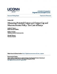
3 Empirical results In this Section, the results of the SVAR model specification are showed. As a preliminary analysis, we estimated different bivariate models by using output and various survey data indicators. Output is defined as the Italian Gross Domestic Product (expressed in euros at constant 1995 prices, seasonally adjusted source ISTAT). The business survey data come from Italian Manufacturing Business Surveys carried out by ISAE. In particular we used data on the degree of plant utilization, on inventories, on the production level and on the confidence climate index1 etc. These data,(except the degree of plant utilization) are qualitative data and are quantified through the balances2. The selection of business survey data to be included in the model was based on their degree of contemporary correlation with the GDP cyclical component obtained with an Hodrick-Prescott filter and on the basis of their stationarity in the sample. Although we tried different specifications in what follows we show the results of the bivariate model including the degree of plant utilization. This variable is able capture the whole economy cyclical dynamics3 with great precision and to match business cycle evolution without introducing phase shifts. The structural model specification, called SVAR, thus includes GDP in log differences and the degree of plant utilization. The lag structure of the reduced form was selected by using the Schwartz and Akaike criteria. The results of the Portmanteau test for the residual autocorrelation do not allow to reject the null hypothesis of autocorrelation absence. The usual heteroscedasticity test indicates omoscedastic residuals. Figure 1 shows the estimated cyclical and trend components alongside with the actual GDP series. The output gap determined through the SVAR specification is positive from the second half of the Eighties till the Nineties and from 1994 to 1996. The end-of-sample cycle becomes more erratic. These findings reflect the stagnation experienced by the Italian manufacturing sector in the past five years.

1

The confidence climate index is obtained combing data on orders level, inventories and production expectations. Balances are built as the difference between positive and negative answers provided by firms. 3 Although the survey data refer to the manufacturing sector, they are able to thoroughly capture the whole economy dynamics (on this point see Hearn and Woitek, 2001 and Cesaroni, 2007). 2

5

Figure 1 Trend/Cycle decomposition SVAR Model 0.0015 12.47 0.001 12.42 0.0005 12.37 0 12.32

-0.0005

12.27

-0.001

12.22

-0.0015

12.17

12.12

-0.002 1985

1986

1987

1988

1989

1990

1991

1992

1993

Trend

1994

1995

1996

1997

P IL

1998

1999

2000

2001 2002 2003 2004

Output gap

4 Data revisions impact A major aspect in the evaluation of a decomposition method performance is the data revision impact on the reliability of the end-of-sample estimates of the trend/cycle components. Indeed, the end-of-sample estimates are subject to revision when new data become available. This updating process generates uncertainty on the real-time estimates that are of the utmost importance for policy-makers’ decisions (van Norden, 1995). To this end in what follows we assess, the stability of the output gap estimates with respect to data revisions. In our analysis, only the revisions due to new data availability are taken into account, while the impact on official data of the uncertainty estimates due to ex post revisions is not considered. This allows to evaluate the effect of the end-of-sample revisions due to new data availability. However, on the basis of the evidence provided by Orphanides and van Norden (1999), the effect of National Accounts revisions on the output gap estimates should not be significant. The reliability of real-time estimates is evaluated by quantifying the impact of 9-step-ahead data revisions on the output gap estimates referred to 2002 Q4. The revisions are computed with respect to 9 quarters starting from 2003:1 to 2005:1 using the following formula: ( y t / t +T − y t / t +i ⋅ 100 )

(18)

where y t / t +T indicates the estimates at time t, including only the information available at time t+T and y t / t +i indicates the estimates in t, obtained through the information available at t+i with i