EUROPEAN ECONOMY EUROPEAN COMMISSION DIRECTORATE-GENERAL FOR ECONOMIC AND FINANCIAL AFFAIRS
ECONOMIC PAPERS
ISSN 1725-3187 http://europa.eu.int/comm/economy_finance
Number 248
May 2006
Proceedings from the ECFIN Workshop "The budgetary implications of structural reforms" - Brussels, 2 December 2005 Edited by S. Deroose, E. Flores and A. Turrini (Directorate-General for Economic and Financial Affairs)
Economic Papers are written by the Staff of the Directorate-General for Economic and Financial Affairs, or by experts working in association with them. The "Papers" are intended to increase awareness of the technical work being done by the staff and to seek comments and suggestions for further analyses. Views expressed represent exclusively the positions of the author and do not necessarily correspond to those of the European Commission. Comments and enquiries should be addressed to the: European Commission Directorate-General for Economic and Financial Affairs Publications BU1 - -1/13 B - 1049 Brussels, Belgium
ECFIN/001324-EN ISBN 92-79-01189-8 KC-AI-06-248-EN-C ©European Communities, 2006..
Preface Most of the reforms discussed within the framework of the Lisbon strategy will benefit public finances in the long term. However, in the short-term, there could a trade-off between some structural reforms and budgetary discipline. This possible tension between reforms and fiscal discipline was identified by academic economists as a possible drawback of the Stability and Growth Pact since its inception. As a result of the 2005 reform of the Stability and Growth Pact, the EU fiscal framework now contains elements that allow better taking into account the budgetary impact of structural reform. These provisions permit to modulate the implementation of the Stability and Growth Pact in case of major structural reforms both in the preventive arm (the definition of medium-term budgetary objectives and the adjustment towards them) and in the corrective arm of the Pact (the Excessive Deficit Procedure). In the coming months and years, ensuring an implementation of the Stability and Growth Pact that takes appropriately into account structural reforms will be a major challenge. The Council Regulations codifying the reform of the Stability and Growth Pact define conditions under which structural reforms could be considered in the EU fiscal framework. However, there are aspects open to judgement by the Commission and the Council. Adequate knowledge about the interactions between structural reforms and public budgets will be crucial for an economically sound use of this judgement. Unfortunately, to date there has been relatively little research on the relationship between structural reforms and government accounts. The workshop “Budgetary implications of structural reforms” organized on 2 December 2005 by DG ECFIN of the European Commission aimed at filling this gap. This issue of the DG ECFIN Economic Paper series collects the papers presented at the workshop. Some of the papers (Andersen, Giorno, Hoeller and Van den Noord) focus on the budgetary impact of structural reforms over the long term and analyse the long-term implications for public finances of policies aimed at reforming social security or the functioning of markets via equilibrium modelling techniques. These papers highlight how the impact of structural reforms on the future path of government budget balances and debt is driven by the interaction between the specific design of the reform, the functioning of the tax system and the social security system, and the overall macroeconomic environment. Other papers (Deroose and Turrini, Roeger) focus on the impact of structural reforms on budgets over the short and medium run. Reforms may hurt budget balances because implying a direct cost in terms of higher expenditures or lost revenues. The most relevant example is that of pension reforms shifting funded pillars outside the government sector. However, indirect costs could arise if political resistance to reforms is countered to some degree by a compensation of interest groups via tax cuts or targeted increased expenditure. These papers aimed at measuring the impact of different types of reforms on public budgets via modelling or econometric techniques. Finally, there are papers (Duval, Heinemann) attempting to answer the question whether the pursuit of budgetary discipline could be a deterrent for structural reforms. The aim is to test the widely quoted argument that a tight fiscal stance reduces the “political capital” available to governments, thereby reducing the feasibility of policies that encounter opposition from interest groups. The analysis in this case is not on the impact of reforms on budgets but, the other way round, on the impact of the fiscal stance on the probability of reforms.
i
The analytical approaches differ across the papers, as well as the datasets employed. This poses an issue in deriving across-the-board conclusions. Nevertheless, a tentative summary of the main common findings can be made as follows. First, many reforms imply considerable potential longterm gains for public finances. However, the size of the impact depends crucially on the design of the reform and the overall economic environment. Second, although the existence of short-term costs of long-term beneficial reforms cannot be easily dismissed, the magnitude of the short-term budgetary impact varies considerably depending not only on which sector of the economy is reformed (e.g., labour market reforms versus pension reforms) but also on the specific design of the reform (e.g., parametric pension reforms versus systemic reforms introducing mandatory funded schemes recorded outside government). Third, the impact of the budgetary situation and the fiscal stance on the likelihood of structural reforms is not clear-cut. The evidence seems consistent with a possible trade-off between fiscal consolidation and labour market reforms, but such trade off is not visible for other type of reforms (product market reforms, financial market reforms, pension reforms).
ii
THE BUDGETARY IMPLICATIONS OF STRUCTURAL REFORMS A Workshop organised by the European Commission Directorate General for Economic and Financial affairs Brussels, 2 December 2005 Centre Borschette 36 rue Froissart, 1040 Brussels
Programme: •
Chair: E. Flores Gual
9.30-10.00
Registration and welcome coffee
10.00-10.15
Opening: Director General K. Regling (European Commission)
10.15-11.45
Session 1: The long-term budgetary impact of structural reforms
•
T. M. Andersen (University of Aarhus, CEPR, CESifo and EPRU) and L. Haagen Pedersen (The Welfare Commission): "Assessing sustainability and the consequences of reforms"
•
P. Hoeller, C. Giorno and P. van den Noord (OECD): "Nothing ventured, nothing gained: the long-run fiscal reward of structural reform" − Discussant: D. Costello (European Commission)
11.45–13.15 Session 2: The transitory impact of structural reforms on government budgets •
W. Roeger (European Commission): “Assessing the budgetary impact of systemic pension reforms”
•
S. Deroose and A. Turrini (European Commission): “The short-term budgetary implications of structural reforms: evidence from a panel of EU countries” − Discussant: R. Beetsma (University of Amsterdam and CEPR)
13.15–14.15 Lunch
iii
14.15–15.45
Session 3: Structural reforms and government budgets: is there a trade-off?
•
F. Heinemann (ZEW): "How distant is Lisbon from Maastricht? The short-run link between structural reforms and budgetary performance"
•
R. Duval (OECD): "Fiscal positions, fiscal adjustment, and structural reforms in labour and product markets” − Discussant: L. Jonung (European Commission)
15.45–16.00
Coffee break
16.00–17.00 Policy panel: Structural reforms in the implementation of the revised Stability and Growth Pact. •
J. Marin-Arcas (ECB), P. Mills (Ministry of Finance, France) and M. Buti (European Commission).
iv
Assessing fiscal sustainability and the consequences of reforms∗ Torben M. Andersen University of Aarhus CEPR, CESifo and EPRU
Lars Haagen Pedersen Welfare Commission
January 24th, 2006
Abstract The paper evaluates fiscal sustainability by use of an explicit intertemporal (OLG) model. Sustainability problems are measured in terms of the needed tax changes which either on a period-by-period basis balance the budget or on a permanent basis ensure that the intertemporal budget constraint is fulfilled. The pros and cons of these approaches to assessing fiscal sustainability are discussed. In an application for Denmark the two metrics for the sustainability problem are calculated and the implications for the design and evaluation of policy reforms are discussed.
∗ Comments and suggestion by the discussant D. Costello and participants at the workshop "The Budgetary Implications of Structural Reforms" are gratefully acknowledged.
1
1
Introduction
The medium to long run developments of public finances is in focus in many countries due to changing demographics. Increasing dependency ratios imply that systematic fiscal deficits may develop, and this raises questions concerning both the sustainability of public finances and thus current policies as well as the timing and scaling of reforms. For short run evaluations of the fiscal position it is important to have a forecast of medium to long run developments, since the former need not be a good indicator for the latter. For EMU countries the GSP stipulates norms for the fiscal position. Originally these were formulated in terms of the current budget and debt position (the 3% deficit-to-gdp and 60% debt-to-gdp norms) with an objective of ensuring that the structural deficit is in balance or surplus. In a recent reinterpretation (ECOFIN council (2005)) it is stressed that the evaluation of the budget position should take the medium to long run developments into account. In particular the influence of demographic changes should be considered. Moreover, it is stressed that the evaluation of the short run position should be seen in perspective of eventual structural reforms leading to more sustainable public finances. Often fiscal policies are evaluated by considering the structural budget balance and questioning whether this is consistent with stabilization of a given debt level. Although readily applicable this approach has some shortcomings. First, in a forward looking perspective the primary balance may change significantly even for a given structural unemployment rate e.g. due to changing demographics. Second, the approach is not easy to apply in evaluating the effects of reforms. Finally, the issue of fiscal sustainability is more complex than just stabilization of debt levels. While it is sensible to consider the medium to long run developments in public finances in order to evaluate the fiscal stance and the need for reforms, it also raises a number of questions. A key question is concerned with reliability and credibility. What is needed is a realistic projection of the development in public finances rather than desired paths. The latter are easy to formulate but do not provide very useful guidelines for an evaluation of the sustainability of current policies. This is in particular important since a main task is to provide indicators on the need and scale of structural reforms as an input to policy discussions. Structural issues are involved in the discussion of possible policy reforms and to this end an explicitly formulated intertemporal general equilibrium model is a useful tool. The framework thus allows for indicators of the fiscal sustainability problem but also for assessment of reforms which may either be phased in over several years or have effects which unfold over a sequence of years. Clearly the specific results depend on the precise modelling assumption which needs to be carefully considered in each separate case. A forward looking approach is needed to take into account expected future developments affecting public finances. In this paper we present a forward looking approach using an OLG model for assessing the sustainability of public finances and thus of current policies. 2
We present metrics by which to assess the sustainability of public finances. A straightforward indicator can be constructed by projecting the future path of public budgets and how it is affected by various reforms. This is useful in particular if the underlying budget profile has a trend, e.g. a systematic tendency towards deficits. However, it is not without problems to project a path with "unchanged policies" in an fully specified intertemporal general equilibrium model, and it is also often hard to interpret a given budget position in terms of the needed scale for reforms. Accordingly, it is useful to translate the sustainability problem into a readily interpretable indicator which can be directly controlled by politicians. This provides a better impression of the order of magnitudes of the needed policy reaction. Via sensitivity analysis it is possible to assess the uncertainty involved. A simple indicator of the need for reforms can thus be calculated by finding the change in e.g. a tax instrument (defined on a broad tax base) needed to balance the budget period by period. Note that this metric has no normative implications as to whether the appropriate policy response is a tax increase. Evaluating how this indicator is affected by a given reform proposal provides a measure of the contribution of the reform to ensure sustainable public finances. Moreover, sensitivity analysis can be performed straightforwardly. The periodby-period indicator suffers from two shortcomings. First, it leaves a number of indicators — one for each year - and not a single and easily interpretable indicator. Second, by implicitly requiring budget balance on a period-by-period basis, it disregards the possibility that variations in the budget position may not necessarily pose a problem (smoothing), and in some cases be part of a reform package (e.g. if it is phased in over a transition period). These problems are overcome by calculating an indicator of fiscal sustainability given by e.g. the permanent change in a tax instrument needed to ensure that the intertemporal budget constraint of the public sector is fulfilled - the sustainable tax rate. By evaluating how this indicator is affected by various reform proposals, a measure can be derived on the overall contribution to an improvement in public finances without concern for the particular timing of the budgetary consequences. A further advantage of this indicator is that it allows a smoothening of the effects over time, i.e. it allows for budget variation over time, but ensures sustainability of public finances (the intertemporal budget constraint is satisfied). The shortcoming is that it may suppress the underlying time profile, and this provides important insights into the process of designing reform proposals. As we will argue below these two indicators are closely related, and the application will show that it is useful to apply both metrics since this provides more detailed information on the mechanisms affecting fiscal sustainability, and also the appropriate way of designing reforms. To assess the robustness and risk profile of the evaluation of the sustainability of public finances it is important to perform sensitivity analysis. This can easily be done by either of the two indicators. The paper presents both of these indicators and shows applications by use of an OLG-model for the Danish economy (the so-called DREAM-model, which is 3
a CGE-OLG model). We present an assessment of the sustainability of current policies and show that there is a substantial sustainability problem despite the fact that Denmark currently has a budget surplus. Since there is an underlying trend deteriorating public finances, this case brings forth the weaknesses and strengths of both indicators. We also present assessment of the implications of three types of reforms (retirement, tax and labour market reform) and discuss aspects to be taken into account in designing reforms. The paper is organized as follows: Section 2 presents a short overview of different approaches to assess the sustainability of fiscal policies. The approach taken in this paper is presented in section 3, and section 4 provides information on the analysis performed for Denmark. The results on fiscal sustainability are presented in section 5. Section 6 discusses reform strategies and presents an evaluation of reform proposals, and section 7 provides a few concluding remarks.
2
Approaches in assessing fiscal sustainability
The concept of fiscal sustainability can be defined in different ways, but the most widespread interpretation is "the government’s ability to indefinitely maintain the same set of policies while remaining solvent" (Burnside (2004, ch. 2 p1).Various approaches and methods have been proposed in the literature to assess the sustainability of fiscal policy. They all depart from the identify linking changes in public debt to the primary balance and debt servicing (all measured relative to gdp), dt+1 = (1 + rt )dt − bt
(1)
where r is the interest rate (growth corrected rate of return), d denotes debt and b the budget balance (revenues less expenditures) relative to GDP. Steady state conditions For given interest rates, growth rates etc. this identity provides a relationship between the debt level (d∗ ) and the primary balance (b∗ ) which can be sustained in the long run (steady state). From this, one can from a targeted debt level infer a required level for the primary balance, or vice versa from a given primary balance infer the implied debt level (provided stability). This approach leads to the so-called primary gap indicator (see e.g. Blanchard(1990)) which gives the difference between the current primary balance and the level needed to sustain a given debt level. The fiscal norms of the GSP pact can also be interpreted from this perspective since a debt level of 60% of GDP can be maintained by a primary deficit of 3% of GDP provided that the growth corrected real rate of return is 5%. Debt dynamics: It is well-known that the stability properties of the debt level depends on the real rate of interest being less than the growth rate. Endogenizing interest determination allows for the possibility that the stability condition depends on the debt level. This implies that there may be threshold levels for public debt below which the system remains stable. Identifying the threshold and comparing 4
current debt levels to the threshold yield an indicator for the sustainability of fiscal policy (see e.g. Tobin and Buiter (1976), Zee (1988) and Bagnai (2004))1 . Both of the approaches mentioned here share the property that they are relatively simple and therefore also easy to apply. However, they rely on rather mechanical assumptions concerning e.g. primary balances, and the forward looking elements in the approach are mainly captured by the dynamics implied by the debt accumulation equation allowing no role for future changes in conditions impinging on public revenues and expenditures. Furthermore, it is very difficult to asses the consequences of structural reforms especially if the reforms due to either implementation lags or effect lags only show their effects gradually over time. Empirical methods An approach to empirical test of fiscal sustainability was proposed by Hamilton and Flavin (1986) and has since been extended by various authors into a VAR framework (see e.g. Carriero, Favero and Giavazzi (2005), Polito and Wickens(2005)). The basic idea is to test for stationarity of primary balances and debt levels. If unit roots in the primary balance or debt levels can be rejected it is not possible to reject the hypothesis that the intertemporal budget constraint for the government will be fulfilled2 . Leaving aside econometric problems concerning the problems of unit root tests (sensitivity to alternatives close to a unit root) the main shortcoming of this approach is that it is backward looking and thereby completely disregards the forward looking aspects currently raising concerns of sustainability in many countries. These methods may be useful in characterizing historical periods but cannot be used to assess future consequences of say demographic changes and the consequences of proposed reforms. Intertemporal approaches Recently a number of analysis have taken explicit outset in the intertemporal budget constraint. Most well-known is generational accounting (see e.g. Auerbach et.al. (1999), Kotlikoff (1995). The basic idea is to use the intertemporal budget constraint in combination with estimations of the contribution rates of currently living generations to calculate the tax burden resting on future generations. By comparing the latter to the burden on newborns the inter-generational profile can be evaluated. Obviously this calculation is based on various assumptions, but it is straightforward to make sensitivity tests to variations in the underlying assumptions. An alternative closure is to consider the permanent decrease in government spending or the permanent increase in taxes to restore generational balance (see e.g. Cardarelli et.al. (2000)). 1 The IMF method of critical debt levels also falls into this category. The aim is to determine threshold levels for the debt level] (public or foreign) which would trigger a "crisis", see e.g. IMF(2003). 2 An alternative method is to test for how primary surpluses respond to public debt, since a sufficient condition for sustainability is that an increase in debt leads to higher budget surpluses, cf Ballabriga and Martinez-Mongay (2005). See Turini(2005) for an evaluation of the short-term budgetary effects of structural reforms.
5
This is related to the so-called OECD approach which also relies on the intertemporal budget constraint but which for a finite horizon solves for the needed adjustment given an assumed level of debt at the end of the period (Blanchard(1990)). The latter property of the method introduces a large element of arbitrariness in the analysis since the results are very sensitive to the imposed time horizon and the stipulated debt level3 . From the abovementioned forward looking approaches it possible to calculate the level at which e.g. taxes need to be to ensure that the intertemporal budget constraint is fulfilled4 . The latter is often motivated by reference to tax smoothing arguments. One shortcoming of these approaches is that they neglect general equilibrium effects of say changes in taxes. This is a serious shortcoming in evaluating both the order of magnitude of the needed changes to ensure fiscal sustainability and the implications of various types of reforms. The second generation approach5 to which the present paper belongs is thus based on an explicit intertemporal general equilibrium model (here: an OLG model for Denmark, cf below). The main attraction is that this approach is formulated in such a way that it can be used directly in the process of formulating and assessing policy proposals.
3
A forward looking method using an OLG model
The purpose is to develop indicators making it possible to assess the sustainability of current policies, and in the case of sustainability problems the order of magnitude of the required reforms. The following outlines the basic mechanisms. A simple model in the appendix illustrates the calculation of the indicators and their relation, while later sections present applications for Denmark. Denote the primary budget deficit - revenues less expenditures - (relative to GDP) by b(xt , yt , zt ) (2) where x denotes a vector of endogenous variables, y a vector of policies, and z a vector of exogenous variables (including foreign variables, demographics, shocks etc.). The endogenous variables are determined by some model left unspecified here for simplicity, but the endogenous response of various variables and how they impinge on the public budget is of course central to the whole approach, cf below. Policies are given by 3 However, for a sufficiently far-sighted horizon the sensitivity wrt. the debt level may be very limited. 4 Frederiksen (2001) proposes a method to calculate the sustainable budget balance given the intertemporal budget constraint and assuming a exponential form for the deterioration in net tax receipts. A disadvantage of this approach is that the sustainable budget balance under a sustainable policy is not time invariant. 5 Heide et.al. (2005) make an assessment of fiscal sustainability for Norway using a CGEmodel and solving for the PAYG value of the pay-roll tax. See also Fehr, Jokisch and Kotlikoff (2004) and McMorrow and Roeger(2004).
6
yt = ft (xt , zt, θt )
(3)
which depend on the current state, the policy form (captured by the function f ) and the policy parameters θ. This representation allows a treatment of both structural and parametric reforms. Hence the public budget is for given policy functions defined by the implicit function β t (xt , zt, θ t ) ≡ b(xt , ft (xt , zt, θ t ), zt ) The public debt level relative to GDP evolves according to dt+1 = (1 + rt )dt + bt
(4)
where r is the growth corrected effective real rate of interest on public debt. The intertemporal budget constraint for the public sector reads6 P V (bt ) − d0 ≥ 0
(5)
where P V denotes the present value operator and d0 the initial debt level. Obviously the budget constraint - both the static and the intertemporal - are fulfilled for a infinity of policies, and it is therefore necessary to put more structure on the analysis to arrive at usable results. The issue is to clarify policies which are sustainable in the sense that they do not violate the intertemporal budget constraint. Passive policies A frequently asked question is what the consequences would be of maintaining unchanged policies. Specifically, how would the public sector budget balance(b) and public debt (d) evolve in the absence of any policy initiatives? While it may be illustrative to show a divergent path for public debt, this approach has two major shortcomings. It is very difficult to determine critical levels for the public budget balance and debt level beyond which the situation is no longer tenable7 . Theoretical work teaches us that the actual path followed by the economy depends critically on the expected future policy interventions used to correct a crisis situation. This is well-known from e.g. the literature on the contractionary effects of expansionary fiscal policy 8 and the so-called "balance-of-payments-crises" literature9 . Empirical work also leaves it unclear what the critical levels are. Moreover, the purpose of discussing sustainability is not to clarify for how long policies can be maintained without provoking a major crisis, but to aid in policy planning so as to avoid the possibility of such crises. 6 Assuming
the usual no-Ponzi restriction. the approach taken by e.g. IMF discussed in section 2. 8 See e.g. Bertola and Drazen (1989) and Sutherland(1993). 9 The "balance of payments crises" literature shows that the crises caued by unsustainable policies will depend on the nature of the policy intervention, which in turn critically would affect the timing of the crises. 7 cf
7
The purpose of an evaluation of fiscal sustainability is to assess the need for policy reforms. Such an evaluation naturally takes its outset in current or unchanged policies, that is, the purpose is not to predict future developments, but to create an informed basis on which to discuss the need and nature of reforms. Leaving aside the practical problems of defining what is meant by unchanged policies, cf below, there is the fundamental problem that a fully specified intertemporal general equilibrium model necessarily builds on the premise that the intertemporal budget constraint of the public sector would have to be fulfilled. That is, an instrument for adjustment needs to be specified to close the model. This property should not be mixed up with Ricardian equivalence since it follows from a consistent modelling of all interrelationships - the attractive property and disciplining device of formulating an explicit intertemporal general equilibrium model. To illustrate this point note that in a standard OLG model Ricardian equivalence does not hold, however, this does not imply that there is no intertemporal budget constraint for the public sector. A pragmatic way of solving this problem is to close the budget by assuming a lump sum transfer in the far future, cf below. This would allow debt to accumulate and make it possible to assess the consequences of "passive" policies. While a pragmatic solution, this approach is not without its problems. The expectations of agents would differ between a case where the budget constraint is fulfilled by an outside transfer and a case with a future lump sum tax increase. However, this problem may have less importance for the path in the initial periods Pay-as-you go A simple constraint to impose on the analysis is to require a balanced budget on a period-by-period basis. Requiring that the total balance is zero for all future periods, i.e. b(xt , yt , zt ) − rt dt = 0 for all t (6) This ensures an unchanged debt position, i.e. dt = dt+1
for all t
Clearly this condition can still be fulfilled for an infinite of combinations of the policy instruments, and it is not immediately clear from (6) what order of magnitudes should be attained by policy changes aiming at ensuring that the condition holds. Clarity can be gained by choosing one instrument (say θ1 ) and solve for the value of the instrument ensuring that (6) holds leaving the policy functions and all other policy parameters constant and thus time-invariant. This approach yields a time dependent value of the policy parameter θpayg (t) 1 which ensures that (6) is fulfilled. The relation and path of θpayg (t) relative 1 to the current value of θ1 (0) yields a perspective on the need and order of magnitude of future policy changes as well as the underlying time profile. If there is a systematic difference between θ1 (0) and θpayg (t), current policies are 1 not sustainable if θpayg (t) is systematically above (below) θ1 (0) and θ1 is a tax 1 (expenditure) instrument.
8
Note that the particular choice of instrument θ1 has no implications for the optimal policy choice. It is obvious that it in general cannot be optimal to let one policy parameter to carry the burden of adjustment. The interpretation is thus that by focusing on one policy instrument one provides perspective on the direction and order of magnitude of the needed policy changes, and one policy instrument is singled out only for simplicity. For this to be useful the instrument θ1 chosen needs to be a general policy instrument which is easily controllable. For instance a tax rate with a broad tax base. In practice a combination of policy instruments will be used, and the requirement is that the package achieves a total effect corresponding to the effect captured by the difference between θpayg (t) and θ1 (0). 1 This approach is relatively simple to apply but it has two main disadvantages. First, it implies that the initial debt level is kept constant throughout time. This leaves aside whether this is optimal. Second, requiring a period-byperiod balancing of the public budget is unnecessarily restrictive and implies that the capital market is not allowed to be used to smooth the adjustment. Sustainable policies An alternative procedure is to solve for the permanent level to which θ1 would have to be adjusted for the intertemporal budget constraint (5) to be satisfied - allowing all policy functions and all other policy parameters to be unchanged and thus time invariant10 . Denote this value by θe1 . The interpretation is thus that by making an adjustment of the policy parameter θ1 to θe1 , the total policy package is sustainable in the sense that it is consistent with the intertemporal budget constraint. By implication future policy changes are only needed to deal with unanticipated changes. The case of sustainable policies can also be interpreted as smooth policies in the sense of time invariant policies. It is often a policy objective to avoid policy changes and having policies invariant over time and thus generations. There can also be efficiency arguments for choosing smooth tax policies (Barro(1979)). By comparing the current value of the policy instrument θ1 to the sustainable value θe1 one can assert both the sustainability of current policies and the needed order of adjustment to ensure sustainability. Specifically we have that current policies violate (14) and therefore are unsustainable, that is, the present value of revenues falls short of the present value of expenditures including initial debt if θe1
θe1
> θ1 < θ1
∂b >0 ∂θ1 ∂b f or 0) then there is a sustainability problem if the sustainable value exceeds 1 1 0 Presuming
that a solution exists, cf also appendix.
9
the initial value, θe1 > θ1 (0), and vice versa for an expenditure instrument ∂b ( ∂θ < 0). 1 If there¯ is a sustainability problem a metric of the problem is given by ¯ ¯ ¯ ¯θ1 (0) − θe1 ¯. An advantage of this approach is that it yields an answer to the question of fiscal sustainability in one metric taking into account the whole future profile of public finances and using capital markets to smooth effects across periods. Notice that this simplicity is attained at the cost of being unable to unravel the profile of the underlying problem from the indicator. The sustainable value of the policy parameter can be interpreted as the present value of the path calculated under the PAYG solution, i.e. θe1 = P V (θpayg (t)) 1
which holds exactly if initial debt is zero, as shown in the appendix. The sustainability indicator obtained by the approach outlined above can be interpreted as a market test of the sustainability of public finances. This is so since the indicator is based on the intertemporal budget constraint given market interest rates, and therefore provides an answer as to whether current policies (policy functions f and parameters θ) are consistent with the intertemporal budget constraint. If the answer is confirmative the conclusion is that it is feasible to maintain current policies. However, this does not answer the question whether it is desirable not least optimal to maintain current policies11 . It is obvious that optimal policies cannot be derived solely by considering the budget constraint. If it is found that current policies are unsustainable it can be concluded that an adjustment eventually would have to take place - current policies cannot be maintained, but the analysis does not say anything about how and when the change will take place. The budget implications of the sustainable tax rate can be calculated by solving for ´ ³ β t xt , zt, (θe1 , θ2 .......θ N )
which gives that the path the primary budget balance would have to follow in order for policies to be sustainable. Note that this path for the primary budget is both dependent on the particular instruments used in calculating sustainable taxes and time dependent. This points to the fact that it is not easy to use a budget metric as a guideline for formulating medium term objectives for fiscal policies. However, as shown in the application below it may be useful to consider the path for the budget balance when discussing the appropriate policy response, cf below. In conclusion, by calculating both the PAYG-tax and the sustainable tax one arrives with the taxonomy that the former implies a constant level for the public debt (and public balance) and a time varying tax rate, while the latter has a constant tax rate and a time dependent level for public debt and the 1 1 Floden(2003) shows in a model with infinitely lived household how the optimal policy prescribes tax smoothing and a pre-funding due to demographic shifts.
10
public balance. In this way the two approaches span two orthogonal dimensions of possible reform directions.
4
An application for Denmark
The following provides an application of the approach outlined above for Denmark.
4.1
The DREAM model12
The analysis is conducted using a large scale dynamic CGE model, named DREAM, which has been developed with the purpose of evaluating mediumto-long term effects of fiscal policy in Denmark. This model is thus quite appropriate for assessing issues of fiscal sustainability and to evaluate the sensitivity to changes in key variables. The model is based on an overlapping generation structure, and the focus is on demographic developments and the Danish public sector. DREAM represents a small open economy with a fixed exchange rate regime, perfect mobility of capital and residence based capital taxation, implying that the nominal interest rate is given by the international capital market. Danish and foreign products are considered imperfect substitutes in both production and consumption, and foreign trade is modeled using the Armington approach. Prices and wages are therefore influenced by internal Danish economic developments. The core of DREAM is the household structure. The model uses the detailed projection of the Danish population presented in section 3.1. The adult population is divided into 85 generations, each consisting of cohorts in a 1-year interval, starting with people who are 17 years of age. For each generation a representative household is constructed. Children are distributed between the households according to the age-specific fertility rates of the demographic forecast. Each representative household optimizes its labour supply, consumption, and savings decision in each period given perfect foresight. Savings take place in owner-occupied dwellings, financial assets (stocks and bonds) and labour market (second pillar) and private (third pillar) pension schemes. The labour market is characterized by unionized behavior giving rise to structural unemployment. There are two private production sectors: a construction sector and a sector producing other goods and services. Firms optimize intertemporally and use labour, capital and materials in the production process. Investments are subject to convex costs of installation, giving rise to gradual capital adjustments. Like the labour market, product markets are characterized by imperfect competition. An exogenous Harrod-neutral, labour-augmenting productivity growth rate of 2 percent annually and an exogenous foreign inflation rate of 2 percent are assumed. 1 2 The Danish Rational Economic Agents Model. For details see Knudsen, Pedersen, Petersen, Stephensen and Trier (1998,1999) and Pedersen, Stephensen and Trier (1999). More information can be found at www.dreammodel.dk.
11
The public sector produces goods that are mainly used for public consumption. In addition it levies taxes and pays transfers and subsidies to households and firms. These are modeled in great detail to capture actual systems and rules as closely as possible. The most important taxes in terms of revenue are local- and central-government income taxes, VAT, excise duties, corporate taxes, property taxes and a tax on yield of pension funds. Tax rates are assumed to remain constant in the forecast period. On the expenditure side 23 different transfers are distinguished and paid out to individuals of each respective age, gender and origin group following the actual distribution in 2001. In the same way expenditures for individual public consumption (mainly educational, health and social expenditures) are distributed to individuals. These individual (per age, gender and origin group) expenses are forecasted to increase with the rate of inflation and the exogenous productivity growth. The remaining collective public consumption is assumed to grow at the same rate as domestic GDP.
4.2
Unchanged policy
The starting point is to evaluate the sustainability of current policies, and this requires a precise clarification of what is understood by unchanged policies. This is complicated since it involves both current tax, transfer and welfare schemes. The key assumptions made here are the following( further details are given in Velfærdskommissionen (2004, 2005)) * Transfer incomes are regulated annually by wage increases in the private sector13 . * The frequency of the population receiving various income transfers is constant across gender, age and country of origin. * The frequency of the population using various forms of welfare services (individual collective consumption) is constant across gender, age and country of origin. The average cost per person is regulated annually by the sum of productivity increases and inflation equal to wage increases. * Collective public consumption is a constant fraction of GDP. * Public investments are determined such that the capital-labour ratio in public production is constant. * All tax rates (including excise taxes) are assumed constant. Taxes levied on a per quantum basis are regulated by inflation14 . * Working hours and the fraction working part time are constant Broadly interpreted the assumptions made here correspond to assuming un1 3 According
to Danish indexation rules"satsreguleringsloven" all transfers are indexed on private sector wages. However, 0.3 percentage points of the wage increase are transferred to a public fund "satspuljen" if wage increases exceed 2%. The funds accumulated in "satspuljen" are to be used for initiatives in the form of transfers or services benefitting recipients of transfer income. Note that since transfers are taxable income the distribution of part of the funds via "satspuljen" rather than by full indexation of transfers tends to deteriorate public finances. 1 4 Currently there is a so-called tax-stop freezing all tax rates, also some at a nominal level (taxation of houses). In the projections the tax-freeze is assumed to be lifted in 2011.
12
changed welfare arrangements and mode of financing via various forms of taxation. The basic question is thus whether these policies can be sustained, i.e. are they consistent with fiscal sustainability.
4.3
The demographic projection
Demographic projections depend on future fertility, mortality and migration. The uncertainty associated with the projection of each of these determinants is significant, and the evolution of the total population becomes highly uncertain in longer run projections. However, what really matters in relation to fiscal sustainability is the robustness of the demographic dependency ratio with respect to changes in the underlying population flows. The analysis is based on the demographic forecast of the Welfare Commission (2004). Using the methods suggested by Lee and Carter (1992), Haldrup (2004) estimates age and gender specific mortality rates for Denmark using data from 1900-2002. These estimates imply that the average annual future growth rates in life expectancy are in the range from 0.08 to 0.09 years for both men and women. However, these estimates are cautious and imply that the growth rate in life expectancy remains approximately half of that projected for Western Europe over the next 50 years (United Nations, 2004). In any case, this suggests that uncertainty with respect to life expectancy may be significant.
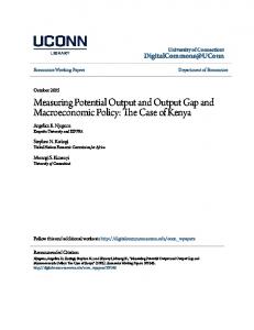
Figure 1: Demographic dependency ratio 2001=100 135 130 125 120 115 110 105 100 95
20 01 20 06 20 11 20 16 20 21 20 26 20 31 20 36 20 41 20 46 20 51 20 56 20 61 20 66 20 71 20 76
90
Note: Persons age group below 15 and above 64 as a fraction of age group between age 15 and 64. Source: Velfærdskommissionen (2004)
The projection shows a fall in the size of the population (from 5.4 million
13
today to 5.0 million in 2070), and the number of working-age persons (15-64) is reduced by 10 per cent from 2002 to 2040 and by 16 per cent from 2002 to 2080. Over the same two periods, the number of elderly citizens (65+) increases by 52 per cent and 47 per cent, respectively. Consequently, the demographic dependency ratio increases by 27 per cent from 2002 to 2040 and by 28 per cent from 2002 to 2080, cf figure 1. This indicates that the increase in the dependency ratio during the next 35 years is not a phenomenon that is isolated to the echo effects of the large post-war generations. Rather, it is a permanent shift to a higher level15 .
5
Fiscal sustainability
We start by presenting the path for public expenditures and revenues under unchanged policies, cf figure 2. It is seen that expenditures gradually but steadily increase to a level systematically above revenues16 .
Figure 2: Public expenditures and revenues 60,0 % of GDP
58,0 56,0 54,0 52,0 50,0 48,0 2003
2013
2023
2033
2043
Expenditures
2053
2063
2073
Revenues
Source: Velfærdskommissionen (2005d) 1 5 Compared to previous yet very recent demographic forecasts, the shift in the dependency ratio is qualitatively different. In the 2001 forecast, the dependency ratio has a global peak around 2040, but the ratio is then reduced to a level which is in between the current level and the peak in 2040. This suggests that the demographic ageing problem has both a temporary and a permanent component. The current demographic projection implies that the ageing problem is almost entirely a permanent phenomenon, see e.g. Andersen et. al. (2005). 1 6 Note that deposits into private pension funds are deductable in taxable income, the return is taxed (at a low rate), but withdrawals are also taxable income. Since there has been a substantial build-up of pension funds since the late 1980s this implies that there is a substantial deferred tax payment in current pension funds. Therefore, the average tax share increases, despite unchanged tax rates.
14
The primary balance is initially in surplus but will gradually deteriorate, and systematic deficits will develop. The budget position changes by 4 percentage points of GDP between now and 2040. Since the change in the demographic dependency ratio is permanent, there is a persistent deficit.
Figure 3: Public finances - Primary and total balance 4,0
% of GDP
2,0 0,0 -2,02003
2013
2023
2033
2043
2053
2063
2073
-4,0 -6,0 -8,0 -10,0 -12,0 Primary balance
Total balance
Source: Velfærdskommissionen (2005d)
The path shown in figure 3 raises the question of whether it is consistent with fiscal sustainability. Are current surpluses and reductions in public debt sufficient to cope with the projected deficits? In the following the base tax rate is used as the instrument for evaluating the needed adjustments to ensure fiscal sustainability. This tax rate is chosen because it is a tax rate with a very broad base (90% of all taxable persons pay this tax, and the tax base is approximately 50% of GDP - the current rate is 5.5%) and easily interpretable. Note that in calculating the level of the base tax in accordance with the PAYG-criterion or for the sustainable tax rate, the consequences of tax changes are taken into account. For the base tax rate the marginal costs of public funds in the DREAM model are 1.67.
5.1
Pay-as-you go solution
A natural starting point is to assume a pay-as-you-go financing where policy is continuously adapted to ensure a balance between revenue and expenses, cf (6). This ensures that the debt to GDP ratio remains constant (consolidated public debt at 5 % of GDP in 2003). Under PAYG financing, the consequences of the demographic changes are financed on a period-by-period basis. This implies that capital markets are not
15
used to smooth the financial burden, cf above. The upward trend in the dependency ratio causes an upward trend in the tax rate on labour income which in the medium to long run becomes more than twice the current level, cf. figure 4. Underlying the trend there are some variations. Initially there is scope for some tax reduction but eventually the demographic development requires an increasing tax rate.
Figure 4: PAYG-tax 16,00 14,00 12,00
%
10,00 8,00 6,00 4,00 2,00 0,00 2003
2013
2023
2033
2043
2053
2063
2073
PAYG-tax Source: Velfærdskommissionen (2005d)
5.2
The sustainable tax rate
Consider alternatively the once and for all change in the tax rate that ensures fiscal sustainability, cf above. More specifically this gives the permanent change in the tax rate which ensures that the intertemporal budget constraint for the public sector is fulfilled. The sustainable tax rate is 7.9 percentage points above the current rate. This shows two things. First, current welfare arrangements are not fiscally sustainable despite current surpluses. Second, the needed reforms are substantial since they should have budgetary consequences equivalent to an increase in the base tax rate by 7.9 percentage points. Since there is an underlying trend in the dependency ratio, it is an implication of the sustainable tax rate that it implies a substantial consolidation of public finances. That is, it implies a pre-funding strategy (for a further discussion see Andersen, Pedersen and Houggard Jensen (2005))17 The primary 1 7 McKissack
and Comley (2005) consider pre-funding strategies adopted in some OECD
16
budget balance would thus remain positive for a long period of time (to 2076), cf figure 5, implying an accumulation of public wealth reaching more than 100% of GDP, which can be used to finance the upward expenditure drift in the future (cf also figure 7 below).
Figure 5: Primary balance - sustainable tax and no reform 4 3
% of GDP
2 1 0 2003 -1
2013
2023
2033
2043
2053
2063
2073
-2 -3 -4 Sustainable tax
No reform
Source: Velfærdskommissionen (2005d)
To underline that other modes of financing are available note that the permanent reduction in public expenditures ensuring fiscal sustainability is about 3.2% of GDP. The permanent increase in private employment is about 270.000 persons equivalent to an increase in employment by 10%. Note that this is a hypothetical number since it is not based on any explicit policy initiatives. Both of these measures also imply a consolidation and are therefore also prefunding or savings strategies.
5.3
Comparison of PAYG-solution and sustainable taxes
PAYG-financing stabilizes the debt ratio but implies a time-varying tax rate with an upward trend, whereas the sustainable tax is constant, cf giure 6. Hence, there is a substantive consolidation of public finances under the sustainable tax. This reflectss the smoothing properties of the prefunding strategy. However, in the present context the smoothing is primarily of an underlying upward trend in the PAYG-tax rather than temporary variations around a more constant level. countries.
17
As a consequences the sustainable tax implies a substantial pre-funding with a substantial wealth accumulation in the public sector. F ig u re 6 : S u s ta in a b le ta x v s . P A YG -ta x 16 ,0 0 14 ,0 0 12 ,0 0
%
10 ,0 0 8 ,0 0 6 ,0 0 4 ,0 0 2 ,0 0 0 ,0 0 2 00 3
2 01 3
20 2 3
20 3 3 P A Y G ta x
2043
2053
2 0 63
2 0 73
S u s t a in ab le ta x
Source: Velfærdskommissionen (2005d)
The paths for public debt implied by the various strategies are seen from figure 7. The PAYG-tax keeps debt at the initial level,and the sustainable tax leads to an initial accumulation of substantial wealth in the public sector. This wealth is used to finance net-expenditures in the far future. F ig u re 7 : P u b lic n e t-w e a lth : N o re fo rm , P A YG -ta x a n d S u s ta in a b le ta x 175,0 125,0
% of GDP
75,0 25,0 -25,02003
2013
2023
2033
2043
2053
2063
-75,0 -125,0 -175,0 N o reform
18
PAYG
S us tainable tax
2073
Source: Velfærdskommissionen (2005d)
Although the prefunding strategy smoothens taxes over time, it also implies a generational profile for the tax burden. This is so since the tax payments for a long period of time (before 2080) would be larger under the prefunding strategy compared to the PAYG-strategy. Considering the taxes paid by a given generation it follows that all generations born before 2030 will have to face a larger tax payment compared to PAYG-financing, and vice versa for generations born after 2030, cf figure 818 . The choice of strategy has the largest implications for generations born between 1970 and 2000. For these generations the present value of the difference corresponds to 0.2 million Dkr per person over lifetime. The gain to generations born after 2060 under the prefunding strategy has a present value of about 0.1 million Dkr per person evaluated over life time.
Figure 8: Difference in net-payments across generations: Sustainable vs PAYG tax 0,25 0,2 0,15 0,1 0,05 0 19 35 19 45 19 55 19 65 19 75 19 85 19 95 20 05 20 15 20 25 20 35 20 45 20 55 20 65 20 75
-0,05
-0,1 -0,15 Note: Present value of the difference in tax payments depending on the year of birth, million Dkr per person Source: Velfærdskommissionen (2005d)
The distribution of gains and losses in net-contributions to the public sector can approximately be used to assess the relative change in utility for each generation. This is so since the effects on wages and prices of the two financing strategies are fairly similar compared to the differences in tax payments. Basically, the prefunding strategy implies that current generations are worse off 1 8 This calculation is based on an earlier analysis, Velfærdskommissionen (2004). There is, however, no qualitaty difference between the two.
19
compared to future generations19 .
5.4
Sensitivity and risk
The calculations presented above apply to the base scenario, but various assumptions can of course be discussed. Moreover, it is important to identify the risk factors which may affect public finances the most. It is therefore important to perform a sensitivity analysis. The results of such sensitivity analyses are given in table 1 in terms of the changes in the sustainable tax rate. Similar analyses can easily be done for the PAYG-tax but are left out here to economize on space. Table 1. Sensitivity — changes in the base tax rate under various alternative assumptions Change in base tax Base scenario 7.9 Demographics UN growth in life expectancy Increased fertility (from 1.7 to 1.8) +5000 immigrants annually - more developed countries +5000 immigrants annually - less developed countries
16.7 8.6 7.9 11.2
Welfare services and leisure 0.10% reduction in work time per year extra 0.15% real growth in welfare service per year
1.0 15.6
Labour market Higher labour force participation descendants from less developed countries
6.2
Interest rate and growth 0.5 percentage points higher interest rate 0.5 percentage points higher growth in TFP
4.8 14.0
Health care "Year to death" and age dependency "Year to death" and age dependency + increasing standards
7.3 14.5
Source: Velfærdskommissionen (2005d).
In the following we shall comment on two particular important aspects of the sensitivity analyses. 1 9 See Jensen et.al.(2002) for a comparison of equivalent variation measures and generational accounts in the DREAM model. The analysis suggests a similarity in relative changes but differences between the two measures occur primarily due to differences in discount factors and the effects of bequest.
20
4.1 Demographics It is seen that the sustainable tax rate is very sensitive to longevity. With no increases in expected life span, the sustainable tax is only marginally above the current rate (1.6 percentage points) while in the base case the difference is 7.5 percentage points. Under UN projections implying about the double growth in life expectancy the tax increase needed is about 16.7 percentage point. This shows how sensitive public finances are to changes in the balances between the number of years a person is net-contributor to the financing and the number of years as net-beneficiary. Note that the projections are made under an assumption of unchanged eligibility ages for early retirement and pensions. This shows that a major part of the financing problem arises from the need to deal with the fact that future generations would have higher longevity than current generations. Table 1 also shows that changes in fertility would only have a minor effect on the sustainable tax rate, whereas it would obviously have some effect on taxes under PAYG-financing. Increased fertility worsens the sustainability problem because future generations are expected to live longer. Permanent changes in immigration only have marginal long-term effects on the demographic composition of the population. Critical for the effects on the financing problem is the labour market attachment of immigrants and their descendants20 . This is so since universal welfare arrangements in Denmark provide entitlements to (almost) all individuals and compensate for lack of income, whereas financing goes via taxes levied on income generated in the market. Assessed from current experiences with the labour market performance of immigrants, it follows that increased immigration from highly developed countries would hardly affect the sustainable tax rate. A permanent increase in immigration from less developed countries would worsen the sustainability problem due to the low employment frequency of this group. If their employment possibilities could be improved, it would clearly contribute to lowering the sustainability problem. Finally, increased emigration could worsen the sustainability problem, in particular since the emigration propensity is larger for highly educated. Currently, return migration is at a high level, but to the extent this changes, the sustainability problem worsens. In short this is so since an investment is made in education, which is not paid back later in the form of tax payments arising from employment. In sum, public finances are vulnerable if immigration is by groups with low employment rates and emigration is by the better educated. Continued globalization must be expected to lead to increases in migration flows, although immigration can be affected politically. Growth It is often hypothesized that growth will automatically create more leeway in public finances. Accordingly, proposals for structural reforms strengthen2 0 Labour force participation is 85% for males and 76% for females. For immigrants from more developed countries the corresponding figures are 69% and 57% and from less developed countries 59% and 41%.
21
ing growth are often also seen as measures to improve public finances, cf e.g. ECOFIN Council (2005). This type of reasoning is based on the fact that budget positions are very sensitive to the underlying business cycle situation. Despite this, the relationship between growth and public finance in the medium to long run may differ. As seen from table 1, increasing the growth rate for productivity growth by 0.5 percentage points the sustainable tax increase is 12.8 percentage points rather than 8.7 percentage points in the base case, i.e. the sustainability problem is worse when the growth rate is higher. This result may at first seem counterintuitive but it arises from some very basic mechanisms, cf also appendix. To see this start with the following basic effects of growth for public finances. If productivity increases in the private sector and wages and income increase, it will have a direct effect on public revenues. However, expenditures will also be affected. There are basically two types of public expenditures, namely wage expenditures and income transfers. The former will over the medium to long-run have to follow wage developments in the private sector21 . The latter will also, under the political distributional constraint that all groups should share the gains in material well-being (or equivalently the distribution of income is not to change), follow wage developments in the private sector. Hence to a first approximation public expenditures will grow in parallel to the growth rate for given welfare arrangements. Actually, there are mechanisms implying that increasing growth may deteriorate public finances. First, since some tax bases are defined on past income (say the taxation of withdrawals from pension funds) it follows that revenue is not following the growth rate22 . Second, increasing growth may lead to increases in the demand for leisure (non taxed) but also increasing demand to standards in services provided by the public sector (expenditure increase) implying a further deterioration of public finances. For the sustainable tax rate there is a further effect at stake. Even under assumptions ensuring that the PAYG-tax is independent of the growth rate. The reason is the trend increase in the dependency rate. The increasing dependency ratio implies a tendency towards systematic deterioration of public finances. The sustainable tax requires that all - current and future generations - pay the same tax rate, such that the intertemporal budget constraint holds. This implies that current generations with lower income than future generations are going to contribute to the financing of future expenditures. The larger the growth rate, the larger the tax rate would have to be to ensure that current generations contribute sufficiently to the financing of expenditure drifts caused by a trend increase in the dependency ratio. The basic budget implications of changes in productivity growth under both PAYG-taxes and the sustainable tax rate are worked out in a simple two-period overlapping generations model presented in the appendix. The mechanisms through which growth affects either indicator are shown to demonstrate why 2 1 Transfers 22 A
are indexed to wages,cf the so-called "satsreguleringslov". similar effect is found for Norway in Heide et. al (2005).
22
increasing productivity growth under very general assumptions may worsen the sustainability problem.
6
Assessing the effects of reforms
The two alternative modes of assessing the fiscal sustainability problems also capture a fundamental dimension of reform strategy, namely a gradual adjustment vs a front-loading/pre-funding(savings) strategy. The sustainable tax corresponds to a pre-funding strategy since the underlying demographic developments have a clear upward trend. Therefore, this implies a considerable consolidation of public finance over several decades. There are several arguments against pursuing a strict pre-funding strategy. First, it implies that current generations come to contribute to the financing of a net-expenditure drift primarily caused by increased longevity of future generations. This is questionable on equity grounds. Second, the needed amount of pre-funding necessarily depends on the base projection. Substantial uncertainty is involved, and it is therefore difficult apriori to determine the needed pre-funding. Finally, on political economy grounds it is hardly advisable to pursue a policy path with substantial budget surpluses and accumulation of public wealth over a prolonged period which at the same time requires the policy discipline that standards in public provision (both services and transfers) should be kept unchanged relative to the base scenario. For these reasons the following considers reform elements which have the property that they are timed so as to match the underlying trends, i.e. they can be considered as parts of a gradual adjustment strategy. The following focuses thus on ensuring a profile for public finances such that the primary budget balance in trend is close to zero. Although some smoothing is allowed, there is no substantial pre-funding or front-loading. While the assessment of the sustainability problem in terms of needed tax changes has served the purpose of clarifying the need for reforms, this does not have any implications for the instrument choice. The reform proposals considered below aim at increasing labour supply and employment. The underlying demographic profile leads to an absolute decline in labour supply, and public finances in Denmark are as noted above very sensitive to the fraction of the population in employment. This is so since employment affects both public revenues (via tax payment) and expenditures (via transfer, since most non-employed have an entitlement to an income transfer in the Danish welfare system). By increasing the employment share of the population it is possible to ensure a financial basis for existing welfare arrangements without resorting to expenditure cuts or tax increases. The following presents two specific reforms - retirement and labour market reform - as well as a complete reform package recently proposed by the Welfare Commission (Velfærdskommissionen (2005d)).
23
6.1
Retirement
A retirement reform can be seen as a natural response to increasing longevity since it directly aims at ensuring a balance between the number of "contributing" and "benefitting" years to the social contract. However, demographic shifts come gradually, and it is a further political concern that eligibility ages for early retirement and pensions are not changed significantly over short periods of time. To allow agents to adapt to the changes it is thus a premise that the changes should be phased in over a longer period of time. Given the long transition period it is interesting to analyse how such changes, which have marginal short run effects over time, will affect public finances and thus contribute to the solution of the fiscal sustainability problem via an increase in labour supply and employment. In Denmark there is an early retirement scheme making retirement possible from the age of 60 (the scheme has incentives to postpone retirement to 62), and the official pension age is 6523 . The average retirement age is currently slightly above 61, and more than 60% have left the labour market before they reach the age of 65. Given the increasing longevity there has been much focus on measures to increase the retirement age. In the following, we present an assessment of a retirement reform with the following two main elements * The early retirement scheme is phased out over the period 2009 to 2028 , specifically the eligible age for entry into the scheme is increased by 4 months per year starting in 2009, and the scheme is closed when the early retirement period becomes 1 year. * The eligible age for public pension is linked to longevity, specifically by increasing the age limit by one month per year starting in 201324 Note that longevity according to the demographic projection underlying the calculations presented above approximately increasing by one month per year. Hence, the reform of the public pension is to index the eligible age to longevity25 . In the assessment of this reform two issues are particularly important. The first is how large a fraction of persons currently on early retirement in the absence of this scheme would be entitled to a different transfer like disability pension. Various assessments of this issue have been made, and it is estimated that between 10% and 30% of those currently on early retirement would be entitled to a different transfer. In the assessment presented here the fraction is 2 3 Eligibility to the scheme requires that contributions have been paid for at least 25 years of the last 30 years. The contribution finances between 1/3 and 1/4 of the accumulated value of the early retirement benefit. The transfer is 91% of maximal unemployment benefits. By postponing early retirement from the age of 60 to 62 there is a higher transfer (100% of maximum unemployment benefits) and a more favourable treatment of some forms of pension savings. Moreover, there is a tax-free bonus to persons delaying early retirement. 2 4 Observe that the indexing of the eligibility age for the public pension is started later than the out-phasing of the early retirement scheme since the opposite would imply a transition period in which the early retirement period would increase. 2 5 At regular intervals the indexation parameter should be adjusted to updates of demographic projections.
24
set at 20%. Second, increasing labour supply by changing retirement schemes is only of interest if it leads to more employment. It is a fact that there is somewhat higher unemployment for elderly in the labour markets. Analyses documented in Velfærdskommissionen (2005b,c) show that this is likely to be driven by mechanisms on both the demand and supply side arising up to the relevant horizon of labour market participation. Hence, by changing entitlement ages, it is to be expected that there somewhat higher unemployment will remain, but the age groups for which this prevails will be shifted upward along increases in the retirement age. The effects of the reforms on labour supply and public finances (primary balance) are given in figure 9 and 10, respectively. The gradual introduction of the changes implies that the immediate effects are modest. For the indexation of the eligibility age for public pension the effect is moderate for a long period since it takes time for the indexing to accumulate to a significant increase in the "pension age". However, eventually both reform elements have substantial effects. It is thus an important implication that a reform which does not change the rules in the very short run and therefore fulfills the political criteria of a gradual change in the entitlements of individuals leads to substantial effects on the sustainability problem. Measured by the effect on labour supply and employment the effect in 2040 is about 160.000 (an increase of 8 %), and for the primary balance there is an improvement in 2040 of 2.1 percentage points of GDP, and the sustainability problem is reduced by some 80%.
Figure 9: Retirement reform - labour supply effect
10,0
%
8,0 6,0 4,0 2,0 2078
2073
2068
2063
2058
2053
2048
2043
2038
2033
2028
2023
2018
2013
2008
2003
0,0
Note: Growth in labour force relative to base scenario Source: Velfærdskommissionen (2005d)
The fact that the retirement reform only has marginal short run effects but substantial effects over the medium to long run points to implications for policy design. This is caused by the political constraint of avoiding sudden and abrupt changes in entitlements . The credibility of the future changes are thus important both from the perspective of individuals but also from a macroperspective.
25
It is therefore important that the changes are institutionalized by explicit indexation and an announced "tablitta" for changes in entitlement ages (early retirement and pension). An alternative procedure which plans to carry out the adjustment in steps by only undertaking one small step in the near future and leaving further steps for an unspecified future will not fulfill this requirement. F ig u r e 1 0 : R e tir e m e n t r e f o r m - b u d g e t e ff e c ts 3 ,0
Perc.point of gdp
2 ,5 2 ,0 1 ,5 1 ,0 0 ,5
78
68
63
58
53
48
43
73
20
20
20
20
20
20
20
20
38
33
20
23
18
13
08
28
20
20
20
20
20
20
20
03
0 ,0
Note: The change in the primary balance (relative to GDP) relative to base case Source: Velfærdskommissionen (2005d)
6.2
Labour market reform
Consider next a reform aiming at reducing structural unemployment. Specifically, the reform includes a shortening of the duration of unemployment benefits (from 4 to 2.5 years), an extended "youth package" implying a stronger focus on education and making it more difficult to enter the social security scheme and with more focus on activation. These ingredients will reduce the structural unemployment rate by 1 percentage point. By linking a change in the structural unemployment rate to explicit policy measures this also sheds light on the general question concerning the importance of unemployment for public finances. The effects on employment and the public budget balance can be read from figure 11 and 12.
26
Figure 11: Labour market reform - labour supply effect 1,2 1
%
0,8 0,6 0,4 0,2 2078
2073
2068
2063
2058
2053
2048
2043
2038
2033
2028
2023
2018
2013
2008
-0,2
2003
0
Note: Growth rate of labour supply relative to base case Source: Velfærdskommissionen (2005d)
Figure 12: Labour market reform - budget effects
0,4 0,3 0,2 0,1 0,0 -0,1
20 03 20 08 20 13 20 18 20 23 20 28 20 33 20 38 20 43 20 48 20 53 20 58 20 63 20 68 20 73 20 78
perc.points of GDP
0,5
-0,2 Note: Change in the primary balance (relative to GDP) relative to the base case Source: Velfærdskommissionen (2005d)
6.3
Reform package
The Welfare Commission (Velfærdskommissionen (2005d)) has recently proposed a reform package to solve the sustainability problem. The main thrust of the package is to increase labour supply and employment so as to provide a sound financial basis for welfare arrangements without resorting to tax increases or savings. The package has the following main ingredients; i) a retirement re27
form (cf above), ii) a labour market reform (cf above) iii) an education reform, iv) an integration reform and v) a tax reform. The main focus of all reform elements is to improve public finances by a strengthening of labour supply and employment, although the various reform elements have been chosen also with other concerns in mind. As noted this focus takes its outset in the fact that there will be a downward trend in labour supply..
Figure 13: Labour supply - no reform 2800 2700 1000 persons
2600 2500 2400 2300 2200 2100 2000 2003
2013
2023
2033
2043
Reform package
2053
2063
2073
No reform
Source: Velfærdskommissionen (2005d)
The reform package has a substantial effect on labour supply and employment with an effect in 2040 of 252.000 equivalent to an increase by 10% in the labour force relative to the "no reform" path. The contribution of the various reform elements is shown in figure 14.
28
Figure 14: Employment effect - decomposition on reform elements 12,0 10,0 8,0
%
6,0 4,0 2,0
20 03 20 08 20 13 20 18 20 23 20 28 20 33 20 38 20 43 20 48 20 53 20 58 20 63 20 68 20 73 20 78
0,0 -2,0
Education
Labour market
Integration
Retirement
Tax
Source: Velfærdskommissionen (2005d).
The reform package implies that the deteriorating trend in public finances is eliminated and sustainability ensured. While the initial favourable position is used to further consolidate public finances, the package essentially implies that the primary balance is projected to vary very closely around zero reflecting that the net-effect of the overall reform package is timed so as to counteract the consequences of the demographic changes. The budget balance is projected to be very close to zero (maximum deficit in any year is 0.5% of GDP) and net-debt relative to GDP is in no year above 10% of GDP. The reform package is thus neither a pure PAYG-solution nor a pure consolidation/pre-funding strategy, although if anything it is closer to the former than the latter26 . 2 6 Note that in the long run there is a tendency towards budget surpluses leading to some consolidation coping with problems in the very long run. This has litlle current policy relevance since it applies to a very long horizon.
29
Figure 15: Primary balance with and without reform 4,0 3,0
% of GDP
2,0 1,0 0,0 -1,02003
2013
2023
2033
2043
2053
2063
2073
-2,0 -3,0 -4,0 Without reform
With reform
Source: Velfærdskommissionen (2005d).
The contribution of the various reform elements to the improvement in public finances is shown in the table below. Table 1: Decomposition of the contribution of the various reform elements to the change in the primary budget position 2005 2020 2030 2040 2060 Base scenario 3.0 -0.1 -1.5 -2.1 -3.4 Education 0.0 0.1 0.2 0.3 0.5 Labour market 0.0 0.4 0.4 0.4 0.4 Integration 0.0 0.2 0.2 0.3 0.3 Retirement 0.0 0.9 2.0 2.1 2.8 Tax 0.0 -1.2 -0.7 -0.6 -0.6 Other reform elements 0.0 -0.3 -0.2 0.0 0.3 After reform 3.0 0.0 0.4 0.4 0.5 Velfærdskommissionen (2005d)
Assessed in terms of fiscal sustainability the reform package solves the problem27 The contribution of the various elements to the fiscal sustainability problem is: i) retirement 82.6% , ii) labour market 14%, iii) education 12.6%, iv) integration 10.4%, while iv) the tax reform worsens sustainability by -21% . The reform package includes one element where the timing plays a very crucial role, namely the tax reform.The tax reform is motivated by both concerns for asymmetries in the existing tax structure as well as the need to make the system more robust to globalization. The particular tax reform considered involves 2 7 Exactly
99.6% of the sustainability problem identified in the base case is eliminated.
30
a shifting of taxes from labour income to real estate (i.e. shifting taxes in the direction of less mobile tax bases). However, increased taxation of real estate would be immediately capitalized in prices causing a capital loss for housing owners on top of the liquidity problem the tax increase may create (in particular for families which have recently entered the market)28 . By phasing in tax reductions on labour income quicker than the tax increase on real estate it is possible both to eliminate the immediate liquidity problem and to moderate the price effect29 . This reform element thus has the element of first deteriorating public finances, but eventually public finances will improve, and the reform can thus be seen as an "investment" in a better tax structure. Note that the packages also includes increase public spending on research (to reach a target for public expenditures on research of 1 % of GDP) and prefunding of pensions for groups not covered by mandatory labour market pension or similar pension scheme. This explains the short span of years for which the primary balance is in deficit, cf figure 15. Since it is an implication of the package that it brings public finances to a situation very close to budget balance, it follows that exposure to various forms of risk is reduced. This applies to variation in the interest rate and the growth rate. For changes in longevity - where increase beyond the relative moderate projections made here may be expected - this only applies if the underlying indexation formula is maintained.
7
Concluding remarks
The issue of fiscal sustainability has been considered in an explicit intertemporal setting, and indicators based on either a period-by-period (gradual) approach or a once-and-for-all (permanent) approach have been considered and applied for Denmark. The framework here allows an explicit consideration of reforms aiming at eliminating the systematic trends towards making the situation fiscally unsustainable. Likewise it is possible to evaluate how reform proposals motivated by other concerns would affect fiscal sustainability. It is an open question over how long horizons policies should be planned. However, it is important to consider the short term position of public finances in relation to medium to long run trends. The current situation for Denmark is a case in point - despite current budget surpluses and a trend decline in public debt, it is the case that current policies are not fiscally sustainable. There is a clear and systematic trend towards deterioration of public finances for unchanged welfare and taxation systems. Since this primarily is driven by demographic changes and a substantial lead time is needed to make changes in retirement and pensions systems it is necessary to consider public finance over a horizon of non-trivial length if sudden changes in policies should be prevented. 2 8 Note that since the taxation (ejendomsværdiskat) depends on the price development it follows that the liquidity problem is moderated the larger the price effect, and vice versa. 2 9 Evaluated in a partial model the effect is a price reduction of 11%. Taking into account the whole package and the general equilibrium effects, the effect is halfed.
31
Concerns for inter-generational equity and risk both point in the direction of ensuring that the budget balance over the medium to long run is fairly close to zero. A policy aiming at substantial pre-funding would in a number of respects be a problematic strategy. By keeping public finances close to balance it follows that the risk exposure is smaller, and the room for accommodating short-run business fluctuations are larger. These points have been illustrated by consideration of a reform package recently proposed by the Welfare Commission (2005d).
32
Appendix A: The welfare state and the social contract - PAYG-financing and sustainable tax rates A simplified version of the social contract can be represented in a standard two-period overlapping generations model with generations in the work force (the young) overlapping with retirees (the old). Nt is the number of persons in the generation being young in period t (and therefore old in period t + 1), a1t denotes per capita services received from the public sector as young in period t, and a2t per capita services received by the old in period t. Pensions paid to old in period t denoted pt . The total income of those being active in period t is denoted y1t , and it is taxed by a proportional tax rate τ . The primary balance of the public sector in period t is bt
= Nt τ t y1t − Nt a1t − Nt−1 (pt + a2t ) = Nt [τ t y1t − a1t − (1 + ρt )(pt + a2t )]
where 1 + ρ is the demographic dependency ratio30 in period t, i.e. 1 + ρt . It follows that ρ is negative when the population is growing, and positive when it is decreasing. An increase in longevity prolongs the "retirement period" and increases the demographic dependency ratio and can thus be interpreted as a reason why ρ is positive. In net terms the exchange of the young generation with the public sector is Γ1t = Nt a1t − Nt τ t y1t and for the old it is Γ2t = Nt−1 (pt + a2t ) Given policy rules for welfare service, pensions and taxes - p(), a1 (), a2 () and τ () - can be realized if and only if P V (b) + D0 ≥ 0
(7)
where D0 is the initial public debt. In the following we consider policy rules where pt a1t a2t
= γyt = α1 yt = α2 yt
(8) (9) (10)
For pensions and welfare services it follows that they are proportional to current income. The first part of this assumption implies a fixed relation between 3 0 The fact that not all working people survive and reach the pensioner stage can easily be included. Denote by Ot the number of pensioners in period t out of generation Nt born in t − 1, where Ot = (1 − φt−1 )Nt−1 , and φ is the likelihood of dying young. The demographic Ot dependency ratio is now N = 1+e ρ ≡ (1−φt−1 )(1+ρt ) < (1+ρt ). Beyond this reinterpretation t of the change in the demographic dependency ratio, the analysis remains unchanged.
33
pensions and income for those working, i.e. gains from growth are distributed equally among active and passive members of society. The second part implies that expenditures on welfare services are proportional to income developments. This reflects that welfare services are labour intensive and that public wages follow private wages very closely.31 Notice that all parameters are assumed to be time-independent, i.e. given rules for pensions and welfare services are considered. The following focuses on the requirements to financing given the increase in the demographic dependency ratio. This is operationalized by considering the changes in the tax rate needed to finance the expenditures. We consider two financing strategies, namely, pay as you go with continuous adjustment of taxes to balance the budget and the sustainable tax rate, which over time is consistent with the government intertemporal budget constraint. We consider a "small and open economy" for which the (real) rate of interest r is exogenous. To simplify, the interest rate is assumed constant over time. Similarly the growth rate g is exogenous and constant over time. It is assumed that r > g, i.e. corrected for growth the real rate of interest is positive.
Pay as you go financing Under pay as you go financing it is a requirement that there is budget balance on a period-by-period basis, i.e.,32 bt = [τ t − α1 − (1 + ρt )(γ + α2 )] y1t = 0
(11)
which immediately implies AY G τP = α1 + (1 + ρt )(γ + α2 ) t
(12)
It follows straightforwardly that the optimal tax rate is increasing over time if the demographic dependency ratio is increasing (ρ > 0) and vice versa. The intuition is that it is necessary to tax the current work force more when a large fraction of the population has to be supported. It is also an immediate implication that Γ1t Γ2t
= Nt a1t − Nt τ t y1t > 0 = Nt−1 (pt + a2t ) < 0
i.e. in net-terms the working population is net-contributors, and the retirees are net-beneficiaries from the welfare arrangements. Note that the tax rate under PAYG-financing is independent of the income level and thus the underlying growth rate. The reason for this neutrality result 3 1 At the same time, demand will pull in the same direction if the income elasticity in demand for welfare service is high. 3 2 Can more generally be translated as a requirement for unchanged debt (relative to GDP). For simplicity, the initial debt is assumed to be zero, and balance in the primary budget will maintain a zero debt.
34
is that all welfare arrangements (services and pensions) and the tax system are proportional to the current income level. Increased growth will thus lead to a proportional income in revenues and expenditures for the public sector and therefore in net-terms not change anything. This neutrality result depends on the way welfare arrangements and taxation have been arranged, which can be seen by considering two special cases. i) The tax system includes tax bases dependent on income in past period, e.g. via taxation of pensions or the return on savings. The budget restriction or the requirement to budget balance is in this case bt = [τ t − α1 − (1 + ρt )(γ + α2 )] y1t + µy1t−1 = 0 where µy1t−1 , is the revenue from taxation related to tax bases dependent on earlier periods’ income (here income in the previous period). The balanced budget requirement can be rewritten £ ¤ bt = τ t − α1 − (1 + ρt )(γ + α2 ) + µ(1 + g)−1 y1t = 0
where g is the growth rate in income (y1t = (1 + g)y1t−1 ). The tax rate under PAYG-financing becomes AY G τP = α1 + (1 + ρt )(γ + α2 ) − µ(1 + g)−1 t
i.e. increased growth will increase the tax rate. The intuition is that while expenditures are increasing proportionally to income, this is not the case for the tax base since it also depends on previous periods’ income. Therefore the needed tax rate to finance given welfare arrangements goes up. ii) Pensions are proportional to earlier labour income, i.e. pt = γy1t−1 In this case pensions are seen relative to the income (and [ this-?] consumption possibilities) while working and not relative to those currently working. In this case the budget restriction becomes £ ¤ bt = τ t − α1 − (1 + ρt )(γ(1 + g)−1 + α2 ) y1t = 0
and the tax rate under PAYG-financing
AY G τP = α1 + (1 + ρt )(γ(1 + g)−1 + α2 ) t
i.e. increased growth will reduce the PAYG-tax. The intuition is that expenditures on pensions are not affected by growth since they depend on last period’s income.
Sustainable tax rates An alternative financing strategy is to keep tax rates constant over time to avoid varying tax rates and possibly minimizing tax distortions (Barro (1979)). The sustainable tax rate is defined as the tax rate b τ , which it is possible to maintain 35
in all periods so as to finance welfare arrangements of the form (8), (9) and (10) and that the intertemporal budget constraint for the public sector is fulfilled, i.e. ¶i ∞ µ X 1 bt+i = 0 (13) 1+r i=0
Initial debt is assumed to be zero. By use of (11 and (13), it is found that the sustainable tax rate b τ , satisfies
¤ 1 £ 0 = [b τ − α1 − (1 + ρt )(γ + α2 )] y1t + τ − α1 − (1 + ρt+1 )(γ + α2 ) y1t+1 b 1+r µ ¶2 ¤ £ 1 + b τ − α1 − (1 + ρt+2 )(γ + α2 ) y1t+2 ...... 1+r
or
" # µ ¶2 1 1+g 1+g 0 = [b τ − α1 ] −(γ+α2 ) (1 + ρt ) + (1 + ρt+2 )...... (1 + ρt+1 ) + 1+r 1+r 1 − 1+g 1+r (14) Consider the special case, where ρ is constant over time. In this case the sustainable tax rate is τ = α1 + (γ + α2 )(1 + ρ) b
It is seen to coincide with the tax rate under PAYG-financing, cf (7). This indicates that differences between the two modes of financing arise when the demographic dependency ratio is not constant over time. It is an implication that the sustainable tax in this case is independent of the interest rate and the growth rate.
Trend changes in demographic dependency ratio Consider a stylized situation with a trend change in the demographic depeni+1 dency ratio given as (1 + ρt+i ) = (1 + ρ) . This implies that the sustainable tax (14) becomes
It follows that ∂b τ ∂ρ ∂b τ ∂g ∂b τ ∂r
τ = α1 + (γ + α2 )(1 + ρ) b
(1 + r) − (1 + g) (1 + r) − (1 + g)(1 + ρ)
"
(1 + r) − (1 + g) (1 + r) − (1 + g) = (γ + α2 ) + (1 + ρ)(1 + g) 2 (1 + r) − (1 + g)(1 + ρ) ((1 + r) − (1 + g)(1 + ρ)) # " (1 + r)ρ = (γ + α2 )(1 + ρ) 2 >0 [(1 + r) − (1 + g)(1 + ρ)] " # (1 + g)ρ (1 + g)(1 + ρ). 36
#
>0
An increasing trend in the dependency ratio increases the sustainable tax rate. For the case where the dependency ratio is increasing (ρ > 0), it follows that an increase in the growth rate increases the sustainable tax rate, as does an increase in the interest rate. The intuition is that the sustainable tax distributes the financing requirements over time. Since increasing growth means increasing expenditures in the future, and since current generations are contributing to the financing it follows that the tax rate has to go up. Similar reasoning applies for the interest rate effect. With a trend in the demographic dependency ratio, the initial budget balance is b0
= [b τ − α1 − (1 + ρ)(γ + α2 )] y1t · ¸ (1 + g)ρ = (γ + α2 )(1 + ρ) y1t (1 + r) − (1 + g)(1 + ρ)
which implies that the sustainable tax rate implies an initial budget surplus if the demographic dependency ratio is increasing, and vice versa if it is decreasing, i.e. b0 > 0 for ρ > 0, and b0 < 0 for ρ < 0. With an underlying trend in the dependency ratio, it follows that the sustainable tax rate causes an initial consolidation to create a financial basis from which to finance future expenditure increases. With an underlying demographic trend, the sustainable tax rate thus induces savings to ensure a constant tax rate over time. With an underlying upward trend in the dependency ratio, it is straightforward to compare the sustainable tax rate with the PAYG-tax rate, since AY G τP t
i.e.
= α1 + (1 + ρ)i+1 (γ + α2 )
τ = α1 + (γ + α2 )(1 + ρ) b
(1 + r) − (1 + g) (1 + r) − (1 + g)(1 + ρ)
· ¸ (1 + r) − (1 + g) AY G i − τ b = α + (1 + ρ) (γ + α ) − α + (γ + α )(1 + ρ) τP 1 2 1 2 t (1 + r) − (1 + g)(1 + ρ) · ¸ (1 + r) − (1 + g) = (γ + α2 )(1 + ρ) (1 + ρ)i − (1 + r) − (1 + g)(1 + ρ) AY G AY G −b τ < 0, and there exists a e t, where τ eP −b τ> It follows that for ρ > 0 : τ P 0 t 0. This shows that the sustainable tax rate smooths the financial burden caused by the trend increase in the demographic dependency ratio.
PAYG-taxes and the sustainable tax rate It follows immediately by use of () defining the PAYG-tax that the sustainable tax from () can be written ¤ 1 £ 0 = [b τ − α1 − (1 + ρt )(γ + α2 )] y1t + τ − α1 − (1 + ρt+1 )(γ + α2 ) y1t+1 b 1+r µ ¶2 ¤ £ 1 + b τ − α1 − (1 + ρt+2 )(γ + α2 ) y1t+2 ...... 1+r 37
or 0 =
and therefore
¤ ¤ £ 1 £ AY G AY G y1t + y1t+1 b τ − τP τ − τP b t t+1 1+r µ ¶2 £ ¤ 1 AY G + τ − τP b y1t+2 ...... t+2 1+r τ= b
¶i ∞ µ X 1+g i=0
1+r
AY G τP t+i
i.e. the sustainable tax equals the present value of the PAYG-tax calculated by the growth corrected real rate of interest. Note that this presumes that the initial debt level is zero.
38
REFERENCES Andersen, T.M., (2005): Social Security and Longevity, CESifo Working paper Andersen, T.M., and R. Dogonowski (2002): Social Insurance and the Public Budget, Economica, 69, 415-432. Andersen, T. M., S. E. H. Jensen, & L. H. Pedersen (2004): The Welfare State and Strategies To-wards Fiscal Sustainability in Denmark, Arbejdsrapport 2004:4 Velfærdskommissionen Arbejderbevægelsens Erhvervsråd (2004a): ”Størrelsen af de fremtidige udfordringer” Auerbach, A. J., and K. Hassett (2001): .Uncertainty and the Design of Long-Run Fiscal Policy, in A. J. Auerbach, and R. D. Lee (eds.) “Demographic Change and Fiscal Policy”, Cambridge Uni-versity Press, Cambridge, UK. Auerbach, A., and K. Hassett (2002a): .Fiscal Policy and Uncertainty, International Finance, 5(2), 229.242. Auerbach, A., and K. Hassett (2002b): .Optimal Long-Run Fiscal Policy: Constraints, Preferences and the Resolution of Uncertainty,.NBER Working Paper 7036, National Bureau of Economic Re-search, Boston, Mass. Bagnai, A., 2004, Keynesian and Neoclaisscal Sutatinability indciators, with applications to emu member countries. Ballabriga, F.C. and C. Martinez-Mongay, 2005, Sustainability of EU public finances, European Commission, Economic Paper 225. Barro, R. (1974): Are Government Bonds Net Wealth?, Journal of Political Economy, vol 82, pp 1095-1117 Barro, R (1979): On the Determination of Public Debt”, Journal of Political Economy, vol 87, pp 940-971 Benz, U. amd S. Fetzer, 2004, Indicators for Measuring Fiscal Sustainability: A Comparative Application of the OECD-Method and Generational Accounting, University of Freiburg. Bohn, H. (2001): .Social Security and Demographic Uncertainty: The RiskSharing Properties of Alternative Policies, in Campbell, J. and M. Feldstein (eds.) “Risk Aspects of Investment Based Sociial Security Reform”, University of Chicago Press, Chicago. Blanchard, O. & S. Fischer (1989): Lectures on Macroeconomics, MIT Press Burnside, C. (2004): Fiscal Sustainability in Theory and Practice, book manuscript, Duke University. Carriero, A., C. A VFAvero and F. Giavazzi, 2005, Fiscal Sustainability: A New Framework for tests and indicators. Dardarelli, R., J. Sefton and L.J.Kotlikoff, 2000, Generational Accounting in the UK, Economic Journal, 110, F547-F574 Det økonomiske Råd (2004): Dansk Økonomi, forår 2004, Copenhagen Diamond, P. (2003): “Taxation, Incomplete Markets and Social Security”, Munich Lectures in Economics, MIT Press. Dimson, E., P. R. Marsh, & M. Staunton (2002): “Thriumph of the Optimists: 101 Years of Global Investments Returns”, Princeton University Press
39
Dixit, A. K. & R. S. Pindyck (1994): Investment underUncertainty, Princeton University Press. Fehr, H., S.Jokisch, and L.J.Kotlikoff, 2004, Fertility, Mortality, and the Developed World’s Demographic Transition, CESifo Working Paper 1326. Flodén, M. (2003): Public Saving and Policy Coordination in Aging Economies, Scandinavian Journal of Economics, 105, 379-400. ECONFIN Council, 2005, Improveing the implementation of the Stability and Growth Pact, Brussels. European Commission, Public Finances in EMU, various issues Finansministeriet (2004): Finansredegørelse 2004, Copenhagen Finansministeriet (2005): Økonomisk Redegørelse, maj 2005, Copenhagen Frederiksen, D., K. M. Heide, E. Holmøy og I. F. Solli, (2004): Makroøkonomiske virkninger av Moderniseret folketrygd, Statistisk Cesentralbyrå, Økonomiske Analyser 5, 60-70. Frederiksen, N.K., 2001, Fiscal Sustainability in the OECD, A simple Method and some preliminary results, Working Paper 2001, no 3, Finansministeriet, Danmrk Gordon, R., and H. Varian (1988): .Intragenerational Risk Sharing, Journal of Public Economics, 37, 185.202. Haldrup, N. (2004): .Estimation af middellevetider for mænd og kvinder i Danmark, 2002-2010, baseret på Lee-Carter metoden,. Arbejdsrapport 2004:3, Velfærdskommissionen. Hansen, N. P., S. E. H. Jensen, and M. Junge (1999): .Government Solvency, Social Security and Debt Reduction in Denmark, in T. M. Andersen, S. E. H. Jensen, and O. Risager: “Macroeconomic Perspectives on the Danish Economy”, chap. 7. Macmillan Press, London, UK. Heide, K.M., E.Holmøy, I.F.Solli and B. Strøm, 2005, Fiscal sustainability problems i a wealthy welfare state: CGE assessments for Norway. IMF, 2003, Sustainability Assessments - Review of Application and Methogological Refinements. Jensen, S. E. H., U. Nødgaard, and L. H. Pedersen (2001): .Fiscal Sustainability and Generational Burden Sharing in Denmark, Nordic Journal of Political Economy, 28(1), 43.60. Knudsen, M., L. Pedersen, T. Petersen, P. Stephensen, and P. Trier (1998): .Danish Rational Eco-nomic Agents Model - DREAM Ver. 1.2,.Working paper, www.dreammodel.dk, DREAM, Copen-hagen. Knudsen, M. B., L. H. Pedersen, T. W. Petersen, P. Stephensen, and P. Trier (1999): .Dynamic Calibration of a CGE-Model with a Demographic Application, Working paper, www.dreammodel.dk, DREAM, Copenhagen. Lack, C. & Kugler, P. (2003): Price Level Uncertainty and Real Interest Rates: An Empirical Investigation, Working Paper Lee, R., and L. Carter (1992): Modelling and Forecasting the Time Series of U.S. Mortality, Journal of the American Statistical Association, 87, 659.671. Lee, R., and S. Tuljapurkar (2001): “Population Forecasting for Fiscal Planning: Issues and Innovations” in Auerbach, A. and R. Lee (eds.): “Demographic
40
Change and Fiscal Policy”, chap. 2. Cam-bridge University Press, Cambridge, UK. Lippman, S., and J. McCall (1981): The Economics of Uncertainty: Selected Topics and Probabilis-tic Methods, in K. J. Arrow, and M. D. Intrilligator (eds.) “Handbook of Mathematical Econom-ics”, chap. 6. North-Holland, Amsterdam. Markeprand, T. L. H. Pedersen, & P. Stephensen (2003): DREAMs disaggregerede befolkningsfremskrivning til år 2100. Resultater og Metode. McKIssack, and B. Comley, "005, Fiscal Sustainability and pre-funding strategies in OECD Countries, Working paper Nielsen, S., and O. Risager (2001): Stock Returns and Bond Yields in Denmark 1922-1999,.Scandinavian Economic History Review, 49(1), 63.82. Nordhaus, W.D., 2003, Comment on A.J.Auerbach, Fiscal Policy, Past and Present, Brookings Papers on Economic Activity, 1, 130-134. Oksanen, H., 2003, population gageing and public finance targets, European Commission, Economic Papers 196 Pedersen, L. H. (2002): Befolkningsudvikling, integration og økonomisk politik, DREAM, Rapport til Tænketanken om udfordringer for integrationsindsatsen i Danmark Pedersen, L., P. Stephensen, and P. Trier (1999): A CGE Analysis of the Danish Ageing Problem,. Working paper, www.dreammodel.dk, DREAM, Copenhagen. Polito, V. and M. Wickens, 2005, Measuring Fiscal Sustainability, Working Paper University of York Regeringen (2000) Et bæredygtigt pensionssystem, Copenhagen, Denmark Turini, A. 2005, The Short-tem budgetary implications of structural reforms: Evidence from a panel of EU countries. United Nations (2004): World Population in 2300. UN, New York. Velfærdskommissionen (2004): Fremtidens velfærd kommer ikke af sig selv. Analyserapport. Velfærdskommissionen, Copenhagen, Denmark. Velfærdskommission (2005a): Fremtidens velfærd og globaliseringen. Analyserapport. Velfærdskommissionen, Copenhagen, Denmark Velfærdskommissionen (2005b): Fremtidens velfærd — sådan gør andre lande. Analyserapport. Velfærdskommissionen, Copenhagen, Denmark Velfærdskommissionen (2005c): Befolkningsudvikling, velstandsdilemma og markoøkonomiske strategier, Teknisk Analyserapprort. Velfærdskommissionen, Copenhagen, Denmark Velfærdskommissionen (2005d),: Fremtidens velfærd - Vores valg, Analyserapport, Copenhagen, Denmark. Wadensjö, E. & C. Gerdes (2004): Immigrants and the Public Sector in Denmark and Germany. I Tranæs, T. &K. F. Zimmermann eds.:”Migrants, Work, and the Welfare State”, University Press of Southern Denmark and the Rockwool Foundation Research Unit
41
NOTHING VENTURED, NOTHING GAINED: THE LONG-RUN FISCAL REWARD OF STRUCTURAL REFORM Claude Giorno, Peter Hoeller and Paul van den Noord OECD, Economics Department, Paris
Paper prepared for the European Commission Workshop: The budgetary implications of structural reforms Brussels, 2 December 2005
42
NOTHING VENTURED, NOTHING GAINED: THE LONG-RUN FISCAL REWARD OF STRUCTURAL REFORM
Introduction ...................................................................................................................................................44 Linking reforms and the budget ....................................................................................................................45 The UK budget: a role model? ...............................................................................................................45 Quantifying the cost of inaction .............................................................................................................47 Quantifying the impact of regulatory reform .........................................................................................51 “Big bangs” and gradualism: the experiences of New Zealand and Australia.......................................51 Structural reform in an empirical expenditure rule .......................................................................................53 Linking structural reform and fiscal performance: what can a macro-model tell?........................................57 Effects of coordinated reform in monetary union ..................................................................................57 Structural reform in a single country in monetary union .......................................................................61 Effects of a decline in structural unemployment with a more active fiscal policy.................................65 Some policy implications ..............................................................................................................................65 Bibliography..................................................................................................................................................68
43
Introduction 1. We take it for granted that fiscal discipline is important: i) fiscal policy volatility can undermine growth; ii) a pro-cyclical policy can destabilise the economy; iii) large deficits and rising debt undermine the long-run sustainability of fiscal policy and iv) excessive deficits will be a burden on future generations (Fatas, 2005). Fiscal rules are one way to cope with such fiscal policy biases, but they need to be underpinned by institutional settings so that they can be enforced at the national, and in the case of the euro area, at the Community level. 2. The EU fiscal framework was set to underpin the single currency. It was designed to address one key concern, namely that once exchange rates within the single currency area ceased to exist, financial markets would not longer discipline fiscal policy. Fiscal profligacy in one country could affect area-wide interest rates and crowd out economic activity in other countries. As interest rate differentials across the euro area countries have become small despite a divergent fiscal performance, there is little evidence of spill-over effects, probably because there is little to crowd out due to persistent economic slack in the large euro area countries. 3. This may be one reason why the arguments in favour of rules-based fiscal co-ordination have shifted towards long-term issues, not least because ageing-related concerns oblige governments to recognise the implications of current budget decisions for public finances in the future. Also, greater weight has progressively been put on the incentives built into budgetary institutions that produce fiscal biases (higher deficits, expenditure and taxes). But, while these institutions have improved to some extent, they are still lagging best practice in many euro area countries. 4. At the same time, calls to make the Pact more flexible have mushroomed. Some were motivated by new member countries’ need to boost infrastructure outlays, against the backdrop of relatively low public debt levels. Some observers have argued in favour of the “golden rule”, along the lines of the one introduced in 1997 in the United Kingdom. 5. Another rationale for a rewrite of the rules, and the topic of this conference, is that structural reform may yield long-term economic gains but entail up-front costs. The estimated gains of structural reforms are usually uncertain, whereas any immediate political and budgetary costs, such as compensation schemes to offset redistributive effects, are felt immediately and more tangibly. Moreover, some reforms will involve J-curve effects; a cut in taxation will reduce budget receipts immediately while effects on incentives to work, save and invest may be slow to materialise. This asymmetry could discourage reforms, especially in a monetary union, where they cannot be supported via an easing of monetary policy. Similarly, a move towards privately funded pension schemes would lead to deficits in the public scheme but initial surpluses in the private schemes as contributors transfer to them. 6. According to the fiscal rules a waiver could be granted under the excessive deficit procedure to countries on the basis of “exceptional circumstances” (EC 2005a). While the Treaty had already stipulated that “other relevant factors” should be part of the “exceptional circumstances”, these were not specified. The revamped Pact decided by the European Council in March 2005 specifies them and the conditions under which they are taken into account. These include a country’s efforts to pursue the Lisbon agenda, to foster R&D or “a high level of financial contributions” to underpin the “unification of Europe” and “international solidarity” (development aid). Consideration would also be given to pension reforms. Concerning the Lisbon agenda, the new Council Regulation observes: “In order to enhance the growth-oriented nature of the Pact, major structural reforms which have direct long-term cost-saving effects, including through raising potential growth, and therefore a verifiable impact on the long-term sustainability of public finances, should be taken into account when defining the adjustment path to the medium-term budgetary objective for countries that have not yet reached this objective and in allowing a temporary deviation from this objective for countries that have already reached it” (EC, 2005b). All these provisions, however, only apply if “an excess over the reference value is temporary” and if the deficit ratio “remains close to the reference value”, as stipulated in the Treaty.
44
7. There is not yet a proper framework for making decisions about such exemptions in place. In this paper, various aspects of the nexus between structural reforms and budgetary developments that should underpin such a framework will be highlighted. In the first part of the paper we look at the following issues: i) to what extent do budgets cost structural reforms? The United Kingdom, which has a very elaborate fiscal framework, is used as an example. ii) There may be budgetary cost from not reforming government programmes, such as disability or early retirement programmes, which should also be taken into account. iii) Large inventories of structural reforms exist. While they have been used to estimate the effects of reforms on growth, budgetary implications are seldom quantified. This is obviously difficult to establish. Two countries, New Zealand and Australia, which have implemented a radical reform agenda are used here to shed some light on these issues. The second part of the paper uses econometric tools to establish to what extent structural reform affects public expenditure, in the short as well as the long run. The data allow us to detect both upfront cost and long-run gains of structural reform, although both seem to be modest in comparison with other structural determinants. The third part uses simulations with the OECD’s Interlink model to highlight the implications of reforms that affect technical progress, the participation rate and the natural rate of unemployment in different settings.
Linking reforms and the budget
The UK budget: a role model? 8. Assessing the budgetary implications of structural reforms in the short, medium and long run is shrouded with many difficulties. In many cases, governments do provide a costing of changes in tax and spending plans and often also beyond the current budget. 1 Obviously, changes in tax and spending plans are pursued for many other purposes than purely fiscal ones. UK Budgets (HMT, 2001, 2002, 2003 and 2004), for instance, provide an assessment of Budget policy decisions over a three-year horizon under the following headings: meeting the fiscal rules and funding public services; meeting the productivity challenge; increasing employment opportunity for all; building a fairer society; a modern and fair tax system; and protecting the environment. 9. Budget 2002 (Table A.I), for instance, lists 54 spending and tax measures and estimates their budgetary effect. The budgetary impact of 16 measures implemented since Budget 2001 are estimated as well. The biggest measure was a payroll tax increase and the second biggest an increase in the generosity of the Child Tax Credit and Working Tax Credit for families with children. All other measures were small, ranging from beer duty relief for small brewers to simplifying capital gains tax. While the list of measures is long, only those are included where the impact of the decisions and circumstances can be quantified with reasonable accuracy. Moreover, spending that is fixed by the spending reviews and embedded in Departmental Expenditure Limits is not included in the Budget costing of decisions. In 2002, the net fiscal impact of the identified spending and revenue measures was nearly 1% of GDP, but considerably lower in most other Budgets. In comparison, the forecasting error for the deficit was equivalent to 1% of GDP for the year-ahead projection in recent years and nearly 1½ per cent of GDP for the two-year ahead projection (Table 1). There is no strong hint in the Budget costings that reforms have generated large budgetary costs in the short term. However, this is so mainly, because the spending underpinning the ongoing reforms to health, education and infrastructure are built into (hence respect) the Departmental Spending Limits.
1. According to the 2003 Survey on Budget Practices and Procedures (available at http://ocde.dyndns.org/), 55% of the OECD countries provide multi-year cost estimates for all new spending items, and another 20% do it for some mandatory spending items. The survey does not cover revenue changes.
45
Table 1. The costing of Budget policy decisions in the UK Budgetary measures as a per cent of GDP1 2001-02 Budget 2001 Measures since Budget 2000 Budget 2002 Measures since Budget 2001 Budget 2003 Measures since Budget 2002 Budget 2004 Measures since Budget 2003
-0.2 -0.3
2002-03 +0.2 -0.4 -0.1 -0.0
2003-04 +0.3 -0.3 +0.6 -0.2 -0.1 +0.1
2004-05
+0.7 -0.2 -0.0 +0.0 -0.1 -0.1
2005-06
2006-07
+0.0 +0.1 +0.0 -0.1
-0.0 -0.1
1. A plus sign indicates an Exchequer yield. Source : HM Treasury, Budget 2001, 2002, 2003, 2004.
10. What this spending has achieved is open to debate, as the new metrics to measure government outputs, following the Atkinson Review, are not yet fully in place. Assessments of feedbacks of tax and spending changes on economic activity are even rarer. HMT’s effects of budget measures, for instance, do not include effects on overall levels of income and spending. This is not surprising, because there is often no consensus on effects. Depending on the underlying model and empirics, a rise in payroll taxes can have a negative short, medium or long-term impact on structural unemployment, or none at all. Effects of R&D tax credits or grants on R&D spending and ultimately growth are notoriously difficult to quantify. Or the effect of savings incentives on substitution between different savings vehicles versus aggregate savings is usually impossible to pin down. And sometimes, long lags imply that any discernible effects of reforms would only show up after many years. Still, in the United States, attempts are underway to include feedback effects in assessing tax and spending proposals (Box 1). Box 1. Dynamic scoring In the United States, legislative proposals are scrutinised by the Congressional Budget Office (CBO) and the Joint Committee on Taxation (JCT). They provide a baseline and forecasts of the changes in expenditure and revenues that would result from proposed legislation over the following ten years.1 The forecasts provide a cost estimate or “score”, for each piece of legislation that is reported by a Congressional committee (Page, 2005). In the past, the scoring was static, not taking into account macroeconomic feedback effects. Dynamic scoring, which is still in its infancy, takes into account induced changes on output, inflation, interest rates or other macroeconomic feedbacks. The scoring is important as it influences how favourably initiatives are viewed in Congress and the Senate. A tax cut, for instance, could raise output significantly, with a large cut in tax rates having little implication for net government revenues. If this feedback is not included, the tax cut will be viewed less favourably by Congress, which is usually constrained to keep the total revenue cost of a tax package within pre-set targets (Altshuler et al., 2005) The outcome of dynamic scoring depends on the models used and on assumptions about macroeconomic policy reactions. In assessing the 2004 budget, forward-looking, life-cycle growth models and more traditional macroeconomic forecasting models were used. For the latter, various monetary policy reactions to the fiscal stimulus were simulated, while the growth models differ in various respects. Given different models and assumptions, the outcomes differed widely. Concerning the JCT’s analysis, incorporating dynamic effects reduced the net revenue cost of one proposal by 6 to 28% over the first five years and 3 to 23% over the second five years. Auerbach (2005) concludes from these first attempts, that “… it seems clear that dynamic scoring analysis has value, but also that adjustments to estimates are smaller than some might have expected. The process to date offers some support to those on both sides of the debate. On the one hand, the ability of CBO and JCT to produce dynamic analyses of complex, realistic proposals lends credence to the argument that dynamic analysis and, indeed, dynamic scoring may be feasible. On the other hand, the many models used and the many assumptions needed leave many with doubts about the quality of these estimates and how they would fit into the budget scoring process as currently structured.” 1.
On the expenditure side, the CBO provides the baseline and the scoring, on the revenue side the CBO provides the baseline and the JCT the scoring.
46
Quantifying the cost of inaction 11. One could argue that, before allowing more leeway under the fiscal rules, unproductive spending should be pruned first, which would probably leave enough room to spend on priority areas, without running up against the deficit limit. Similar issues relate to reforms, or the lack thereof, of budgetary frameworks, which are far from being best practice in many EU countries (Joumard et al., 2004). The design of reforms themselves may also be problematic: perhaps the scope for more cost-effective approaches is not being exploited. There are many examples of government spending programmes that tend to undermine growth, come at a high budgetary cost, sometimes grow considerably faster than GDP and are difficult to reform. They crowd out more productive government spending programmes. As such programmes tend to push countries towards the Maastricht deficit limit, the question arises whether policy inaction in such areas should not be taken into account, when granting greater flexibility on spending in priority areas. 12. The potential sources of fiscal stress built into government programmes are multiple. Fiscal pressures may mount because of biased incentives of government programmes, for example in the case of early retirement and disability schemes. The implicit tax on continued work, which gauges incentives to quit work before the retirement age, is very high in many European countries (Figure 1). There have been reforms, but most were minor, though Italy lowered the implicit tax a lot between 1998 and 2003. Early retirement lowers labour utilisation and has fiscal costs that can amount to several per cent of GDP. Similarly, the number of disability benefit recipients varies considerably across countries and only a few countries were successful in reducing the number of beneficiaries (Figure 2). In fact, in many countries, the number of beneficiaries keeps on rising rapidly. Figure 1. Implicit tax on continued work: early retirement1,2 2003 100 OECD average
90 80
NLD
70
LUX
PRT ESP
60
AUT
50
BEL
FIN FRA
EU
40
OECD average
IRL
30
DEU
NOR
GBR JPN CHE
KOR
SWE
20 CAN
10
AUS
0 0
ITA
USA ISL NZL
10
20
30
40
50
60
70
1. Average of implicit tax on continued work in early retirement route, for 55 and 60 year olds. 2. EU: 15 European countries excluding Denmark and Greece. Source: OECD (2005), Going for Growth, Paris.
47
80
90
1998
100
Figure 2. Income support for disability 1 Share of working age population non-employed and receiving disability benefits (per cent) 1999 14 OECD average
POL
12
10
NOR SWE
8
NLD
BEL USA
AUS
OECD average
GBR
6
DEU FRA
4
ITA
EU AUT
DNK
PRT
CAN
ESP
2 MEX KOR
0 0
TUR
2
4
6
8
10
12
1990
2
14
1. EU: 15 European countries excluding Finland, Greece, Ireland and Luxembourg. 2. 1995 for Austria, Mexico and Poland. Source: OECD (2005), Going for Growth, Paris.
13. There are also cases, were reform efforts have been considerable, but reform outcomes tend to fall short of expectations. Majnoni d’Intignano (2001), for instance, argues that health reforms in France are recurrent, actually close to one every year between 1975 and 2000, but have barely dented spending growth, or have slowed growth in one year, but with a catch-up towards the underlying spending trend the next. The costing of changes in government programmes is not too difficult for programmes that are relatively simple and where at least some changes in policy parameters influence private decision making in a straightforward way: the implications of pension reforms, for instance, have been well researched by the Commission or the OECD. More complex issues, like the effects of health care reforms are much more difficult to quantify. There are many actors and incentive effects are difficult to model. 14. The cost of inaction can be illustrated by resorting to the now fashionable distinction between the Nordic, Anglo-Saxon, continental and Mediterranean social models. Boeri (2002), for instance, compares their performance in terms of meeting three objectives: reductions in income inequality and poverty; protection against uninsurable labour market risk; and the reward to labour market participation. And indeed, geography and economic characteristic tend to coincide. Sapir (2005) uses the same typology, but focuses on efficiency and equity aspects: Efficiency is measured by a high employment rate and equity by a low poverty rate. 15. Figure 3 shows that all Nordic and Anglo-Saxon countries are above average in terms of employment, whereas most continental countries (except Austria and the Netherlands) and Mediterranean countries (except Portugal) rank below average. On the other hand, poverty is relatively high in the Mediterranean and Anglo-Saxon countries and relatively low in the continental and Nordic countries. Sapir (2005) has analysed the reasons for these differences. What is important in the context of this paper is the fiscal sustainability of social models. Net public debt as a per cent of GDP is much lower in the “efficient” countries and much higher in the continental and Mediterranean countries (Table 2). Moreover, debt does not tend to come down much in the high-debt countries (except Belgium), while it has staid low or even come down further in most better-performing countries.
48
Figure 3. European social systems: employment rates and probability of escaping poverty
Source: Sapir (2005).
49
Table 2. Gross and net debt development Change in Gross debt Net debt 1993 2005
Gross debt % of GDP 2005
Net debt % of GDP 2005
61 48 48 66 65
-6 -41 2 -28 39
-18 -4 -11 -32 3
-16 -24 -23 -7 -2
46 30 78
39 .. 46
-3 -65 01
6 .. 201
72 74 100
61 45 90
24 22 -45
33 17 -38
121 53 108
98 31 ..
-51 -14 -2
-31 -10 ..
Nordic model Sweden Finland Denmark Netherlands Austria Anglo-Saxon model United Kingdom Ireland Portugal Continental model Germany France Belgium Mediterranean model Italy Spain Greece
1. 1995-2005 Source: OECD, Economic Outlook No. 77 database.
16. A similar pattern emerges when looking at growth performance and fiscal policy (Figure 4). In the period 1999-2005, trend growth was only 1½ per cent per year on average in the three major euro area countries, but 3¼ per cent in the smaller countries. Faster growth coincides with a strong fiscal performance, while the contrary tends to be true for the slower-growing countries. Econometric work provides evidence that fiscal consolidations are more likely to be undertaken and successful if trend economic growth is high (von Hagen, 2002). At the same time, the smaller fast growing-economies were able to maintain fairly rapid growth in public spending while keeping their government deficits in check. Greece is of course an important exception with soaring spending and a whopping government deficit despite strong growth. Figure 4. Trend growth and fiscal policy
1999-2005 average Cyclically-adjusted balance (% of GDP)
Growth in real current expenditure (%)
5
7 IRL
4
FIN
6
3 GRC
2 1
PRT ESP
NLD
-1 -2
DEU ITA
-3
FRA
FRA
BEL
PRT
2
4
2 1
DEU
GRC
0
FIN NLD AUT
ITA
-4
3
ESP
AUT
-5
4
IRL
BEL
0
5
6
8
0
Growth in real trend GDP (%)
2
4
6
8
Growth in real trend GDP (%)
Source: OECD, Economic Outlook No. 77 database.
50
0
Quantifying the impact of regulatory reform 17. Things become even more tricky when assessing the effects of changes in the regulatory stance on growth and government budgets. The OECD has developed a broad range of indicators concerning the stringency of labour and product market regulations, which are discussed in more detail in Duval (2005) and feed into the econometric exercise in the next section. 2 The OECD has also produced a lot of empirical work that traces the effects of the regulatory stance on employment and unemployment rates, R&D intensity and ultimately growth. This work has culminated in the OECD’s Growth Project (OECD, 2001) and feeds into the ongoing structural surveillance work (OECD, 2005). Substantial methodological progress has been achieved in constructing structural policy indicators with an econometric link to economic performance. 18. Such inventories are potentially very useful, but there are also limitations, when assessing the budgetary implications of structural reforms:
•
These inventories leave out a wide variety regulations, such as health and safety or environmental regulations, which could have a budgetary impact.
•
There is in general no direct link between these inventories and budgetary effects and it would seem difficult to establish the link between reforms and side-payments to get reforms underway.
19. Moreover, while the body of empirical work on growth is enormous, there are still considerable disagreements about what reforms can achieve in the short and long term. In particular, the short-term adjustment costs associated with reforms are under-researched. In addition, results are data-quality, model and estimator dependent. While cross-country growth regressions have been an extremely popular means of testing ideas about the sources of growth, many of the variables claimed to be significant have not stood up to tests for statistical robustness (Ahn and Hemmings, 2000). Another problem is the lack of accepted formal theoretical models that can accommodate the wide range of variables that are often included as explanatory variables, despite advances in the theory of economic growth. A related issue is that causal links between aggregate economic variables and growth are bi-directional, hence most estimates are likely to suffer from endogeneity problems. We are tempted to quote Blanchard (2005) who, after reviewing the literature on whether enough is known about unemployment to give advice to policy makers about how to reduce it, concludes: “I believe we do – with the proper degree of humility”.
“Big bangs” and gradualism: the experiences of New Zealand and Australia 20. Some OECD economies have undergone a radical transformation, with major fiscal implications. New Zealand is a prime example. It initiated quite radical and wide-ranging reforms in the mid-1980s. These reforms encompassed both macroeconomic stabilisation and structural change (Evans et al., 1996). The reforms followed a decade of anaemic growth, which, at less than ½ per cent, was indeed considerably lower than it is currently in the euro area, while inflation was rampant and the government and current account deficits exceeded 6 and 8% of GDP, respectively. 21. Key reforms included financial market deregulation and the granting of operational independence to the Reserve Bank; deep labour market reforms, though they were only enacted from the early 1990s onwards; and telecommunication and electricity reforms. These reforms did not include any side-payments, but there were many reforms affecting the budget directly. Support to manufacturing industries and agriculture was withdrawn, which lowered spending, but also lowered revenues due to hefty tariff cuts on industrial products. Direct government assistance to industry and agriculture declined form 16% of primary government spending to just 4% in 1993/94. At the same time, tax policy put a sharp focus on the neutrality 2. The World Bank has also developed inventories of policy measures. Another example is the indicators developed by the Fondazione Rodolfo Debenedetti.
51
of the tax system: a comprehensive value added tax replaced a myriad of differing sales taxes, while the corporate and income tax base was broadened and tax rates reduced. Tax incentives concerning exports or retirement savings were abolished. On the spending side, focus was put on organisational and managerial devolution and improved accountability, for instance in health and education. Chief executives became responsible for managing departments, being directly accountable to their Ministers for hitting specific output targets. Moreover, the large number of trading departments was turned into state-owned enterprises, many of which were subsequently sold. 22. Stronger growth did not help fiscal consolidation early in the reform era. Partly reflecting heavy industrial and agricultural restructuring and job losses from rapid efficiency gains of former trading departments, GDP barely increased between 1984 and 1991. Also the exchange rate and real interest rate were high. Early in the reforms, consolidation was largely achieved by revenue increases and while some spending items were pruned severely, spending on health, education and social services increased as a per cent of GDP. But stronger growth followed and a fiscal surplus was achieved in the 1993/94 financial year. Fiscal performance has been strong since then, the government recording a deficit in only one year since 1994 and a net debt position of more than 40% of GDP has swung into a net asset position of 10% of GDP currently. This partly reflects a decent, though not outstanding, growth performance and partly the principled approach to fiscal management that was put in place in 1994. It is a blueprint for principles that underpin responsible fiscal management and transparency, which have been taken up in the UK’s code of fiscal conduct and the OECD Best Practices for Budget Transparency. Macroeconomic policy was set to provide stable policies rather than stabilisation policy. 23. Reforms in New Zealand since the mid-1980s were broad ranging and quick, against the background of large macroeconomic imbalances. By tackling many areas quickly there was no stable coalition formed to oppose reforms: for instance, farmers who had their subsidies withdrawn, 3 strongly supported tariff cuts; and farmers and other businesses then put pressure on the government to reduce spending to bring down the interest and exchange rate. But moving quickly also led to some backlashes, as the reform process stalled between 1988 and 1991, from when onward it resumed again. The experience highlights that fiscal consolidation and radical change can go hand in hand, even when the results of reforms on economic performance do not come quickly. 24. In contrast with New Zealand, the Australian reform process was gradual, but it was also principled and coherent (Banks, 2005). As in New Zealand, policy prior to the reforms was characterised by being highly regulated, anti-competitive and redistributive, even though the macroeconomic background, while not brilliant, was more benign. Productivity growth of just over 1% between 1973 and 1990 was relatively poor and, also affected by terms of trade losses, the international income-per-capita ranking slipped badly. Though reforms started in 1973 with a 25% across-the-board tariff cut, this precipitated a heavy backlash against reforms. It took until 1988, that tariff reductions were phased in and virtually all tariffs were below 5% by 1996. The early 1980s also saw financial market reforms. Increased competition led to pressure to reform labour markets and sheltered sectors. The reforms ultimately embraced all product markets, factor markets and the public sector, including as in New Zealand the commercialisation, corporatisation and privatisation of many government enterprises. 25. Contrary to New Zealand, Australia adopted an incrementalist approach to reforms, thus avoiding heavy initial adjustment costs. The programme evolved in a cumulative way to encompass reforms across much of the economy. Moreover, and again contrary to New Zealand, reforms were accompanied by retraining schemes and displaced workers could rely on the relatively generous welfare safety net. Adjustment costs were also eased by sector-specific restructuring and assistance schemes, which amounted to AUD 600 million annually under the Automotive Competitiveness and Investment Scheme. Similarly, when price support for the milk industry was abolished in 2000, farmers were provided with a substantial stream of payments, financed by a levy on milk consumers. Also regional policy schemes eased the 3. The largest farmer association, the Federated Farmers of New Zealand argue that the sudden and unexpected removal of subsidies have made the farming sector stronger and that farmers are determined never again to be dependent upon government handouts (Federated Farmers of New Zealand, 2002). Productivity gains, for instance, moved from 1% pre-reform to nearly 6% post-reform, while the initial impact of the reform, while sizeable, was much milder than officially projected.
52
adjustment blow in some cases. Policy has thus dealt with the front-loaded timing of the potential losses of reforms as well as the fact that costs of reform are often concentrated on particular groups. The reform process had a fiscal cost, but it was limited and easily outweighed by the overall gains: concomitant with the reforms, there was a sharp rise in the trade to GDP ratio and business R&D surged, boosting productivity growth to among the highest in the OECD and the income-per-capita ranking improved from the 15th place in the mid-1980s to the 8th currently. Not surprisingly, fiscal performance improved a lot as well: the general government balance swung from a deficit peak in the early 1990s of more than 6% of GDP into a surplus by 1998 and has staid in surplus since then, except in one year. Net debt will be eliminated in 2006 and a net asset position will build up. 26. Clearly, for both countries the evidence is that the impact of major structural reforms was a major improvement in fiscal performance. Yet, how to apportion the success between a strengthening in budgetary institutions and better growth performance is unclear.
Structural reform in an empirical expenditure rule 27. Since the proof of the pudding is always in the eating, in this section we try to identify empirically the impact of the structural policy stance on public expenditure, using some basic econometrics. The assumption is that countries in which structural policy stances are geared towards greater market flexibility, the efficiency of welfare systems will generally be higher and government involvement in the economic process – be it through regulation or financial support - more effective. At the same time, potential output would be higher and as a result, everything else equal, public expenditure would decline relative to (potential) output. However, there may be short-run offsets in the form of upfront budgetary cost, such as compensation schemes for people losing their job or rents, which tends to raise public expenditure on a temporary basis. 28. The structural policy indicator capturing structural reform efforts referred to here is the one used by Duval (2005). It is calculated as the sum of normalised OECD indicators in five fields (employment benefits, tax wedges, employment protection legislation, retirement incentives and product market regulation). They are displayed in Figure 5; a higher value corresponds to a tighter stance (more rigidity) and vice versa, and a decline in the indicator suggests that “appropriate” structural reforms have been implemented. Countries that stand out by relatively “tight” stances (high value of the indicator) are all European countries. Some of these countries have also implemented major structural reforms in the past decade (notably Spain, Sweden, Denmark, Belgium and the Netherlands), suggesting that poor initial conditions are a good “predictor” of future structural reform (as confirmed by Duval, 2005). This is encouraging and suggests some tendency towards global convergence, perhaps helped by the Lisbon agenda.
53
Figure 5. Aggregate structural policy stance indicator
8 1985-1994 6
standard deviation
1995-2003
4 2 0 -2 -4 -6
standard deviation
Fr a Be l N ld
Ita
Pr t
Irl Au t N or G rc Es p Sw e D eu D nk Fi n
U SA C an Au s G br Jp n N zl C he
-8
29. As in Duval (2005) we consider 21 countries for which we have annual observations for the period 1985-2003. Using this dataset, we estimated the following partial-adjustment relationship:
PRI it = λPRI it −1 + αSTRit + β ΔSTRit +
(1)
∑γ
k k CON it −1
+ δ i + ε it
k
30. In this relationship PRIit is the level of cyclically-adjusted primary expenditure as a per cent of GDP in country i in year t. STRit is the overall structural policy stance. It is included to capture the long-run effect of the structural policy stance on public expenditure. The term ΔSTRit is the change in the structural policy stance indicator which serves to capture any upfront budgetary cost of structural reform - its expected sign is negative as predicted by theoretical models such as that reported in Beetsma and Debrun (2005). CONit-1 is a vector of control variables, δi are country fixed effects and εit is the normally distributed residual. The method used is ordinary least squares. 31.
Following Martinez-Mongay (2002), four control variables have been considered:
•
Per capita gross national income at 2000 purchasing power parities. This captures “Wagner’s law”, which predicts that high-income countries will exhibit higher shares of public spending in GDP than low-income countries owing to a change in preferences in favour of public goods and services such as health care, education and social services. The expected sign is positive.
•
The dependency ratio. Ageing puts pressure on notably health care and pension expenditure, hence a priori one expects public outlays to be higher in countries that portray a high dependency ratio (measured by the share of people older than 65 in the total population). The expected sign is again positive.
•
Trade openness (sum of exports and imports of goods and services as a per cent of GDP). A standard finding in the literature is that more open economies will have bigger governments in order to protect their citizens against cyclical volatility in economic activity. However, it could also be argued that in a globalising world small open economies, due to their greater exposure to international competition, will be under pressure to keep public expenditure low so as to secure competitive gains from a low tax burden. Accordingly, the net effect on government size is ambiguous.
54
•
Public debt ratio to GDP. There is a large body of literature providing evidence that governments whose debt position threatens to become unsustainable will rein in public expenditure (rather than increase taxes which will at best only bring short-term relief). Hence in countries where public debt is high, government size will be negatively affected and vice versa.
32. The type of electoral system is another factor that emerges from the literature as relevant for the size of government (majoritarian voting rules yield smaller welfare systems), but it will not be considered here (or rather this will be picked up by the country fixed effects). Baumol’s “cost disease”, which predicts that as an economy grows the relative price of public services and hence the share of public expenditure in GDP will increase, will be considered as already being captured by the per capita income effect. 33. Before considering the impact of structural policy stances on government size, we look at the explanatory power of the controls (Table 3). European countries generally portray higher primary expenditure ratios, but also tend to score higher on debt, dependency, openness and lower on GDP per capita than for example the United States. This suggests that the control variables are unlikely to be able to explain the bulk of the cross-country variation in primary expenditure. Accordingly, country fixed effects should play an important role, as confirmed by the estimation results. Table 3. Primary expenditure and its standard determinants Primary expenditure ratio (%) 198519951994 2003
Debt ratio (%) 19851994
19952003
Dependency ratio (%) 19851994
19952003
Openness (%) 19851994
19952003
GDP per capita (at 2000 prices and PPP, US$) 198519951994 2003
Australia
31
33
29
30
17
19
35
42
34388
40831
Austria Belgium Canada Denmark Finland
47 43 38 49 47
47 42 35 52 48
58 131 79 74 30
69 122 89 63 58
22 22 15 23 12
23 25 17 23 13
70 134 55 69 52
84 152 78 80 69
33799 31551 33499 34999 30869
40647 38420 38188 41837 36492
France Germany Greece Ireland Italy
46 41 31 35 39
48 43 35 29 39
42 39 74 99 95
67 60 110 51 128
21 22 22 18 21
24 25 27 17 26
43 50 46 112 40
50 59 50 160 51
34517 37342 16521 24755 26902
40164 37164 19717 42852 31696
Japan Netherlands New Zealand Norway Portugal
24 47 40 53 30
28 42 36 55 37
73 86 64 34 65
122 72 40 37 64
17 18 16 15 20
24 19 17 12 23
19 108 56 71 64
20 121 61 72 66
33239 34166 28474 34502 19418
37961 42149 32274 46292 25232
Spain Sweden Switzerland United Kingdom United States
33 56 28 38
32 54 31 37
53 65 36 43
67 72 51 48
20 16 21 24
24 14 22 24
37 61 69 51
54 79 77 56
24358 36600 41653 32993
30583 40637 43892 40808
31
30
68
66
18
19
20
24
44591
52872
EU151 Average
38 39
39 40
62 64
70 71
19 19
21 21
59 60
72 72
27473 31864
33304 38129
Standard deviation
9
8
26
28
3
5
29
35
6670
7219
1. Unweighted average. Source: OECD Economic Outlook 78 database.
55
34. The regression results for the controls, without and with country-fixed effects, are shown in the first two columns of Table 4. The inclusion of country-fixed effects indeed proves to be necessary; without them the significance levels are unsatisfactory except for the debt ratio and the lagged dependent variable. In the equation with country-fixed effects, the regression coefficients for the dependency ratio, per capita income and public indebtedness have the expected sign and are all significant. Trade-openness has a negative sign, and is also significant. 35. The long-run coefficients, which are the more interesting ones to look at, can be computed as γk/(1-λ). Based on this calculation, the long-run semi-elasticity on the dependency ratio turns out to be about ¼, which suggests that if in any country old-age population growth outpaces total population growth by 1 percentage point the primary expenditure ratio will increase by ¼ percentage point. Similarly, an increase in per capita income by 10% would raise the primary expenditure ratio by 1½ percentage point and if foreign trade (imports + exports) outpaces GDP by 10 percentage points for any given period or country, the primary expenditure ratio would fall by 1½ percentage point. Finally, an increase in the debt ratio to GDP by 10 percentage points would depress the primary expenditure ratio by approximately 1¼ percentage point. These findings are broadly in line with those reported by Martinez-Mongay (2002), except for the trade-openness indicator for which he finds the opposite sign. This may reflect the difference in estimation period (1960-99 in his case versus 1985-2003 in ours), since it may be that over time competitiveness considerations have gained importance as globalisation progressed. It is also in line with theoretical findings by Buti and van den Noord (2005) that there may be incentives for small open economies to aim for smaller governments as this would enhance the working of automatic stabilisers. Table 4. Estimation results Controls, country fixed effects and structural policy
Controls only
Type of equation No countryfixed effects
With country-fixed effects
Long-term effect of structural policy
Long- and shortterm effects of structural policy
No EMU dummies
With EMU dummies
0.989 (150.0)***
0.878 (36.2)***
0.883 (36.7)***
0.874 (36.1)***
0.870 (35.7)***
Dependency ratio (-1) (log)
0.003 (1.2)
0.025 (3.3)***
0.023 (3.0)***
0.025 (3.3)***
0.024 (3.2)***
Per capita income (-1) (log)
-0.002 (-0.9)
0.015 (2.8)***
0.018 (3.1)***
0.015 (2.9)***
0.015 (2.8)***
Trade-openness (-1) (log)
-0.000 (-0.1)
-0.017 (-3.6)***
-0.020 (-4.0)***
-0.015 (-3.1)***
-0.015 (-3.0)***
Debt ratio (-1)
-0.005 (-2.5)**
-0.012 (-2.9)***
-0.008 (-1.8)*
-0.014 (-3.3)***
-0.015 (-3.4)***
0.001 (2.1)**
0.002 (2.6)**
Primary expenditure ratio (-1)
-0.004 (-3.1)***
Dummy Maastricht
-0.001 (-0.6)
Dummy SGP Structural policy stance
-0.002 (-1.7)*
Change in structural policy stance Adjusted R2
0.99
0.99
0.99
0.99
0.99
Observations
378
378
378
378
378
Note: *, ** and *** denote significance at 90, 95 and 99%, respectively.
36. Another issue is whether the enforcement of the Stability and Growth Pact and the run-up towards the adoption of the single currency subsequent to the Maastricht Treaty has had a significant additional impact on primary expenditure in Europe. To test this, the same regression was run including dummy
56
variables that are 1 in the run-up to the single currency (from1992 to 1998) and after the coming into force of the Stability and Growth Pact (in 1999), respectively, and 0 otherwise (third column of Table 4). We find a significant Maastricht effect, but no significant SGP effect, suggesting that the former has provided a binding constraint whereas the latter has not. This is consistent with earlier findings that the Stability and Growth Pact failed to provide a binding fiscal constraint, as reported in Buti and van den Noord (2004) and Koen and van den Noord (2005). The Maastricht dummy clearly takes away explanatory power from the debt variable, suggesting that it essentially captures the same phenomenon, namely that high debt will eventually weigh on primary expenditure. We have not retained the EMU-related dummies in subsequent regressions. 37. The fourth column in Table 4 reports the regression result including the impact of the structural stance indicator. The sign is as expected (positive, i.e. a tighter stance leads to higher primary expenditure). The long-run impact is not negligible: a structural reform equivalent to a cut in the stance indicator by 2 standard deviations (roughly corresponding to the difference between e.g. France and New Zealand, (Figure 5) reduces the primary expenditure ratio by around 1½ percentage points. Obviously structural reform is not primarily aimed at reducing public expenditure, but this result does provide some evidence that it might work out that way to a significant extent. One health warning is in place though, namely that a country with a good regulatory environment for goods and labour markets may typically also have a good fiscal framework in place, in which case we may be over-estimating the pure impact of structural policy stances on public expenditure. However, either way, the basic message would still be that good policies are associated with less rather than more public expenditure. 38. Finally, in order to capture possible upfront budgetary costs of structural reform, the regression was re-run with the change in the stance indicator included as an explanatory variable. The sign is indeed negative, as expected, but statistically significant only at the 10% level. This suggests that upfront cost may occur but are small and not very stable over time or across countries, at least on the expenditure side of the government account. Obviously, upfront cost may also take the form of tax cuts, which are not considered here, but we doubt these are more significant.
Linking structural reform and fiscal performance: what can a macro-model tell? 39. Even if reforms have measurable direct beneficial effects on primary spending, their overall budgetary impact also depends on economic feedback mechanisms that may be underestimated in a reduced-form approach as the one above. Moreover, the link between a more favourable supply side and a better macroeconomic and thus budgetary performance will vary across countries and the different mechanisms that pull up demand. Budgetary outcomes also relate to the effect of different types of reforms on endogenous variables that affect the public accounts, such as the monetary policy response – which is particularly relevant in the euro area where individual countries have given up monetary policy autonomy. Also the initial budgetary cost of reforms needs to be taken into account, associated with, for example, tax cuts or compensation of losers from reforms. To clarify the various mechanisms that link structural reforms and budgetary outcomes, several simulations were run with the OECD’s Interlink model. They help to illustrate the effect of different types of reforms, including their macroeconomic effect as well as the difference between concerted reform efforts versus reforms in a single country.
Effects of coordinated reform in monetary union 40. Co-ordination of structural reform in the euro area between the countries and monetary authority could pay benefits, as will be illustrated below. To set a benchmark, we first construct scenarios in which such co-ordination with monetary policy is absent. Three scenarios are run: first, total factor productivity is raised; second, labour force participation increases; and third, structural unemployment is reduced. These changes affect the large euro area countries and thus the overall performance of the euro area, for which the level of potential output increases by 1¼ per cent over eight years. The reforms all imply lower inflation and are accompanied by lower interest rates in a way that keeps real interest rates unchanged. Exchange rates are assumed fixed, except in one simulation. Finally, tax rates are kept constant and also government consumption and investment are held fixed in real terms. The results are represented with respect to a
57
baseline scenario which goes to 2012, which is based on the premise that countries converge gradually to their potential production level. 4
Effects of a rise in trend productivity 41. The first simulation illustrates the effect of a productivity gain on macroeconomic and budgetary performance. As many studies have shown there is considerable potential to raise productivity in the euro area, be it by product and labour market reforms or stronger innovative activity (OECD, 2003 and 2004). The simulation assumes that the level of trend labour productivity goes up by a cumulated increase of 2% over eight years. In the simulation, stronger productivity growth leads to a progressive rise in real wages, which is compatible with lower inflation (Figure 6). This raises internal demand and boosts net exports, which benefit from an improved competitiveness. Total demand rises somewhat faster than potential output and the output gap closes more quickly than in the baseline. The budget balance improves in actual and structural terms by about 1¼ per cent of GDP at the end of the simulation period. This is mainly due to the lower nominal interest rates and to a lesser extent to improved social accounts. The reduction of the deficit allows only a small decline in the debt/GDP ratio, because lower inflation lowers nominal GDP growth. 5
Effects of a rise in participation 42. Figure 6 allows a comparison of these first results with a simulation of an increase in labour force participation. Considerable room for increases also exist in this domain, especially by sharpening incentives for young and older workers to work and by removing obstacles to participation by females (Burniaux et al., 2003). In this simulation it is assumed that changes in incentives push up trend participation by 1 percentage point gradually over eight years. As in the earlier case, domestic demand and net exports rise. The rise in participation leads, however, to some rise in unemployment, which leads to lower real wages and inflation, which stimulates competitiveness and employment and finally disposable income. Demand is, however, initially not rising as fast as supply, so that the output gap is higher for some years. The budgetary situation also improves in this simulation. But it is somewhat smaller than in the earlier simulation, because unemployment is somewhat higher. Moreover, the debt/GDP ratio remains close to the baseline. The improvement of the budgetary situation is likely however to be somewhat underestimated. Especially a rise in the participation of older workers would reduce spending on early retirement, while over the longer term, unemployment should return to the baseline level.
4
. Medium-term scenarios that prolong the short-term projections are regularly up-dated by the OECD. The are based on the premise that the output gap will close over the scenario’s horizon (by 2012), while unemployment converges to the structural unemployment rate. Commodity prices and exchange rates are held fixed in real terms, while the oil price declines from $54 at the end of 2007 to $44 per barrel by 2012. Monetary policy aims at price stability, while fiscal policy remains unchanged, with the primary budget balance virtually stable between 2007 and 2012 in most countries. Details can be found in the OECD Economic Outlook 78 (2005). 5 . The debt profile is determined by the following equations: Debt (t) = primary balance (t) + debt (t-1)* (1+ r(t))/(1+g(t)) with r(t) being the nominal interest rate at t and g(t) nominal growth of GDP. With no improvement in the primary budget, lower inflation tends to the growth of nominal GDP, which offsets the effect of lower interest rates. In this case public debt twill change little with respect to the baseline. If, however, nominal growth decline more than interest rates, a snow-ball effect will raise indebtedness, even if there is no deterioration in the primary budget balance.
58
Figure 6. Simulated impact of various structured shocks in the euro area Real GDP growth
Inflation 2.5
2.6 2.4 2.2 2 1.8 1.6 1.4 1.2
2 1.5 1 0.5 2005
2006
2007
2008
2009
2010
efficiency shock
baseline
participation shock
Nairu fall
2011
2012
0 2005
2006
2007
2008
2009
2010
2011
2012
2010
2011
2012
2011
2012
2011
2012
-0.5
Output GAP
Unemployment rate
1
9.5
0.5
9 8.5
0 2005
2006
2007
2008
2009
2010
2011
2012
8
-0.5
7.5
-1
7 -1.5 6.5 2005
-2
2006
Potential output growth
2007
2008
2009
Structural fiscal balance (% of GDP)
2.5 2.4 2.3 2.2 2.1 2 1.9 1.8 1.7 1.6 1.5
0 2005
2006
2007
2008
2009
2010
-0.5 -1 -1.5 -2 -2.5 2005
2006
2007
2008
2009
2010
2011
2012
-3
Fiscal balance (% of GDP)
Net government debt (% of GDP) 70 68 66 64 62 60 58 56 54 52 50
0 2005
2006
2007
2008
2009
2010
2011
2012
-0.5 -1 -1.5 -2 -2.5
2005
-3
2006
2007
2008
2009
2010
Note: The nature of the shocks is specified in the main text. Nominal exchange rate and real interest rates are kept unchanged relative to baseline. Real government expenditure is also kept at baseline level.
Effects of a decline in structural unemployment 43. Also a decline in structural unemployment would raise the employment rate and potential output. This is illustrated by a third simulation which reduces the structural unemployment gradually by 1 percentage point over the first three years. The increase in potential output is thus concentrated in these years and the output gap widens initially by more than in the other simulations. This leads to a larger real wage and inflation deceleration than in the other two simulations (Figure 6). This stimulates employment,
59
profitability and competitiveness and leads to stronger internal and external demand. The budgetary improvement is somewhat stronger than in the preceding cases. This is because of lower unemployment. In conjunction with the effect of lower interest rates on the budget, also the debt/GDP ratio declines somewhat.
A stronger role for monetary policy 44. The simulations show the positive medium-term effects of the reforms on the government budget, with the gains being larger in the simulations that show a stronger improvement in the primary budget balance. However, the effects on indebtedness are minor, because of the deceleration in inflation induced by the reforms. A more accommodating monetary policy would contribute to improve the budgetary results further. The central role of monetary policy in accompanying the reforms is shown by simulations that again reduce the structural unemployment rate, but now under alternative monetary policy assumptions. The first assumes that real interest rates decline as well as the exchange rate, while the other assumes that nominal interest rates and exchange rates stay at the baseline level. 45. The simulation shown in Figure 7 suggests that an easier monetary policy would stimulate demand considerably. It is assumed that real interest rates are about 100 basis points below the baseline level on average over the simulation period, while the euro is assumed to decline by 5% in real effective terms. 6 The effects on external and internal demand would push the output gap above the baseline level, which would limit the deceleration of inflation. The budgetary improvement would be considerably stronger, in terms of deficits and of debt developments. Concerning the latter, the impact of the improvement in the primary deficit of lower interest rates is not offset by the disinflationary effect and the debt/GDP ratio would decline by 10 percentage points with respect to the deadline at the end of the simulation period. 46. If, on the other hand, nominal interest rates and exchange rates are kept at their baseline values, the higher real interest rates dampen demand considerably and the output gap remains larger than in the baseline scenario throughout the simulation period (Figure 7). With activity weaker and unemployment higher, the improvement in the primary deficit is much slower to come and offset by higher interest payments, while nominal GDP rises by less because of lower inflation. The debt/GDP ratio deteriorates considerably as the snow-ball effect is reinforced by lower inflation.
6. In this simulation the exchange rate adjustments are assumed to respond to both inflation and interest rates developments. On the one hand, exchange rate purchasing power parity rule is supposed to apply in the long term, implying stable real effective exchanges rates. On the other hand, the lower real interest rates in the euro area induce a weakening a real depreciation of the euro exchange rate at least in a transitory period.
60
Figure 7. Stimulated impact of a reduction of the NAITU in the euro area under alternative monetary assumptions Real EURO-GDPV GDP growth 0.3 2.75 2.55 0.25 2.35 0.2 2.15 1.95 0.15 1.75 1.55 0.1 1.35 0.05 0
EURO-Inflation Inflation 1.6 2.5 2.50 1.4 2.00 2 1.2 1.50 1.5 1 0.8 1.00 1 0.6 0.5 0.50 0.4
2005
2006
2007
2008
2009
2010
2011
unchanged nominal inter. rates baseline 0.34281 -0.77056 -1.63792 -1.22726 -0.68382 -0.23006 0.0244 unchanged real inter. rates fall in real inter. rates
2012
0.2 0.00 0 0 2005 2005 2006 2006 2007 2007 2008 2008 2009 2009 2010 2010 2011 2011 -0.5 0.34281 -0.77056 -1.63792 -1.22726 -0.68382 -0.23006 0.0244 -0.50
0.2849
EURO-ET Output GAP growth
Unemployment EURO-UNR rate
0.6 1 1.00 0.5 0.5 0.50 0.4 0 0.3 0.00 0.2 -0.5
9.5 9.50 9 8.5 9.00 9 8.5 8.50 8 2005 2005
2006 2006
2007 2007
2008 2008
2009 2009
2010 2010
2011 2011
2012 2012
7.5 8.00 8
0.1 -0.50 -1 0
-1.00 0.34281 -0.77056 -1.63792 -1.22726 -0.68382 -0.23006 0.0244 -0.1 -1.5 -0.2 -1.50 -2 -0.3
7.5 7.50 7 0.2849
6.5 7.00 7 6.5 6.50 6 0.34281 2005 2005 -0.77056 2006 2006 -1.63792 2007 2007 -1.22726 2008 2008 -0.68382 2009 2009 -0.23006 2010 2010 0.0244 2011
-2.5 -2.00 -0.4
Potential EURO-NLGQ output growth 0.4 0.00 0 0.2849
0.35 -0.5 -0.50 0.3
2005 2005
2006 2006
2007 2007
2008 2008
2009 2009
2008 2008
2009 2009
2010 2010
2011 2011
2012
0.2 -1.50 -1.5 0.15 -2.00 -2 0.1 0.05 -2.50 -2.5 0 -3.00 -3 0.34281 -0.77056 -1.63792 -1.22726 -0.68382 -0.23006 0.0244
2012
0.2849
Net government debt (% of GDP)
0 0.00 2006 2006
2007 2007
-1.00 -1 0.25
Fiscal balance (% of GDP)
2005 2005
0.2849 2012
Structural fiscal EURO-NLGQA balance (% of GDP)
2.50 2.5 0 2.4 0.34281 -0.77056 -1.63792 -1.22726 -0.68382 -0.23006 0.0244 2.40 -0.2 2.3 2.30 2.2 2.20 -0.4 2.1 2.10 2.00 2 -0.6 1.9 1.90 1.8 1.80 -0.8 1.7 1.70 1.6 1.60 -1 1.5 1.50 2005 2005 2006 2006 2007 2007 2008 2008 2009 2009 2010 2010 2011 -1.2
-0.5 -0.50
2012 0.2849
2010 2010
2011 2011
70.00 70 68 68.00 66 66.00 64 64.00 62 62.00 60 60.00 58 58.00 56 56.00 54 54.00 52 52.00 50 50.00
2012
-1 -1.00 -1.5 -1.50 -2 -2.00 -2.5 -2.50 -3
2005 2005 2006 2006
-3.5 -3.00
2007 2007
2008 2008
2009 2009
2010 2010
2011 2011
2012
Note: The Nairu is assumed to fall progressively by 1 percentage point in the first three years of the stimulation. Nominal exchange rate are kept unchanged relative to baseline in the case of the simulations with fixed nominal or fixed real interest rates relative to baseline. A flexible exchange rate assumption is retained for the simulation with a fall in real interest rate. Real government expenditure is kept unchanged at baseline level.
Structural reform in a single country in monetary union 47. In the previous set of simulations it was assumed that all countries embark on structural reform simultaneously. However, this may not occur in reality, which raises the issue whether the incentives for (or reward of) structural reform is sufficiently strong for individual countries. There may also be a divide
61
between small and big countries in this regard, due to the difference in openness of their respective economies.
Effects of a decline in structural unemployment 48. The importance of monetary policy in facilitating the adjustment of demand to a rise in supply and for improving budget balances leads to questions about the reforms pursued by a single country in the euro area. This is shown by a gradual decline in the structural unemployment rate by 1½ percentage points over three years in the case a small (Belgium) and large (France) country. They are based on the same assumption as above: the nominal interest rate and the exchange rate are fixed at the baseline level. The results show a marked contrast between the two countries. 49. The small country, because of its much greater openness to trade, benefits much more from the competitiveness gains, which allows a more rapid adjustment of demand and limits the deceleration in inflation (Figure 8). The effect of the reform is positive for the budget balance, though the effect on indebtedness is minor. 50. In contrast, the adjustment path for the large country is much more drawn-out (Figure 9). The impact of higher real interest rates tends to neutralise the competitiveness gains due to lower inflation. Overall, the output gap remains below the baseline level over the whole simulation period. The budget balance hardly improves, while indebtedness is rising. However, significantly lower inflation in a large country will affect area-wide inflation, which could lead to some monetary easing. If the interest rate were to decline in line with overall inflation, the budget balance would improve by more. 51. These simulation results are, of course, model dependent. The weak endogenous adjustment forces in the case of reforms of a single large euro area economy could be exaggerated. It can not be excluded that a better macroeconomic performance, and especially lower unemployment, would lead to substantial confidence effects, which are not included in the model. These could lead to greater dynamism of consumption and investment. The reaction of the US economy to the productivity shock during the 1990s suggests that demand can outstrip supply, following a supply shock. 7 On the other hand, one should not underestimate either the role played by the US monetary authorities, which recognized and accompanied the structural changes. Also the depth and flexibility of the American financial markets were crucial in allowing a rapid transmission of the associated wealth gains onto demand.
7. This would follow Say’s law, which suggests that supply will create its demand. But the American situation even suggests what Val Koromzay dubbed Super-Say’s law, whereby a more optimistic outlook on future income can lead to excess demand, when supply conditions improve.
62
Figure 8. Simulated impact of a reduction of the NAIRU in a small euro country (Belgium) GDPV growth
Inflation 3.00
2.60
2.50
2.40 2.20
2.00
2.00 1.80
1.50
1.60
1.00
1.40 0.50
1.20 2005
2006
2007
2008
2009
2010
unchanged nominal interest rates
2011
2012
0.00 2005
baseline
2006
Output GAP
2007
2008
2009
2010
2011
2012
2010
2011
2012
2011
2012
2011
2012
Unemployment rate
1.00
8.50
0.50
8.00 7.50
0.00 2005
2006
2007
2008
2009
2010
2011
2012
7.00
-0.50
6.50
-1.00
6.00 -1.50 5.50 2005
-2.00
Potential output growth
2006
2007
2008
2009
Structural fiscal balance (% of GDP)
2.50 2.40 2.30 2.20 2.10 2.00 1.90 1.80 1.70 1.60 1.50
1.50 1.00 0.50 0.00 2005
2006
2007
2008
2009
2010
-0.50 -1.00 2005
2006
2007
2008
2009
2010
2011
2012
-1.50
Fiscal balance(% of GDP)
Net government debt (% of GDP) 90.00 88.00 86.00 84.00 82.00 80.00 78.00 76.00 74.00 72.00 70.00
1.50 1.00 0.50 0.00 2005
2006
2007
2008
2009
2010
2011
2012
-0.50 -1.00
2005
-1.50
2006
2007
2008
2009
2010
Note: The Nairu is assumed to fall progressively by 1.5 percentage points in the first three years of the simulation. Nominal exchange rate and interest rates are kept unchanged relative to baseline. Real government expenditure is also kept unchanged at baseline level.
63
Figure 9. Simulated impact of a reduction of the NAIRU in a large euro area country (France) under alternative monetary assumptions Real EURO-GDPV GDP growth 0.25 2.6 2.4 2.4 2.2 0.2 2.2 2 2 0.15 1.8 1.6 1.6 0.1 1.4 1.4 1.2 0.05 1.2 10
EURO-Inflation Inflation 20 -0.01 1.5 -0.02
0.4298 -0.97581 -2.31622 -1.78072 -1.25121 -0.72945 -0.40289 -0.06346
1 -0.03 -0.04 0.5 -0.05 0 -0.06 2005
2006
2007
2008
2009
2010
2011
-0.07 -0.5 -0.08
2012
unchanged nom. int. rates baseline 0.4298 -0.97581 -2.31622 -1.78072 -1.25121 -0.72945 2005 2006 2007 2008 2009 2010 -0.40289 2011 -0.06346 2012 unchanged real euro rates
2005
2006
2010
2011
2012
12 10 9 0.4298 2005 -0.97581 2006 -2.31622 2007 -1.78072 2008 -1.25121 2009 -0.72945 2010 -0.40289 2011 -0.06346 2012
9.5 8.5 10
-0.4 -1
89 8
-0.6 -1.5 -0.8
8.5 7.5 6 48 7
-2 -1
7.5 6.5 2
-2.5 -1.2
07 6 0.4298 2005 2005 -0.97581 2006 2006 -2.31622 2007 2007 -1.78072 2008 2008 -1.25121 2009 2009 -0.72945 2010 -0.40289 2011 -0.06346 2012
-1.4 -3
Potential EURO-GDPVTR EURO-NLGQ output growth
Structural fiscal EURO-NLGQA balance (% of GDP) 0 0.5 0.45 -0.5 0.4 0.35 -1 0.3 0.25 -1.5 0.2 0.15 -2 0.1 0.05 -2.5 0 -3
0.4298 -0.97581 -2.31622 -1.78072 -1.25121 -0.72945 -0.40289 -0.06346
2005
2006
2007
2008
2009
2010
2011
2012
2005
2006
2006
2007
2008
2009
2008
2009
2010
2011
2012
Net government EURO-GGFLQ debt (% of GDP)
0 -1 2005
2007
0.4298 -0.97581 -2.31622 -1.78072 -1.25121 -0.72945 -0.40289 -0.06346
Fiscal EURO-NLGQ balance (% of GDP)
-0.5 -1.5 -1 -2 -1.5
2009
Unemployment EURO-UNR rate
0
2.50 2.4 2.4 -0.1 2.2 2.3 -0.2 2.2 -0.3 2 2.1 -0.4 1.8 2 -0.5 1.6 1.9 -0.6 1.8 1.4 -0.7 1.7 1.2 -0.8 1.6 -0.9 1.5 1 -1
2008
-0.09 -1
EURO-ET Output EURO-GAP growth GAP
-0.2 -0.5
2007
2010
2011
56 60 54
2012
52 55 50
-2 -2.5
50 48
-2.5 -3 -3 -3.5 -3.5
46 45 44 40 42 2005
-4
2006
2007
2008
2009
2010
2011
2012
Note: The Nairu is assumed to fall progressively by 1.5 percentage points in the first three years of the simulation. Nominal exchange rate kept unchanged relative to baseline. Real government expenditure is also kept unchanged at baseline level.
64
Effects of a decline in structural unemployment with a more active fiscal policy 52. Our final set of simulations is designed to examine the role of upfront cost, and more generally to look at the possibility that countries use a more activist fiscal policy to accompany their structural reform programme. A rise in potential output due to a decline in structural unemployment improves the structural budget balance. In the absence of monetary policy, euro area member countries may be tempted to use the room for fiscal manoeuvre to accompany reforms to speed up the adjustment of demand to the improved supply conditions. Moreover, the reforms could have a budgetary cost, for instance, making a cut in social security contributions necessary. 53. To illustrate the joint effect of a decline in structural unemployment and of a more active fiscal policy to scenarios were run for France. The first assumes that the structural budget balance is kept at the baseline level. The second assumes that the decline in unemployment is accompanied by a permanent reduction in employers’ social security contributions by ½ per cent of GDP. The results are presented in Figure 10. They clearly show the limits of an expansionary fiscal policy accompanying structural reforms. The macroeconomic gains are very limited, while the budget deteriorates significantly.
Some policy implications 54. The recent reform of the Stability and Growth Pact provides more leeway for EU governments to temporarily breach the 3% and close to balance or surplus rule if this can be shown to facilitate the implementation of effective, but initially expensive, structural reform. While this principle is underpinned by a clear economic rationale, its implementation is less obvious. Indeed, for it to be properly implemented a number of conditions will need to be met:
•
Budgets would need to clearly identify the structural policy measures that are being taken and specify their immediate and multi-annual budgetary cost and benefit profile. So far, there is very little evidence of this happening, with probably the United Kingdom being at the frontier (and even there the picture is not always clear). Indeed, given the absence of an explicit structural reform programme and its costing, the SGP revision seems rather premature.
•
Budgets would also need to be explicit about the fiscal cost of inaction, i.e., report the budgetary developments in the absence of structural reform. This is a form transparency that is necessary for the European authorities to call a balanced judgment on countries’ trade-offs between the various options available, like reform health care but not pensions, or any other combination of reform programmes. However, it is very rare to find such costing in budgets.
•
Budgets would, finally, need to give some indication of the broader economic effects of action or inaction, in order to be able to call a judgment on the ex ante effectiveness and efficiency of the proposed measures. However ex ante cost-benefit analysis is rare – not to mention ex post cost-benefit analysis. The experience in countries like New Zealand and Australia has shown that the longer-term benefits both in terms of the budget and overall economic performance may be significant. Even so, it is not easy to disentangle the various forces at play. Fundamentally, structural reform and the implementation of smart fiscal frameworks tend to go hand in hand – indeed may be two sides of the same coin.
65
Figure 10. Simulated impact of a reduction of the NAIRU in a large euro country (France) under alterative fiscal assumptions Real EURO-GDPV GDP growth 0.25 2.6 2.4 2.4 2.2 0.2 2.2 2 2 0.15 1.8 1.6 1.6 0.1 1.4 1.4 1.2 0.05 1.2 10
EURO-ET EURO-GAP Inflation growth 0.4 2 0 0.2 -0.5 1.5 0 -1 1 -0.2 -1.5 0.5 -0.4
2005
2006
2007
2008
2009
2010
2011
-2 0 -0.6
2012
2005
2006
-0.5 0 -1
cuts in social contrib. baseline 2005 2006 2007 2008 2009 2010 -0.40289 2011 -0.06346 2012 0.4298 -0.97581 -2.31622 -1.78072 -1.25121 -0.72945 unchanged real govt. expend. unchanged struct. bal.
2005
2006
2006
2007
2008
2009
2010
2011
2012
2005
2006
2007
2008
2009
2010
2011
2012
0.2 9.5 -0.5 90 -1
0.4298 -0.97581 -2.31622 -1.78072 -1.25121 -0.72945 -0.40289 -0.06346
-0.2 8.5 -1.5 -0.4 8 -2 -0.6 7.5 -2.5 -0.8 7 -3 -1
2005
2006
2007
2008
2009
2010
2011
2012
2007
2008
2009
2010
2011
2012
0.4298 -0.97581 -2.31622 -1.78072 -1.25121 -0.72945 -0.40289 -0.06346
2005
2006
Potential EURO-ET EURO-GAP output growth growth
2007
2008
2009
2010
2011
2012
2011
2012
StructuralEURO-ET fiscal EURO-GAP balance growth (% of GDP) 0.4 0
2005
2006
2007
2008
2009
2010
2011
2012
0.2 -0.5 0 -1
0.4298 -0.97581 -2.31622 -1.78072 -1.25121 -0.72945 -0.40289 -0.06346
-0.2 -1.5 -0.4
2005
2006
2007
2008
2009
2010
0.4298 -0.97581 -2.31622 -1.78072 -1.25121 -0.72945 -0.40289 -0.06346
-2 -0.6 -2.5 -0.8 2005
2006
2007
2008
2009
2010
2011
2012
-3 -1
Fiscal EURO-ET balance EURO-GAP growth (% of GDP)
Net government EURO-ET EURO-GAP debt growth (% of GDP)
0.4 -1 0
0 -2 -1
2012
0 0.4 10 2005
-3 -1
-0.2 -2.5 -1.5 -0.4
2011
Unemployment EURO-ET EURO-GAP growth rate
-2.5 -0.8 -2.5
0.2 -1.5 -0.5
2010
-1 -3
-2 -0.6 -2
0.4 0 2.5 2.4 0.2 -0.5 2.3 2.20 -1 2.1 -0.2 2 -1.5 1.9 -0.4 1.8 -2 -0.6 1.7 1.6 -2.5 -0.8 1.5 -3 -1
2009
-0.5 -2.5 -0.8
0 0.4 0.5
-0.2 -1 -1.5 -0.4 -1.5
2008
0.4298 -0.97581 -2.31622 -1.78072 -1.25121 -0.72945 -0.40289 -0.06346
EURO-ET Output EURO-GAP growth GAP
0.2 0 -0.5
2007
2005
2006
2007
2008
2009
2010
2011
0.4 0 60 0.2 -0.5
2012
55 0 -1
0.4298 -0.97581 -2.31622 -1.78072 -1.25121 -0.72945 -0.40289 -0.06346
-0.2 50 -1.5 -0.4
-3 -2 -0.6
-2 45 -0.6
-3.5 -2.5 -0.8
-2.5 -0.8 40 -3 -1
-4 -3 -1
2005
2006
2007
2008
2009
2010
2011
2012
0.4298 -0.97581 -2.31622 -1.78072 -1.25121 -0.72945 -0.40289 -0.06346
2005
2006
2007
2008
2009
2010
2011
2012
Note: The Nairu is assumed to fall progressively by 1.5 percentage points in the first three years of the simulation. Nominal exchange rate kept unchanged relative to baseline. Real interest rates at the euro level are maintained unchanged relative to baseline.
55. The econometric exercise in this paper provides additional evidence that the budgetary cost of structural reform has been rather limited, whereas the longer-term benefits are significant. Probably nobody would contest this general finding, but it is useful to be able to put some numbers on it. They broadly concur with similar findings by Deroose and Turrini (2005), although they focus on the fiscal position rather than on public expenditure. Obviously these findings are ex post and they may not apply to the
66
future. They are also partial in the sense that they do not take explicit account of macroeconomic feedback mechanisms. 56. The simulation exercises highlight the positive budgetary effects of coordinated structural reforms in the euro area. But they have to be accompanied by an adequate monetary policy response to guarantee a rapid adjustment of demand to the improved supply conditions. The budgetary gains would still depend on the type of reform and their impact on employment and productivity. Efforts to improve supply conditions are surely easier to co-ordinate or coordinated in any case, when it comes to single market initiatives, such as the current drive to liberalise services across the European Union. Co-ordination is more difficult to achieve for labour market reforms. In this domain, national policy initiatives by a single country could have only a limited impact, especially in the short term and in the case of a large country. Indeed, in monetary union, the strength of endogenous adjustment mechanism appear to be weaker the larger the country. Moreover, if reforms were to be accompanied by an easing of fiscal policy, additional macroeconomic gains would also appear very limited.
67
Bibliography Ahn, S. and P. Hemmings (2000), “Policy Influences on Economic Growth in OECD Countries: An Evaluation of the Evidence”, OECD Economics Department Working Papers, No. 246. Altshuler, A. et al. (2005), “The Role of Dynamic Scoring in the Federal Budget Process: Closing the Gap between Theory and Practice”, American Economic Review Papers and Proceedings, Vol. 95, No. 2. Auerbach, A.J. (2005), “Dynamic Scoring: An Introduction to the Issues”, American Economic Review Papers and Proceedings, Vol. 95, No. 2. Banks, G. (2005), “Structural Reform Australian-Style: Lessons for Others?” Paper presented at the OECD on 31 May 2005. Beetsma, R. and X. Debrun (2005), “Implementing the Stability and Growth Pact: Enforcement and Procedural Flexibility”, IMF Working Papers, No. WP/05/59. Blanchard, O. (2005), “European Unemployment: the Evolution of Facts and Ideas”, MIT Department of Economics Working Paper Series, Working Paper 05-2004. Boeri, T. (2002), “Let Social Policy Models Compete and Europe Will Win”, paper presented at a Conference hosted by the Kennedy School of Government, Harvard University, 11-12 April. Burniaux J.M., R. Duval and F. Jaumotte (2003), “Coping with Ageing: A Dynamic Approach to Quantify the Impact of Alternative Policy Options on Future Labour Supply in OECD Countries”, OECD Economics Department Working Papers, No. 371. Buti, M. and P. van den Noord (2004), “Fiscal Discretion and Elections in the Early Years of EMU”, Journal of Common Market Studies, Vol. 42, No. 4. Buti, M. and P. van den Noord (2005), “What is the Impact of Tax and Welfare Reforms on Fiscal Stabilizers?”, in W. Semmler (ed.), Monetary Policy and Unemployment, Routledge. Deroose, S. and A. Turrini (2005), “The Short-term Budgetary Impact of Structural Reforms. Evidence from a Panel of EU Countries”, mimeo. Majnoni d’Intignano, B. (2001), Economie et santé, Presses Universitaires de France, Paris. Duval, R. (2005), Fiscal Positions, Fiscal Adjustment and Structural Reforms in Labour and Product Markets, Paper prepared for this conference, Paris. EC (2005a), Public Finances in EMU 2005, European Economy, No.3/2005. EC (2005b), Council Regulation (EC) No. 1055/2005, 27 June 2005. Evans, L., A.Grimes, B. Wilkinson and D. Teece (1996), “Economic Reform in New Zealand 1984-95: the Pursuit of Efficiency”, Journal of Economic Literature, Vol. 34, No. 4. Fatas, A. (2005), “Is there a Case for Sophisticated Balanced-Budget Rules?”, OECD Economics Department Working Papers, forthcoming. Federated Farmers of New Zealand (2002), “Life after Subsidies”, August, Wellington. von Hagen, J., A. Hughes Hallett and R. Strauch (2002), “Quality and Success of Budgetary Consolidations”, in Buti, M., J. von Hagen and C. Martinez-Mongay (eds.), The Behaviour of Fiscal Authorities: Stabilisation, Growth and Institutions, Basingstoke: Palgrave.
68
HM Treasury, Budget 2001, 2002, 2003, 2004. Koen, V. and P. van den Noord (2005), “Fiscal Gimmickry in Europe: One-off Measures and Creative Accounting”, OECD Economics Department Working Papers, No. 417, Paris. Martinez-Mongay, C. (2002), “Fiscal Policy and the Size of Government”, in Buti, M., J. Von Hagen and C. Martinez-Mongay (eds.), The Behaviour of Fiscal Authorities: Stabilisation, Growth and Institutions, Palgrave. OECD (2001), The New Economy: Beyond the Hype. The OECD Growth Project, Paris. OECD (2003), OECD Economic Surveys: Euro area, Paris. OECD (2004), OECD Economic Surveys: Euro area, Paris. OECD (2005), Going for Growth, Paris. Page, B.R. (2005), “CBO’s Analysis of the Macroeconomic Effects of the President’s Budget”, American Economic Review Papers and Proceedings, Vol. 95, No.2. Sapir, A. (2005), “Globalisation and the Reform of European Social Models”, Background document for the presentation at ECOFIN Informal Meeting in Manchester, 9 September.
69
Assessing the Budgetary Impact of Systemic Pension Reforms
by Werner Roeger European Commission DG ECFIN/Research Directorate
Abstract: This paper projects the macroeconomic and budgetary effects until 2050 of retaining the current PAYG system in the EU and analyses two alternative strategies of avoiding an increase in non wage labour costs. Special emphasis is laid on the question whether a partial move to a funded system could be a feasible option. At least for the transition, the budgetary costs appear to be rather large. In an alternative scenario, the paper highlights the debt explosion associated with a move to debt financing of additional pension expenditures.
Correspondence: Werner Roeger, European Commission, BU-1, 1200 Brussels, E-Mail:
[email protected]. The views expressed in this paper are those of the author and not necessarily those of the European Commission.
70
Introduction Demographic pressure in the EU is putting the long run sustainability of government budgets on the fiscal policy agenda. The PAYG pension system which currently is the dominant source of intergenerational income transfer will increasingly come under stress. Currently ten workers finance two and a half retirees, in 2050, ten workers will have to finance five retirees with their pension contributions. This has serious consequences for the government budget in coming decades if no reforms are undertaken. As shown previously, leaving the generosity of the PAYG system unaffected would require an increase in pension contribution rates from currently about 16% to about 27% 8 in 2050, taken as given the demographic trends currently projected for the EU. Given the still high levels of unemployment in the EU and the fact that non wage labour costs are partly blamed for low employment rates in Europe, letting the current pension system in place does not seem to be an attractive policy option. There are two radically alternative fiscal strategies of financing additional pension expenditures if one wants to avoid ever increasing pension contributions. A first alternative could be seen in a switch to debt financing of additional ageing related pension expenditure requirements and freezing the replacement rate at current levels. An alternative strategy would be to partially move to a funded system, with a government guarantee of accrued pension rights for current pensioners and certain well defined age cohorts within the pool of current workers. It will be assumed that the transition costs are financed via an increase in government debt. Obviously, the first option is not a true long run solution but rather a strategy of postponing reforms, since it will eventually lead to exploding debt levels. Nevertheless it is interesting to show the debt dynamics implied by that strategy. The second option would certainly be preferable from a debt sustainability point of view, however, the short to medium term budgetary costs, in terms of deficits, are likely to be larger, because of immediate and large transition costs due to a fraction of accrued pension rights guaranteed by the government. However, unlike with the first option, the transition costs would be temporary. The duration would be limited by the age cohorts who are chosen to be eligible for government transfers. Nevertheless, given the voting power of age cohorts older than 40 years in Europe, it is likely that any transition to a funded system in Europe would be accompanied by a fairly generous compensation of current retirees and older workers. This paper compares these two stylised strategies to each other and to a baseline PAYG scenario where the current generosity of the pension system is retained, financed by increasing pension contributions. In particular it asks the following questions. What are the macroeconomic and fiscal consequences of retaining the generosity of the present PAYG system? What would be the macroeconomic impact of the two strategies for stabilising social security contributions? And what would be the level of debt the EU would end up in 2050 under the two alternative strategies? The quantitative analysis is conducted with a five region version of the ‘QUEST model’, where we distinguish between EU15, US, Japan and the rest of the World divided into fast and slow ageing regions (FA, SA). We regard the international dimension as useful since ageing and pension reforms are generally associated with changes in national savings and have implications for international capital flows. This model is an extension of DG ECFINs macro model, allowing for a disaggregated household sector, split into worker and pensioner households along the lines suggested by Gertler (1999). The paper is structured as follows. Section 1 presents the model, 8
See, The EU Economy Review 2001 Review, Reforms of Pension Systems in the EU – An Analysis of the Policy Options, pp.171-222.
71
followed by a section discussing the calibration of the most crucial structural parameters. Section 3 presents standard simulations on debt and pension reforms in order to show the basic magnitudes of crucial multipliers in the model. Section 4 compares the alternative scenarios to each other and the paper ends with some concluding remarks. 1.
The Model
An identical good is produced in each region with a constant returns to scale production function. The technology in each region is identical up to the level of TFP. We allow for capital mobility across regions but restrict international migration to zero. In order to allow for demographic effects on savings within a life cycle framework and at the same time keep the model tractable we distinguish three age groups in each region and adopt the Gertler (1999) specification of consumer preferences and make similar assumptions concerning population dynamics, insurance arrangements and preferences. Individuals go through three distinct stages of life: youth (0 - 14 years), work (15years - retirement age), and retirement (retirement age+1 - expected end of life). The number of children in period t is given by N y . Each period bN y children are born and average duration in childhood is 1/ λ y where λ y is the fraction of young people turning age 15. Child population dynamics is given by N ty+1 = bN ty + λty N ty .
(1)
The working age population in period t is given by N w . Each period λ y N y children enter the working age population cohort. The mean duration of staying in this cohort is 1/ λ w where λ w is the fraction of the population in working age which goes into retirement in the current period. Thus the population of working age evolves over time as follows N tw+1 = λty N ty + (1 − λtw ) N tw .
(2)
There are N r pensioners at date t. they are joined by λ w N w new retirees, while a fraction (1- λ r ) incumbent retirees survive to the next period. This gives the following law of motion for the retiree population N tr+1 = λtw N tw + (1 − λtr ) N tr .
(3)
Population dynamics imply that individuals face certain probabilities of switching into different stages of their lives. Each child faces a probability λ y of becoming a worker, each worker has a probability λ w of becoming a retiree and each retiree faces an uncertain time of death. Following Yaari (1965) and Blanchard (1985) a perfect annuities market is introduced which provides life insurance for retirees. Each worker faces an idiosyncratic income risk each period of loosing wage income and receiving pension income for the rest of his life. This type of uncertainty is dealt with analytically by restricting preferences, i. e. by employing a special class of nonexpected utility functions proposed by Farmer (1990). The so called risk neutral constant elasticity of substitution (RINCE) preferences separate a household’s attitude toward income risk from its intertemporal elasticity of substitution. In particular they restrict individuals to be risk neutral with respect to income risk but allow for an arbitrary intertemporal elasticity of substitution. Notice, income risk is introduced artificially because it allows to simplify the analysis and not because there is a real
72
income risk. Therefore it seems reasonable to mitigate the impact of the stochastic income variation of individuals between work and retirement by assuming risk neutrality. Children are assumed not to make any economic decisions. Extending population dynamics to include children is nevertheless useful since it allows to take care of different birthrates and initial youth dependency ratios. The decision problem of retiree and workers can now be formulated by postulating value functions V r and V w over consumption for retirees (r) and workers (w) respectively as follows
{
Vt z = C tρ + β z Et (Vt +1 z ) ρ
}
1ρ
(3)
with z=(r, w). The value function is non-linear in the two arguments. However, instead of complicating the analysis it is exactly this type of non-linearity of the value function which generates risk neutrality with respect to stochastic income and which allows the derivation of closed form decision rules which are functions of first moments of income only. Consumption of retirees: Each retiree j consumes out of pension income ( wtr ) and financial wealth Atrj . Because of the life insurance contract pensioners receive a premium on top of the interest rate which is equal to the probability of death. Thus the budget constraint is given by Atrj = (1 + rt + λrt ) Atrj−1 + wtr − C trj
(4)
Maximising (10) subject to (20) yields the consumption Euler equation C trj+1 = (1 + rt ) βC trj .
(5)
From this first order condition together with the intertemporal budget constraint the following decision rule for retiree consumption can be derived
[
C trj = ε t π t Atrj + S t
]
(6)
where the marginal propensity to consume out of wealth is given by the following difference equation
ε t π t = 1 − ((1 + rt ) σ −1 β σ (1 − λrt ) )
ε tπ t ε t +1π t +1
(7)
and the present value of retirement income is given by S tj =
1 − λtr j S t +1 + wtr . (1 + rt )
(8)
Consumption of the population of working age: Each member of the labour force j can either be employed or unemployed. Employed workers receive net income wte = (1 − t t − ssc t ) wt , the unemployed receive unemployment benefits wtu . An
73
unemployed worker finds a new job with probability ptu while a currently employed worker looses his job and becomes unemployed with probability pte . Both employed and unemployed workers can expect the same pension. The budget constraint of both types is given by Atwj = (1 + rt ) Atwj−1 + wtw − C twj
(9)
where the superscript w = {e, u} indicates the employment status of worker j. The FOC of worker ej is given by
(
)
(1 − λtw ) (1 − pte )Ctej+1 + pte Ctuj+1 + λtw Λ t +1Ctrj+1 = ((1 + rt )Ω t β ) Ctej σ
(10)
The FOC of unemployed worker uj is given by
(
)
(1 − λtw ) (1 − ptu )Ctuj+1 + ptu Ctej+1 + λtw Λ t +1Ctrj+1 = ((1 + rt )Ω t β ) Ctuj σ
(11)
σ
Where Λ t = ε is the marginal rate of substitution of consumption across work and retirement and Ω t is a factor that adjusts the rate of time preference for the fact that the worker can be in a different state next period. It is given by 1−σ t
1
Ω t = (1 − λ tw ) + λ tw ε t1−σ
(12)
The worker determines the level of consumption in period t such that the ratio of the marginal utility of consumption tomorrow vs. today is equal to the difference between the real interest rate and the rate of time preference. The expected marginal utility of consumption in the next period is a weighted average of consumption in the two possible states. Notice, because of risk neutrality only the mean of consumption in the two states matters. A closed form decision rule for workers consumption can be derived and is given by
[
C twj = π t Atwj + H twj + S twj
]
(13)
where the marginal propensity to consume out of wealth is given by
π t = 1 − (((1 + rt )Ω t ) σ −1 β σ )
πt . π t +1
(14)
The term H w is the present discounted income of an employed or unemployed worker. Because workers can switch employment status randomly in the next period, H e and H u are best represented by the following arbitrage conditions H tej =
(1 − λtw ) (1 − pte ) H tej+1 + pte H tuj+1 + wte (1 + rt )Ω t
(
)
74
(15)
H tuj =
(1 − λtw ) (1 − p tu ) H tuj+1 + ptu H tej+1 + wtu . (1 + rt )Ω t
(
)
(16)
The capitalised future pensions of workers S w also enter the consumption rule. To simplify the analysis we assume that pensions of workers and unemployed are identical. This does not seem to be too strong an assumption since we assume that each member of the labour force has identical characteristics they will spend equal proportions of their working life in unemployment. The expression for the present value of future pensions is given by 1
S twj =
λtwε t1+−1σ (1 + rt +1 )Ω t +1
S t j+1 +
(1 − λtw ) S twj+1 . (1 + rt +1 )Ω t +1
(17)
Notice, the marginal elasticity of substitution between consumption during working life and during retirement enters this expression, because workers value consumption in the two states differently. Aggregation across workers, unemployed and retirees is straightforward and yields the following aggregate consumption rule C t =π t [(1 − st ) At + H t + ε t (st At + S t )]
(18)
where s is the share of total assets held by retirees and H is the present discounted value of net wages and unemployment benefits. Notice also, like in the standard finite horizon model the dynamics of aggregate consumption differs from the dynamics individual consumption. While the change of individual consumption is only a function of the difference between the real rate of interest and the rate of time preference, the aggregate rate of time preference becomes a positive function of financial wealth because households belonging to different age cohorts have different financial wealth positions. This implies that in the steady state the rate of interest will exceed the rate of time preference, because high interest rates are needed in order to induce newly created worker households to save. The life cycle feature also has consequences for the dynamics of assets and interest rates in open economy models. With infinitely lived consumers the steady state requires the same rate of time preference in all regions. In contrast with the life cycle model of consumption the effective rate of time preference becomes a positive function of financial wealth, i. e. an endogenous distribution of wealth will be generated in steady state equilibrium which equalises the effective rate of time preference across regions. In other words those regions with above average rates of time preference will, everything else equal, end up with a lower asset stock. It is also instructive to compare consumption in this model to the standard infinite consumption model. A first difference applies to permanent income. Permanent income consists of discounted labour income throughout the expected working life as well as the expected present value of pension income. Adjusting the discount factors of H and S with the respective probabilities of staying in the two states takes care of the finite durations of work and retirement. Thus there is saving for retirement. There is another important feature of the utility function which can potentially work in the other direction. Workers value the marginal utility of a unit of consumption differently between their working life and retirement. This valuation depends crucially on the intertemporal elasticity of
75
substitution. For σ > 1 the marginal utility of consumption in retirement exceeds the marginal utility of consumption during work and vice versa. Especially the case σ