Estimating the Pen Trajectories of Multi-Path Static Scripts Using Hidden Markov Models †
E. Nel, † J. A. du Preez, ? B. M. Herbst † Department of Electrical and Electronic Engineering ? Department of Applied Mathematics University of Stellenbosch, Private Bag X1, 7602 Matieland, South Africa {emnel, dupreez}@dsp.sun.ac.za,
[email protected]
Abstract Static handwritten scripts are available only as images on documents and by definition do not contain dynamic information. This study is about extracting dynamic information from a static handwritten script, specifically the sequence of pen positions that created the script. We assume that a dynamic representative of the static image is available (a different version typically obtained during an earlier registration process). A Hidden Markov Model (HMM) of the static image is compared with the dynamic representative to extract the dynamic information from the static image.
1. Introduction Handwriting can be categorized as follows: dynamic handwriting is captured using a digitizing tablet. A digitizing tablet records the dynamics of the pen as it moves across the surface of the tablet, e.g., the pen trajectory, pressure and velocity. Static handwriting is available as 2D images. Thus, on-line systems, which rely on dynamic handwriting, include more context, making them significantly more reliable than off-line systems which rely on static handwriting [13]. To gain the advantages of on-line techniques in off-line systems we extract dynamic information from static handwriting. Specifically, we propose a method to estimate the pen trajectories of static handwritten scripts. These trajectories are particularly useful for automatic handwritten character or word recognition, or for the verification of signatures; see [13, 6] for more detail. Some of the major difficulties when calculating the trajectories of static scripts are: identifying the starting and ending positions of certain scripts, identifying turning points, where the pen can turn around and revisit a line more than once; identifying local ambiguities that occur in regions of multiple self-intersection; and identifying
single-path trajectories that constitute a multi-path script, where a single-path trajectory refers to a single curve created with uninterrupted, non-zero pen pressure. A static script consisting of one single-path trajectory is referred to as a single-path static script, whereas one that consists of multiple single-path trajectories is called a multi-path static script. Several methods extract the pen trajectories of handwritten scripts directly from their images [8, 11, 2, 5, 7, 1]. Due to the lack of dynamic information in static handwriting, restrictions are often imposed to resolve ambiguities, e.g., Lee and Pan [11] and Kato and Yasuhara [8] restrict the number of times the pen-tip can revisit a line. Several methods rely on local smoothness criteria to unravel curves in regions of multiple intersections [11, 2, 5]. To prevent the limitations imposed by local choices, several methods include global context by modeling the problem as a graph-theoretical problem [7, 8, 1]. Guo et al. [6] and Lau et al. [10] record dynamic exemplars or representatives (not dynamic copies) of the static scripts at a registration phase. The pen trajectories of the static scripts are then derived after a comparison with the dynamic exemplars. Guo et al. [6] use a direct search algorithm to establish a local correspondence between a static script and a dynamic exemplar. Lau et al. [10] train a set of distribution functions from the dynamic exemplars which are compared with the static scripts at a later stage. Our approach also uses prior dynamic information by constructing a Hidden Markov Model (HMM) from a static script and comparing the HMM with dynamic exemplars. The comparison is done with a globally optimized algorithm which enables us to resolve ambiguities in regions of multiple self-intersections. By virtue of our HMM topology, an estimated pen trajectory can start and end at any position in the static script, and turning points are identified so that the pen-tip can revisit a line more than twice, if necessary. Our previous work [12] developed a method that estimates the pen trajectories of single-path
scripts. This paper shortly summarizes this method and extends it to deal with multi-path scripts.
2. Preprocessing It is assumed that the static script is a binarized skeleton, where the skeleton of an image is approximately one pixel wide and coincides mostly with the centerline of the original image [9]. Although any thinning/skeletonization algorithm is applicable, artifact removal from the skeleton improves the performance of our HMM (we use a modified version of the algorithm in [14]). Before comparison, the centroids and general orientations of a static image and dynamic exemplar must be aligned, they are scaled to have similar sizes and they are parameterized the same.
3. The HMM for single-path scripts After preprocessing, an HMM is constructed from each disconnected part or sub-image in the static script, e.g., a “t” has one sub-image HMM and an “i” has two. The sub-image HMM must allow the extraction of a parametric curve from the sub-image. Let the pen position p(t) = pi at instance t, where pi can be any 2D sample in the skeleton of the static script, then each sub-image HMM is designed using the following underlying assumptions: 1. First, the range of pen motion is restricted to nearby skeleton samples. Specifically, p(t + 1) ∈ {pi , p j , pk }, where p j is a neighbor of pi and pk is a neighbor of p j . Two skeleton samples are called neighbors if they are adjacent. Further, the pen is allowed to reverse its direction anywhere except at segment points, where a segment point is a skeleton sample having two neighbors. 2. Second, it is assumed that if the pressure on the pen-tip is zero at t and non-zero at t + 1, p(t + 1) is the beginning of a single-path trajectory so that p(t + 1) can reach any skeleton sample in the static script. Likewise, if the pentip pressure is non-zero at t and zero at t + 1, p(t) is the end of a single-path trajectory. The first assumption is therefore only applicable if the pen-tip pressure is nonzero at t and t + 1. A pre-recorded dynamic exemplar that must be matched to a sub-image HMM is presented as a sequence of 5D vectors X = [x1 , x2 , ..., xT ], where xt denotes a 5D vector at discrete-time instant t, and T is the number of samples in the dynamic exemplar. The first two components of xt form a sub-vector x1,2 t describing the dynamic pen position. 1,2 1,2 1,2 1,2 The next two components x3,4 t = (xt − xt−1 )/(kxt − xt−1 k) are direction components (normalized velocity), with 5 x3,4 1 = (0, 0). The last component xt is the dynamic pen pressure. The dynamic exemplar is normalized so that x5t = 1 when the recorded pen pressure is non-zero and
x5t = 0, x1,2 = (0, 0), xt3,4 = (0, 0) otherwise. It is shown t in Section 5 that matching X with our HMM produces a hidden state sequence s = [s1 , s2 , . . . , sT ], which is, in fact, the desired sequence of skeleton samples of the static script. An HMM is a statistical model that describes a dynamic process, and consists of states with transitions between the states [3]. There are N emitting states Q = {q1 , q2 , ..., qN } in an HMM that have observation probability density functions (PDFs) associated with them. The two states q0 and qN+1 , without associated PDFs, are called nonemitting states. These states serve as initial and terminating states, thus eliminating the need for separate initial and terminating probabilities [4]. We can express an HMM as λ = {A, { fi (xt ), i = 1, ..., N}},
(1)
where A is a matrix representing the transition links and fi (xt ) is the observation PDF of qi evaluated at xt for i ∈ {1, ..., N}. All transitions between states are weighted with transition probabilities. The order of an HMM specifies the number of previous state transitions that can be “remembered” by the HMM, e.g., within a first-order HMM A = [ai j ], where ai j = P(st+1 = q j |st = qi ) is the probability of a transition from qi to q j at t + 1, with i, j ∈ {0, 1, ..., N + 1} and t ∈ {1, 2, ..., T }. Thus, a transition at t + 1 depends on only one previous time instance t. Within a second-order HMM, a transition at t + 1 depends on t and t − 1 so that aki j = P(st+1 = q j |st−1 = qk , st = qi ). V 3,4 F 5 In our application, fi (xt ) = fiP (x1,2 t ) fi (xt ) fi (xt ), 3,4 1,2 where fiP (xt ), fiV (xt ) and fiF (x5t ) are the three statistically independent components of fi (xt ). The first two comV 3,4 ponents fiP (x1,2 t ) and fi (xt ) are spherical Gaussians described by ! 1 1 T f (x) = (2) exp − 2 (x − µ) (x − µ) , D 2σ (2π) 2 σ where x is a D-dimensional vector that must be matched to the PDF, and µ is the D-dimensional mean of the Gaussian. We abbreviate fiP (x1,2 t ), which reflects pen position, as N(µPi , σP ). Likewise, fiV (x3,4 t ), the direction PDF, is referred to as N(µV , σ ). The third component fiF (x5t ) V i reflects pressure information and is a uniform probability density function described by ( 1/(b − a), for a ≤ x ≤ b (3a) f (x) = 0, elsewhere, (3b) for real constants −∞ < a < b < ∞. For the sake of brevity, we refer to fiF (x5t ) as Ui (a, b). First, we construct a first-order HMM λ s from each subimage I s in the skeleton of the static script. An emitting state is created for each of the M unordered 2D skeleton
samples {p1 , p2 , ..., p M } in I s . An emitting state qi is associated with a skeleton sample via the mapping r(i). Within λ s , r(i) = i and N = M. The following transition links are added to an emitting state qi : a link connecting qi to q0 and a link connecting qi to qN+1 . This allows the pen trajectory to start and end at any skeleton sample of I s . Links are also added to connect qi with all its neighbors, where neighboring states are associated with adjacent skeleton samples. To compensate for situations when the static script has more samples than a dynamic exemplar, the neighbors of segment point states are connected, where segment point states are states associated with segment points (skeleton samples that have two neighbors). The transition weights that leave a state in λ s are set equal and normalized to sum to one. The topology of λ s allows all skeleton samples in I s to be turning points, thereby allowing the possibility for the extracted pen trajectory to incorrectly reverse direction. Each state can also be preceded by any of its neighbors, making it difficult to construct an unambiguous directional vector that can be compared with (x3,4 t ). Ambiguities are resolved by including more context: first, position information is embedded in each observation PDF by letting fi (xt ) = fiP (x1,2 t ) with σP = 17 and µPi = pr(i) in N(µPi , σP ). The secondorder HMM λ0s of λ s is derived. The first-order equivalent λ00s of λ0s is then constructed by creating a state for each linked pair in λ0s using the Order Reducing (ORED) algorithm [4]. Note that although more states are introduced, λ00s is a first-order HMM which is mathematically and computationally identical to λ0s . Although more than one state is now associated with each skeleton sample, so that i ∈ {1, ..., N} and N > M, the following crucial advantage is gained: all emitting states that precede qi now have the same associated skeleton sample. Thus, if aki > 0, the line {pr(k) , pr(i) , pr( j) } exists for each transition from qi to any of its emitting destinations q j , where pr(k) and pr(i) are constant and only pr( j) varies for each transition from qi . This enables the enforcement of pen movement in one direction at segment points if the unidirectional transition probabilities at segment point states are defined as follows: ( cos(θi j ), for |θi j | ≤ 90◦ (4a) aSi j = ◦ 0, for |θi j | > 90 , (4b) where cos(θi j ) = ((pr(i) − pr(k) ) · (pr( j) − pr(i) ))/(kpr(i) − pr(k) k kpr( j) − pr(i) k). To compensate for situations when the static script has less samples than a dynamic exemplar, all emitting states are duplicated so that the duplicated states have the same PDFs and destinations as the states they duplicate. Transition links are then added so that each emitting state can enter its duplicated state. Transition weights for a sub-image HMM are summarized as follows: S (5a) ai j , for Nn = 2, j ∈ {1, ..., N}, µPi , µPj ai j = 1/N , for N > 2 or N = 1 or i = 0 (5b) D n n 0.05, otherwise, (5c)
where i ∈ {0, ..., N + 1}, Nn is the number of skeleton neighbors of pr(i) , ND is the number of transition links leaving qi , and aSi j is described by (4). Note that all transition probabilities leaving qi are normalized to sum to one after these values have been assigned. Currently, each emitting state in λ00s is associated with the observation PDF N(µPi , σP ), where σP = 17 and µPi = pr(i) . However, second-order HMMs enable the specification of the second PDF component N(µV i , σV ) of fi (xt ) with µV = (0, 0), σ = 2.24 if q is preceded by q0 V i i P P and σV = 0.22, µV = (µ − p )/(kµ − p k) otherwise, r(k) r(k) i i i where pr(k) is the unique predecessor skeleton sample associated with qi . The third pen pressure component Ui (a, b), as defined by (3), is specified with a = 0.5 and b = 1.5. Any sub-image HMM λ00s of a static skeleton is now completely defined by (1), where A is defined by (5) and all the components of fi (xt ) are specified.
4. The HMM for multi-path scripts To deal with multi-path scripts, we derive a firstorder HMM λ00 with N states from {λ001 , ..., λ00n }, where n is the number of sub-images in the static skeleton. First, we let {q2 , ..., qN } = {Q1 , ..., Qn }, where Q s is the set of emitting states of λ00s . The emitting state q1 of λ00 is not associated with a skeleton sample. Instead, we associate the PDF components N(µP1 , σ), N(µV 1 , σ) and U1 (a, b) with q1 so that µP1 = µV = (0, 0), σ = 0.4, a = −0.5 and 1 b = 0.5. We show later that q1 enables us to determine if the pen-tip pressure is zero. Links to the non-emitting states in {Q1 , ..., Qn } are replaced with links to q0 and qN+1 of λ00 , while all other links are preserved. Further, q1 is connected to all states in λ00 . Equal transition weights are assigned to the links leaving q0 and q1 . The topology of λ00 for the character “i” is illustrated in Figure 1(a). The random-order skeleton samples {p1 , ..., p4 }, indicated by labeled dots, are such that p1 forms the first sub-image and the set {p2 , p3 , p4 } forms the second sub-image of the “i”. The interconnection of states in λ00 dictates choices of pen trajectories that can be estimated. The states in λ00 are the non-emitting states q0 and qN+1 , the emitting states Q1 from λ001 (top dashed circle) and Q2 from λ002 (bottom dashed circle). The solid arrows show the choices of pen trajectories between different sub-images in “i”, while the dashed arrows show the choices of pen trajectories between skeleton samples within these sub-images (for the sake of simplicity the links between p2 and p3 are not shown). Note that p4 is a segment point where the pen cannot change direction abruptly (in this case the pen can reach only p3 if p4 is preceded by p2 ). The pen can turn around at p3 and p2 . The solid arrows show that the pen trajectory can start and end at any skeleton sample. If st = qi and i ∈ {2, ..., N},
Q1 p1
p1 x5t
q0
(b) (c)
=1
q1
qN+1
x5t = 0
(d)
Q2 p2
p2
p4
p4
p4
p3
p3
(e)
(f) x5t = 1
(a)
(g) (h)
Figure 1. (a) Our HMM for (b) the skeleton of an “i”. (c-h) Some dynamic exemplars.
then fi (xt ) = 0 if x5t = 0 so that the likelihood of λ00 , f (x|λ00 ) = 0. The state sequence will therefore be forced to enter q1 , i.e., st = q1 if x5t = 0. Likewise, the pen trajectory is forced to enter a sub-image if the dynamic pressure becomes non-zero, i.e., st ∈ {q2 , ..., qN } if st−1 = q1 and x5t = 1. Thus, q1 enables us to identify the single-path trajectories that constitute a multi-path script.
5. Estimating the pen trajectory. The dynamic exemplar X = [x1 , x2 , ..., xT ] is matched to the HMM λ00 of the static image using the Viterbi algorithm [3]. This results in an optimum state sequence s = [s1 , . . . , sT ] as well as a likelihood δ. Since the states are associated with skeleton samples, the optimal state sequence yields the maximum likelihood pen trajectory as determined by the model. Figure 1(b) shows the skeleton of the character “i”, while Figure 1(a) shows its HMM. To illustrate the behavior of δ we match the different dynamic exemplars shown in Figure 1(c)-(h) to the HMM in (a): δ tends to decrease in cases of inconsistent pen movements (d), extreme shape differences (f), different orientations (e); and trajectories occurring in the dynamic exemplar and not in the static script ((d),(f),(g)). However, δ will not necessarily decrease if the dynamic exemplar does not contain all the trajectories in the static script, e.g. (c). To compensate for such situations, we weight each of the maximum likelihood state sequences (one for each dynamic exemplar) so that δW = δ TRLL , where T L is the total path length of the static skeleton (the sum of distances between all the connected skeleton samples), and RL is the path length of the recovered pen trajectory so that RL ≤ T L . Finally, the dynamic exemplar’s state
sequence that produces the maximum weighted likelihood δW is chosen as the estimated pen trajectory. Accordingly, (h) will have the highest and (f) the lowest score. The state sequence resulting from (h) will therefore yield the final estimated pen trajectory of (b). Note that δW can be especially useful in an off-line signature verification system to identify random forgeries.
6. Results and conclusions 823 signatures for 55 individuals have been recorded in 50 mm × 20 mm bounding boxes on paper placed on a WACOM digitizing tablet. After scanning the paper, a static signature has been randomly selected for each person. The rest of the 768 (approximately 14 per person) signatures have been used as dynamic exemplars. Thus, the dynamic counterpart of each static image is available so that we can evaluate the efficacy of our method. However, due to the noise introduced while recording a dynamic signature, and while scanning, binarizing, and skeletonizing its static counterpart, there is not a clear one-to-one correspondence between the static skeleton and its dynamic counterpart. To obtain a ground-truth trajectory, we match the dynamic counterpart of the static script to the HMM of the static script. Since the ground truth and estimated trajectories are obtained from different dynamic exemplars, they do not necessarily have the same number of samples. To enable a point-wise comparison, we align the two sequences using a dynamic programming (DP) algorithm [3] that minimizes the Euclidean distance between them. Errors can be identified where the Euclidean distances between corresponding points are non-zero. An error measure that is invariant to parameterization is given by the path length of the ground-truth trajectory in erroneous regions expressed as a percentage of the total ground-truth path length. Averaged over the number of static images (55), 89.4% of the ground-truth path lengths have been extracted. The DP evaluation technique enables us to distinguish between different error types that contribute to the total error rate. A point that occurs in the dynamic exemplar and not in the static image is called an insertion and can be identified when the same point in the ground-truth trajectory is mapped to a sequence of points in the estimated trajectory. Likewise, a deletion is identified when the same point in the estimated trajectory is mapped to a sequence of points in the ground-truth trajectory. A boundary deletion is a deletion at the boundary of a single-path trajectory. The remaining errors are due to substitutions. Accordingly, our error rate 10.6% is the sum of 1.8% substitutions, 4.5% insertions and 4.3% deletions of which 2.9% are boundary deletions. We are not aware of a standardized database that contains on-line and off-line versions of signatures. Existing
(a)
(c)
(b)
a static script and dynamic exemplar so that we can estimate the pen trajectory of the static script. Results look promising, especially for the field of off-line signature verification.
References (d)
(e)
(j)
(n)
(f)
(g)
(i)
(h)
(l)
(k)
(o)
(m)
(p)
Figure 2. (a) A static signature. (b) A dynamic exemplar and (c) the skeleton (solid line) of (a). (d)-(p) Estimating the pen trajectory of (a).
techniques that give quantifiable results are also sparse, making them difficult to compare with our approach. However, our approach is novel and has very few restrictions when compared with existing approaches. To the best of our knowledge, only Lau et al. [10] have utilized pre-recorded dynamic exemplars within a statistical framework. However, their approach is fundamentally different from our approach, and unfortunately their results are not quantified. A typical static signature with three sub-images (three disconnected images in dotted rectangles) from our database is shown in Figure 2(a). Of all the 14 pre-recorded dynamic exemplars, the one that has the highest δW is shown in (b). The dynamic exemplar (dashed line) and the skeleton (solid line) of (a), after preprocessing, are shown in (c). Single-path trajectories are rendered as solid lines in (d)-(p), and illustrate how the dynamic exemplar (top) and static skeleton (bottom) of (c) are matched. The multi-path trajectory of (a) is therefore yielded by establishing a point-wise correspondence with the dynamic exemplar. The direction of corresponding starting positions for each single-path trajectory in the dynamic exemplar are indicated by arrows. Note that the dynamic exemplar is especially helpful to estimate the bottom trajectories in (e)-(l). According to our evaluation protocol, the estimated pen trajectory of (a) is approximately 97% accurate. Finally, we conclude that our HMM approach enables us to establish a point-wise correspondence between
[1] Y. Al-Ohali, M. Cheriet, and C. Y. Suen. Efficient estimation of pen trajectory from off-line handwritten words. In Proceedings of the International Conference on Pattern Recognition, pages 323–326, 2002. [2] G. Boccignone, A. Chianese, L. P. Cordella, and A. Marcelli. Recovering dynamic information from static handwriting. Pattern Recognition, 26(3):409–418, 1993. [3] J. R. Deller, J. H. L. Hansen, and J. G. Proakis. DiscreteTime Processing of Speech Signals. IEEE Press, 2000. [4] J. A. du Preez and D. M. Weber. The integration and training of arbitrary-order HMMs. Australian Journal on Intelligent Information Processing Systems (ICSLP98 Special Issue), 5(4):261–268, 1998. [5] V. Govindaraju and R. K. Krishnamurthy. Holistic handwritten word recognition using temporal features derived from off-line images. Pattern Recognition Letters, 17(5):537–540, 1996. [6] J. K. Guo, D. Doermann, and A. Rosenfeld. Forgery detection by local correspondence. International Journal of Pattern Recognition and Artificial Intelligence, 15(4):579– 641, 2001. [7] S. J¨ager. Recovering Dynamic Information from Static, Handwritten Word Images. PhD thesis, University of Freiburg, 1998. [8] Y. Kato and M. Yasuhara. Recovery of drawing order from single-stroke handwriting images. IEEE Transactions on Pattern Analysis and Machine Intelligence, 22(9):938–949, September 2000. [9] L. Lam, S. Lee, and C. Y. Suen. Thinning methodologies-a comprehensive survey. IEEE Transactions on Pattern Analysis and Machine Intelligence, 14(9):869–885, 1992. [10] K. K. Lau, P. C. Yuen, and Y. Y. Tang. Recovery of writing sequence of static images of handwriting using UWM. In Proceedings of the International Conference on Document Analysis and Recognition, pages 1123–1128, 2003. [11] S. Lee and J. C. Pan. Offline tracing and representation of signatures. IEEE Transactions on Systems, Man, and Cybernetics, 22(4):755–771, July 1992. [12] E. Nel, J. A. du Preez, and B. M. Herbst. Estimating the pen trajectories of static signatures using hidden Markov models. IEEE Transactions on Pattern Analysis and Machine Intelligence, 2005. Accepted, to be published. [13] R. Plamondon and S. N. Srihari. On-line and off-line handwriting recognition: A comprehensive survey. IEEE Transactions on Pattern Analysis and Machine Intelligence, 22(1):63–84, January 2000. [14] J. J. Zou and H. Yan. Skeletonization of ribbon-like shapes based on regularity and singularity analysis. IEEE Transactions on Systems, Man, and Cybernetics B, 31(3):401–407, June 2001.