Estimation From a Double Exponential Smoothing Model

Transportation Research Forum Forecast of CO2 Emissions From the U.S. Transportation Sector: Estimation From a Double Exponential Smoothing Model Author(s): Jaesung Choi, David C. Roberts, and Eunsu Lee Source: Journal of the Transportation Research Forum, Vol. 53, No. 3 (Fall 2014), pp. 63-81 Published by: Transportation Research Forum Stable URL: http://www.trforum.org/journal The Transportation Research Forum, founded in 1958, is an independent, nonprofit organization of transportation professionals who conduct, use, and benefit from research. Its purpose is to provide an impartial meeting ground for carriers, shippers, government officials, consultants, university researchers, suppliers, and others seeking exchange of information and ideas related to both passenger and freight transportation. More information on the Transportation Research Forum can be found on the Web at www.trforum.org.

Disclaimer: The facts, opinions, and conclusions set forth in this article contained herein are those of the author(s) and quotations should be so attributed. They do not necessarily represent the views and opinions of the Transportation Research Forum (TRF), nor can TRF assume any responsibility for the accuracy or validity of any of the information contained herein.

JTRF Volume 53 No. 3, Fall 2014

Forecast of CO2 Emissions From the U.S. Transportation Sector: Estimation From a Double Exponential Smoothing Model by Jaesung Choi, David C. Roberts, and Eunsu Lee This study examines whether the decreasing trend in U.S. CO2 emissions from the transportation sector since the end of the 2000s will be shown across all states in the nation for 2012‒2021. A double exponential smoothing model is used to forecast CO2 emissions for the transportation sector in the 50 states and the U.S., and its findings are supported by the validity test of pseudo out-ofsample forecasts. We conclude that the decreasing trend in transportation CO2 emissions in the U.S. will continue in most states in the future. INTRODUCTION The movement of people and goods is brought about through methods of transportation that use fossil fuel combustion, which proportionally emits carbon dioxide (CO2) into the Earth’s atmosphere. The impacts of this greenhouse gas (GHG) are fundamentally connected to transport modes, their energy supply structures, and the basic facilities over which they operate (Rodrigue 2013). As Lakshmanan and Han (1997) and Schipper et al. (2011) pointed out, CO2 emissions from U.S. transportation energy use increased up until 2008 due to the growth of three factors: travel demand, population, and gross domestic product (GDP); however, both the consumption of fossil fuels by and CO2 emissions from the transportation sector in the U.S. have shown significantly decreasing trends since 2008 because of multiple short-term and long-term factors, including slow growth after the economic recession, a hike in fuel prices, increasing fuel efficiency, and a decrease in vehicle mileage of passenger cars (U.S. Energy Information Administration 2014). The decrease in U.S. CO2 emissions in transportation over time is considerably related to the significant decrease in fuel consumption by light-duty vehicles,1 which outweighs increases in fuel consumption by other modes. Fuel consumption by light-duty vehicles is projected to decrease from 4,539 million barrels of oil in 2012 to 4,335 million by 2040, which is the opposite of the increasing fuel consumption trend over the past three decades (The U.S. Energy Information Administration 2014). However, heavy-duty vehicles, airplanes, marine vessels, lubricants, and military use are expected to continue to increase fuel consumption for the next two decades (U.S. Energy Information Administration 2014). Since the Kyoto Protocol in 1997, the international treaty has established binding obligations for both developed and developing countries to reduce emissions of greenhouse gases in the atmosphere. It is noteworthy that the U.S. was emitting the second highest CO2 emissions in the world, but the long-term and significant decrease of CO2 emissions from the transportation sector is now in progress (U.S. Department of Energy 2010). Historically, U.S. CO2 emissions from the transportation sector have shown a trend over time, and thus they can be forecasted by using a statistical forecasting technique considering such a trend. Since Brown (1956) and Brown and Meyer (1960) developed the double exponential smoothing (DES) procedure to forecast a mean, a trend, and the variation of a noise, this method has been advanced by Goodman (1973), Gardner (1985), and Gijbels et al. (1999). For example, Goodman (1973) developed residual analysis to improve the forecast accuracy of DES models, while Gardner (1985) introduced general exponential smoothing to consider seasonality. In addition, Gijbels et al. 63

CO2 Emissions

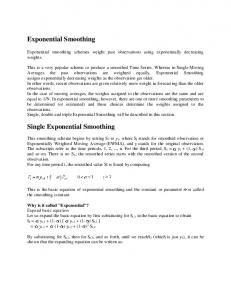
(1999) provided some insights into existing exponential smoothing theory by using a DES model within a nonparametric regression framework. Numerous studies have used DES models to forecast in a variety of fields, including environmental pollution. Collins (1976) and Chu and Lin (1994) used a DES model to forecast levels of consolidated sales and earnings as well as the relationship between expected yearly recruitment levels and the necessary target requirements in high schools in Hong Kong, respectively. In 1999, Oh et al. (1999) applied a DES model to predict ozone formation in air pollution in South Korea; and Taylor (2003) forecasted electricity demand in England and Wales by using double seasonal exponential smoothing in order to minimize the seasonal effects of electricity consumption. Elliott and Timmermann (2008) empirically applied a DES model to predict U.S. inflation and stock returns, while Taylor (2012) used it to capture the density of the number of calls arriving at call centers. On the other hand, Xie and Su (2010) applied an exponential smoothing model to develop a river water pollution predictor in China, and Gupta (2011) developed an adaptive sampling strategy by using a DES model to evaluate carbon monoxide pollution by urban road traffic. CO2 emissions in transportation are different in each state in the U.S. as a result of their geographic characteristics, levels of economic development and population growth, and transportation and environmental regulations2. Figure 1 shows CO2 emissions from the transportation sector by state in the U.S. for 2011. California and Texas emit the largest CO2 emissions, while Florida, New York, Illinois, New Jersey, Ohio, Georgia, and Pennsylvania make the second largest CO2 emissions, which are usually in areas of high development of urbanization and industrialization (U.S Energy Information Administration 2013). Figure 1: U.S. CO2 Emissions by State and the District of Columbia in 2011

64

JTRF Volume 53 No. 3, Fall 2014

Although the effect of fossil fuel energy consumption on future CO2 emissions from private vehicle use in North America was analyzed in 2008 (Poudenx 2008) and the CO2 emissions from the transportation sector in the U.S. were projected with other statistical models in 2012 (Bastani, Heywood and Hope 2012, Rentziou, Gkritza and Souleyrette 2012), their research was limited to a particular transportation industry and did not suggest future-specific CO2 emissions per state in the U.S. over time. Most importantly, their findings lacked the provision of a validity test of their forecasts. For these reasons, this study forecasts U.S. CO2 emissions by state from the overall transportation sector with the reliable validity test of pseudo out-of-sample forecasts. The objectives of this study are i) to forecast national and state-level CO2 emissions from 2012 to 2021 and ii) to review whether the decreasing trend in U.S. transportation CO2 emissions will be shown across all states during this period. From the findings, this study will be able to provide administrators and state policy planners with detailed CO2 emissions changes in the future in order to help them plan transportation CO2 emissions regulations. The second section of this study presents discussions of alternative forecasting techniques, and the third section the state and federal air pollution regulations, including GHG. The fourth and fifth sections are the methodology and the data. After the results are presented, the conclusions discuss future CO2 emissions changes in the United States. DISCUSSIONS OF ALTERNATIVE FORECASTING TECHNIQUES There exist many mathematical forecasting models today. These models include the autoregressive integrated moving average (ARIMA) technique and the seasonal autoregressive integrated moving average (S-ARIMA) technique. These methods are statistically sophisticated and mathematically complex methods that have been popular for forecasting the changes of time series in a broad number of applications (Zhai 2005). As a couple of researchers pointed out, these techniques regard past data and error terms of time series as essential information to forecast future changes. With a large amount of time series data, this technique shows quite a good accuracy of forecasting (Shumway and Stoffer 2011, Stock and Watson 2011). However, as Zhai (2005) mentioned in her research, there are a few disadvantages of ARIMA and S-ARIMA techniques compared with a DES model. First, they have many possible models due to the number of possible combinations coming from the changes of the numbers in (seasonal) autoregressive terms, (seasonal) moving average terms, and/or (seasonal) autoregressive terms. Identifying the correct model among the possible models is likely to be subjective and depends on the experience and professional knowledge of the researcher. Second, “the underlying theoretical model and structural relationships are not as distinct as a DES model.” (Zhai 2005, p.10) STATE AND FEDERAL AIR POLLUTION REGULATIONS INCLUDING GHG Of the 50 U.S. states, 32 have completed a climate change action plan to reduce their GHG emissions in their states since about 2005, which incorporates many specific policy recommendations (U.S. Environmental Protection Agency 2014C). For instance, the policy recommendations of Arkansas in 2008 included making a renewable portfolio standard, enacting a carbon tax, increasing energy efficiency, etc., and other participating states show similar policy recommendations for addressing GHG emissions (U.S. Environmental Protection Agency, 2014C). A federal regulation to reduce air pollution initially started in 1955 as the Air Pollution Control Act and was complemented over time with the Clean Air Act (1963), the Air Quality Act (1967), the Clean Air Act (1970), and the Clean Air Act Amendments (1990). Since the middle of the 2000s with the Energy Policy Act (2005), Energy Independence and Security Act (2007), and President Obama’s announcements of national policies (2009–2011 and 2014), stricter national air quality standards have been established by the U.S. Environmental Protection Agency (EPA). For more 65

CO2 Emissions

detailed information, Table 1 provides each air pollution act and its key points regarding reducing air pollution and/or GHG emissions (U.S. Environmental Protection Agency, 2014A, 2014B). Table 1: Federal Acts and Announcements and Their Key Points Federal Acts and Announcements Air Pollution Control Act (1955) Clean Air Act (1963) Air Quality Act (1967) Clean Air Act (1970) Clean Air Act Amendments (1990) Energy Policy Act (2005) Energy Independence and Security Act (2007) Obama announcements of national policies (2009–2011 and 2014)

Key points First federal-level act to prevent air pollution and provided a research fund to define scope and sources in air pollution. Establishment of a national program for preventing air pollution and started researching into techniques to reduce it. Authorized enforcement to reduce air pollution problems caused by interstate transport of pollutants. Established national air quality standards. Established a program to reduce 189 air pollutants and complemented provisions regarding the attainment of national air quality standards. Authorized to develop renewable energy or use innovative energyefficient technology for reducing air pollution, including GHG emissions. Authorized to increase energy efficiency and the production of clean renewable fuel. Presidential announcements to enhance GHG and fuel efficiency standards.

Note: Information about federal acts and announcements and their key points is from USEPA (2014A, 2014B).

METHODOLOGY Let us define: α = Smoothing weight for the level of the time series. βt = Time-varying slope. εt = Disturbances. ut = Time-varying mean. St = Smoothed state of the time series estimates ut in Eq. (1). S't = Smoothed state of the time series estimates ut in Eq. (2). S''t = Smoothed values of the S't estimates βt. Yt = Observed value at time t. = Forecast value ahead to m periods at time t. We start with a simple exponential smoothing (SES) model to derive the DES model. The model equation for the SES is: (1)

,

The smoothing equation is: (2) 66

JTRF Volume 53 No. 3, Fall 2014

The m-step prediction equation is: (3) The m-step prediction value is estimated through Eq. (1) and Eq. (2) (Elliott and Timmermann 2008, SAS 9.2 User’s Book 2013). Eq. (1) is an estimation of the time-varying mean and disturbances, while the smoothed state St that is computed after Yt is observed is updated through Eq. (2). The smoothed state is a result of the combination of its actual observation plus the first lagged smoothed state with the control of smoothed weight. Exponential smoothing does not regard the effect of each past lag equally, and rather gives more weight to recent observations; hence, the smoothing weight between 0 and 1 is adjusted for this purpose. The smoothing process is backdated from time to time 1 to determine the starting value of the smoothed state at time 0 (Chatfield and Yar 1988). The SES model cannot deal with trending data since all predictions at time t from one-stepahead to m-step-ahead are always the same as the value of in St Eq. (3). Thus, a DES model is used to reflect the effect of a trend in the data. The model equation for this is: (4)

,

The smoothing equations are: (5) (6)

The m-step prediction equation is:

(7)



The m-step prediction value is the forecast value from the DES model, which is estimated by using the same process as in the SES model, but uses another smoothed series in Eq. (5) and Eq. (6). (Elliott and Timmermann 2008, SAS 9.2 User’s Book 2013). The DES model is constructed when the SES method is twice run through the two different smoothed series in Eq. (5) and Eq. (6). The DES method can extrapolate nonseasonal patterns and trends such that the time series is smooth and has a slowly time-varying mean. DATA The data on CO2 emissions3 measured in million metric tons (MMT) from the transportation sector in the 50 states and the District of Columbia through fossil fuel combustion were obtained from the EPA for 1990‒2011 (U.S. Environmental Protection Agency 2013). However, according to the central limit theorem, only 22 observations in a state may not be large enough to make the assumption that our sample data are well approximated by a normal distribution. To confirm this statistically, the normality of every state’s CO2 emissions data was tested by using an Anderson–Darling test, and the null hypothesis of no normality was not rejected, even at the 10% significance level. Nevertheless, motor gasoline consumption data,4 which are strongly correlated with CO2 emissions from the transportation sector, were available for 1960‒2011 from the State Energy Data System in the U.S. Energy Information Administration (USEIA) (U.S Energy Information Administration 2013). Thus, following some calculation processes, 29 new observations in each state from 1960 to 1989 were added for the state-level CO2 emissions. First, we calculated the ratio of CO2 emissions and motor gasoline consumption from 1990 to 2011 in a state. Second, we 67

CO2 Emissions

summed the 22 calculated ratios and divided it by 22 to find the average annual CO2 emissions per unit of motor gasoline consumption (the value of 22 was from the difference between 1990 and 2011). Third, motor gasoline consumption from 1960 to 1989 in a state was multiplied by the calculation result from step 2. Finally, the CO2 emissions for the transportation sector from 1960 to 1989 by state were calculated through the third process. To check that the new dataset from 1960 to 2011 was normally distributed, an Anderson–Darling test in each state was again performed, and the non-normality assumption was statistically rejected at the 5% significance level. Table 2 shows the CO2 emissions from the transportation sector in the 50 states, the District of Columbia, and the U.S. for 1960‒2011. Total U.S. CO2 emissions increased until 2007, but decreased thereafter. Most states showed a similar trend, but 14 states have recently increased their CO2 emissions: Alabama, Alaska, Hawaii, Idaho, Iowa, Louisiana, Nebraska, New Jersey, North Dakota, Ohio, Oklahoma, Tennessee, Texas, and Utah. EMPIRICAL RESULTS Before discussing the empirical results, this study’s discussion is built around an assumption based on a technical report from the U.S. Energy Information Administration (2014). We assumed that motor gasoline consumption in the transportation sector will decrease in the next 10 years even though the U.S. economic recovery occurs, since a decrease in vehicle mileage from passenger cars, which is a possible cause of the recent decrease in CO2 emissions in the U.S. transportation sector, is expected to be maintained. As discussed in the methodology section, an SES model was not appropriate with the trending data of CO2 emissions in the U.S. transportation sector, since it only gives reliable forecasts when a time series fluctuates about a base level. For this reason, a DES model that yields good forecasts with trending data was performed to forecast CO2 emissions in the U.S. transportation sector. Pseudo out-of-sample forecasts5 were estimated to test the out-of-sample performances of the DES models in each state and the U.S. The models were fitted with the CO2 emissions data from 1960 to 2005, and then the forecasted CO2 emissions from 2006 to 2011 were compared with the actual observations during the same period, which were 10% of the sample size to verify forecasting accuracy. Table 3 provides the actual observations and 95% forecast confidence intervals for 2006‒2011. The overall forecasting accuracies by the DES models in the 47 states and the U.S. are high; the actual observations of CO2 emissions in 20 states are within the 95% forecast confidence intervals, which means that in 95% of all samples, they would contain the actual CO2 emissions; 27 states and the U.S. only have one or two actual observations of CO2 emissions among six of the 95% forecast confidence interval(s). On the other hand, Alaska, Idaho, North Carolina, and North Dakota show poor forecasting accuracies since three or four actual observations of CO2 emissions are not within the 95% forecast confidence intervals for 2006‒2011. Next, the DES models in every state, the District of Columbia, and the U.S. were regressed with the transportation CO2 emissions data from 1960 to 2011 by using the statistical package program SAS 9.3. The regression results in Table 4 show the parameter estimates for smoothed level, smoothed trend, smoothing weight, root mean square error (RMSE), and goodness of fit (R2). Columns 1, 2, and 3 start with the information on smoothed level, smoothed trend, and smoothing weight, with the three concepts explained as follows: if a smoothed level is 1869 and a smoothed trend is -19.8, then the forecast value in the first forecast year has a value of 1849 (=1869-19.8). In the second forecast year, the forecast value is 1829 (=1849-19.8), and so on. A smoothing weight between 0 and 1 is adjusted to give more weight to recent observations. All the models in the 50 states, the District of Columbia, and the U.S. in Table 4 have statistically significant smoothing weights at 1%, and the overall model fits run from 0.8 to 0.98, meaning that the DES models used show high model fits for 1960–2021. On the other hand, the RMSE increases 68

JTRF Volume 53 No. 3, Fall 2014

when the CO2 emissions in a state increase, and thus California, Florida, and Texas show high RMSEs relative to the other states. To make the estimation efficient and proper, a Ljung–Box chi-square test for error autocorrelation and a Dickey–Fuller test for stationarity were performed. In the DES models of each state and the U.S., the Ljung–Box chi-square tests showed that the autocorrelations of lags 1 and 2 in the prediction error are zero at the 1% significance level, while the Dickey–Fuller tests showed that a stationary time series is likely at the 1% significance level. The lagged variables in the DES models were assumed to be exogenous since the error terms were not serially correlated (Gujarati and Porter 2009). In Table 4, the District of Columbia, Idaho, Iowa, Kansas, Nebraska, North Dakota, Oklahoma, South Dakota, Tennessee, and Utah are projected to increase CO2 emissions from the transportation sector for 2012‒2021 since their smoothed trends are greater than 0; however, owing to the possible poor forecasting accuracy of North Dakota in the pseudo out-of-sample forecast procedure, the findings for this state need to be carefully interpreted. On the other hand, 41 states are projected to show a decrease in CO2 emissions because of the negative smoothed trends in Table 4. The levels of decreasing emissions will be different in each state, with California showing the largest CO2emissions decrease due to the largest negative smoothed trend value of -5.31. Table 5 shows the forecast values of CO2 emissions from the transportation sector in the 50 states, the District of Columbia, and the U.S. for 2012‒2021. The summation of CO2emissions in all states is well matched to the forecast of U.S. CO2 emissions. In California, CO2 emissions from the transportation sector will significantly decrease by as much as one quarter of its 2011 CO2 emissions by 2021, while Texas and Florida, which emitted the second and third highest CO2 emissions in 2011, will gradually decrease their CO2 emissions, too. In contrast, the 10 states in Table 4 projected to increase CO2 emissions will increase their CO2 emissions for 2012‒2021, but their proportion of total CO2 emissions will only range from 9% to 11% during this period; hence, the overall decreasing CO2 emissions trend in the U.S. will remain. The findings for these 10 states might be a result of factors such as sudden population increases, less strict air pollution regulations in the transportation sector, and/or local economic growth through oil booms, agriculture production increases, or industrial development.

69

CO2 Emissions

Table 2: CO2 Emissions from the Transportation Sector by State, the District of Columbia, and the U.S. from 1960 to 2011 (Unit: MMT) State/Year

1960

1970

1980

1990

2000

2007

2009

2011

Alabama

13.6

20.7

24.9

28.1

33.6

36.2

32.7

33.6

Arizona

6.7

11.9

17.0

22.8

32.5

38.0

33.1

31.7

Arkansas

8.5

13.3

15.9

16.2

21.0

21.2

20.4

20.1

Alaska

3.6

5.3

7.7

12.1

15.7

18.0

13.7

14.3

California

82.9

131.6

156.2

202.8

215.8

238.1

217.5

207.7

Colorado

8.6

14.2

19.0

19.2

25.7

31.5

29.4

28.9

Connecticut

9.0

13.3

14.1

14.7

16.2

17.7

16.4

15.8

Delaware

2.1

3.2

3.4

4.5

5.1

5.2

4.8

4.2

District of Columbia

2.2

2.6

1.8

1.8

1.8

1.2

1.1

1.2

Florida

23.4

41.3

59.6

81.4

100.6

115.7

99.4

105.6

Georgia

17.6

30.6

37.2

48.7

61.5

67.1

65.4

65.0

Hawaii

3.5

5.9

7.6

11.1

9.0

14.1

9.5

10.2

Idaho

3.5

5.3

6.1

6.4

8.8

9.6

8.7

9.1

Illinois

39.3

55.6

57.8

54.4

67.1

73.8

68.4

66.9

Indiana

25.2

35.0

36.8

40.9

46.6

45.5

40.9

42.9

Iowa

12.9

16.5

17.8

16.3

18.8

22.3

21.1

21.8

Kansas

12.1

16.5

17.9

19.3

18.8

19.6

19.8

19.1

Kentucky

13.3

21.2

25.3

26.4

31.5

35.0

32.7

32.6

Louisiana

23.1

36.3

49.9

48.9

61.0

50.8

47.2

50.2

Maine

4.4

5.8

6.2

8.3

8.6

9.1

8.6

8.4

Maryland

10.7

18.1

21.5

23.6

28.6

31.7

31.8

29.3

Massachusetts

17.1

24.3

25.2

28.9

32.1

33.6

30.8

30.9

Michigan

30.2

45.3

46.2

47.9

57.3

55.4

50.0

48.7

Minnesota

15.8

22.6

25.0

23.8

35.0

36.5

32.3

32.3

Mississippi

10.6

16.6

18.5

20.2

25.2

26.7

25.1

24.6

Missouri

21.2

29.9

32.0

33.8

39.5

42.9

39.7

39.4

Montana

4.0

5.7

6.5

5.9

7.5

9.0

8.0

8.2

Nebraska

6.5

8.6

9.2

10.5

12.2

12.6

12.5

14.2

Nevada

2.2

4.5

7.0

9.4

14.5

18.3

14.8

13.4

New Hampshire

2.2

3.6

4.1

5.2

7.3

7.5

7.2

7.1

New Jersey

33.1

45.2

50.1

57.1

65.0

72.6

62.3

66.0

New Mexico

6.5

9.1

11.8

14.9

15.3

15.6

14.0

14.1

New York

47.1

65.0

64.2

64.1

67.2

74.6

72.4

67.0

North Carolina

17.4

27.7

32.7

38.4

50.0

54.9

49.0

47.8

North Dakota

3.4

4.5

5.4

4.6

5.6

7.1

6.0

8.1

Ohio

41.3

57.8

61.1

56.1

68.9

72.9

64.6

65.2

Oklahoma

14.7

22.1

27.1

23.9

30.3

32.5

31.1

32.0

Oregon

9.7

15.4

19.1

20.0

22.7

24.5

22.9

21.2

Pennsylvania

44.1

56.4

61.6

59.5

70.6

72.2

66.4

64.5

70

JTRF Volume 53 No. 3, Fall 2014

Table 2 (continued) State/Year

1960

1970

1980

1990

2000

2007

2009

2011

Rhode Island

2.8

3.8

4.0

4.1

4.7

4.4

4.3

4.0

South Carolina

8.8

14.4

18.0

22.0

27.1

32.2

31.3

30.9

South Dakota

3.5

4.6

4.9

4.7

5.8

6.4

6.3

6.6

Tennessee

15.7

24.5

32.4

32.8

41.6

46.3

41.6

43.1

Texas

64.2

102.3

130.2

152.5

182.9

205.1

190.2

195.5

Utah

4.8

7.9

10.2

10.6

15.7

18.5

16.4

17.5

Vermont

1.5

2.4

2.6

3.0

3.7

3.9

3.6

3.4

Virginia

16.9

26.9

32.9

41.5

48.6

57.2

50.9

48.3

Washington

15.8

25.3

30.1

41.0

44.8

47.9

42.2

41.2

West Virginia

6.9

9.5

11.7

10.4

12.7

12.5

11.4

11.2

Wisconsin

15.3

21.9

24.4

24.3

29.8

31.1

29.5

29.2

Wyoming

4.0

5.3

8.0

5.8

7.6

8.9

8.3

7.8

U.S. Total

814

1217

1420

1585

1880

2045

1868

1862

Note: The CO2 emissions for the transportation sector from 1960 to 1989 by state and the District of Columbia were calculated using motor gasoline consumption data from 1960 to 1989 in USEIA (2013); the CO2 emissions from 1990 to 2011 were obtained from USEPA (2013).

71

CO2 Emissions

Table 3: Pseudo Out-of-Sample Forecasts of CO2 Emissions (MMT) from the Transportation Sector to Evaluate the DES Models’ Performances by State, the District of Columbia, and the U.S. from 2006 to 2011 State/Year

2006

2007

2008

2009

2010

2011

Alabama

35.5 (33.7, 37.6)

36.1 (34.2, 38.1)

33.5† (34.7, 38.7)

32.6 (31.8, 35.7)

33.7 (30.1, 34.0)

33.5 (31.1, 35.1)

Arizona

38.2 (36.7, 39.0)

37.9† (38.0, 40.4)

35.0† (37.3, 39.7)

33.1 (33.2, 35.6)

32.0 (30.4, 32.8)

31.7 (29.3, 31.7)

Arkansas

20.6 (19.1, 22.4)

21.1 (19.1, 22.4)

20.5 (19.6, 22.8)

20.3 (19.0, 22.3)

20.4 (18.7, 21.9)

20.1 (18.7, 21.9)

Alaska

19.1 (17.9, 21.6)

18.0† (18.2, 22.0)

15.4† (17.3, 21.1)

13.6† (14.7, 18.5)

15.0 (12.1, 15.9)

14.2 (12.2, 16.0)

California

234 (221, 245)

238 (226, 250)

222† (230, 254)

217 (212, 237)

215 (202, 226)

207 (198, 223)

Colorado

30.7 (29.2, 32.3)

31.5 (30.1, 33.2)

30.1† (30.8, 34.0)

29.3 (29.3, 32.5)

29.8 (27.9, 31.1)

28.8 (28.1, 31.2)

Connecticut

17.6† (18.1, 20.0)

17.6 (17.0, 18.9)

16.7 (16.6, 18.6)

16.4 (15.7, 17.6)

16.1 (15.1, 17.0)

15.8 (14.7, 15.7)

5.1 (4.7, 5.6)

5.2 (4.8, 5.6)

5.0 (4.9, 5.7)

4.8 (4.6, 5.4)

4.4 (4.4, 5.2)

4.2 (4.0, 4.8)

District of Columbia

1.23 (1.15, 1.56)

1.22 (0.94, 1.35)

1.07 (0.90, 1.32)

1.12 (0.77, 1.18)

1.10 (0.82, 1.24)

1.22 (0.83, 1.25)

Florida

116 (111, 124)

115 (113, 127)

105† (111, 125)

99 (99, 113)

105† (89, 103)

105 (95, 109)

Georgia

68.3 (68.2, 74.4)

67.0 (66.8, 73.0)

61.2† (64.4, 70.7)

65.4† (56.7, 62.9)

66.7 (61.2, 67.4)

65.0 (63.9, 70.1)

Hawaii

13.0 (12.5, 14.6)

14.0 (12.5, 14.6)

9.71† (13.6, 15.7)

9.44 (7.93, 10.0)

9.65† (7.14, 9.28)

10.23† (7.81, 9.95)

Idaho

9.30 (8.17, 9.31)

9.63 (8.92, 10.06)

8.78† (9.36, 10.51)

8.68 (8.22, 9.36)

9.47† (7.94, 9.08)

9.13 (8.97, 10.12)

Illinois

73.3† (75.3, 87.9)

73.7 (68.9, 81.5)

69.8 (67.9, 80.5)

68.3 (62.1, 74.7)

67.6 (60.2, 72.8)

66.8 (60.0, 72.6)

Indiana

46.4 (42.2, 49.0)

45.5 (43.0, 49.9)

42.3† (42.4, 24.2)

40.8 (39.0, 45.8)

42.9 (36.7, 43.5)

42.9 (38.2, 45.1)

Iowa

21.8 (20.5, 23.4)

22.3 (21.0, 23.9)

21.5 (21.4, 24.3)

21.1 (20.1, 23.0)

21.5 (19.4, 22.2)

21.7 (20.0, 22.9)

Kansas

19.0 (16.5, 19.8)

19.5 (17.1, 20.4)

19.0 (17.8, 21.1)

19.7 (17.6, 20.9)

19.6 (18.2, 21.4)

19.0 (18.1, 21.4)

Kentucky

33.4 (32.1, 36.3)

34.9 (31.8, 36.0)

32.1† (33.1, 37.2)

32.6 (30.7, 34.8)

33.2 (30.4, 34.5)

32.6 (30.9, 35.0)

Louisiana

55.0 (46.6, 54.8)

50.8 (49.5, 57.7)

47.9 (46.8, 55.0)

47.2 (43.4, 51.6)

50.1† (41.8, 50.0)

50.2 (44.3, 52.5)

Maine

9.41 (8,67, 10.3)

9.06 (8.80, 10.4)

8.20† (8.49, 10.1)

8.57 (7.59, 9.25)

8.51 (7.59, 9.52)

8.38 (7.56, 9.22)

Maryland

42.2 (39.0, 45.1)

42.8 (39.6, 45.6)

40.3 (40.3, 46.4)

39.6 (36.4, 42.5)

40.1 (35.6, 41.6)

39.3 (36.8, 42.8)

Massachusetts

33.0† (33.3, 36.3)

33.5 (31.6, 34.5)

33.4 (32.1, 35.1)

30.7† (32.0, 34.9)

30.8 (28.4, 31.3)

30.9 (28.4, 31.4)

Michigan

55.7 (52.1, 59.1)

55.3 (52.0, 59.0)

51.3† (51.6, 58.6)

49.9 (45.6, 52.6)

49.8 (44.5, 51.4)

48.6 (45.3, 52.3)

Minnesota

36.1 (34.9, 39.4)

36.5 (34.3, 38.8)

34.6 (34.4, 39.0)

32.2 (32.2, 36.7)

32.7 (29.1, 33.6)

32.3 (29.5, 34.0)

Delaware

72

JTRF Volume 53 No. 3, Fall 2014

Table 3 (continued)

State/Year

2006

2007

2008

2009

2010

2011

Mississippi

26.8 (23.8, 26.9)

26.6 (25.4, 28.5)

25.6 (25.4, 28.5)

25.0 (24.1, 27.2)

25.2 (23.2, 26.2)

24.6 (23.4, 26.5)

Missouri

42.2 (39.0, 45.1)

42.8 (39.6, 45.6)

40.3 (40.3, 46.4)

39.6 (36.4, 42.5)

40.1 (35.6, 41.6)

39.3 (36.8, 42.8)

Montana

8.5 (7.5, 9.0)

9.0 (7.9, 9.4)

8.3† (8.4, 9.9)

7.9† (8.0, 9.5)

8.1 (7.5, 9.0)

8.2 (7.4, 8.9)

Nebraska

12.4 (11.3, 13.4)

12.6 (11.5, 13.6)

12.3 (11.7, 13.8)

12.5 (11.2, 13.3)

14.6 (11.4, 13.6)

14.1 (14.8, 17.0)

Nevada

18.0 (16.8, 18.0)

18.2 (18.1, 19.3)

16.3† (18.4, 19.6)

14.8† (15.9, 17.1)

13.9 (13.6, 14.8)

13.3 (12.4, 13.6)

7.2 (6.8, 7.8)

7.4 (6.6, 7.6)

7.2 (6.9, 7.8)

7.2 (6.7, 7.7)

7.2 (6.6, 7.6)

7.0 (6.6, 7.6)

New Jersey

68.8 (65.7, 73.4)

72.6 (66.5, 74.2)

73.5 (69.9, 77.6)

62.2† (71.5, 79.2)

63.7 (61.1, 68.8)

65.9 (58.9, 66.6)

New Mexico

16.0 (14.0, 16.9)

15.5 (14.5, 17.4)

14.2† (14.3, 17.1)

14.0 (13.0, 15.8)

13.6 (12.3, 15.2)

14.1 (11.9, 14.7)

New York

74.8 (69.4, 82.4)

74.6 (69.6, 82.7)

74.3 (69.2, 82.2)

72.3 (68.6, 81.6)

72.3 (66.5, 79.5)

66.9 (65.7, 78.7)

North Carolina

53.1 (53.0, 56.9)

54.9 (51.2, 55.1)

53.4† (54.1, 58.1)

48.9† (50.8, 54.8)

49.2† (43.7, 47.6)

47.7 (46.2, 50.1)

North Dakota

6.2 (5.8, 7.0)

7.1† (5.7, 6.9)

6.3† (6.4, 7.6)

6.0† (6.1, 7.2)

6.9† (5.6, 6.8)

8.0† (6.2, 7.3)

Ohio

72.1 (67.6, 75.7)

72.9 (68.6, 76.6)

69.0† (69.5, 77.6)

64.5 (63.2, 71.2)

65.9† (57.0, 65.0)

65.2 (60.9, 69.0)

Oklahoma

31.7 (28.0, 33.0)

32.5 (29.2, 34.2)

32.3 (30.3, 35.3)

31.0 (30.3, 35.3)

32.2 (28.9, 33.9)

31.9 (29.6, 34.6)

Oregon

23.9 (22.4, 25.2)

24.5 (23.0, 25.8)

22.7† (23.7, 26.4)

22.9 (21.1, 23.8)

22.1 (21.1, 23.9)

21.2 (20.3, 23.0)

Pennsylvania

72.4 (70.1, 78.2)

72.2 (68.3, 76.4)

67.4† (67.9, 76.0)

66.4 (59.5, 67.6)

66.0† (60.7, 68.8)

64.4 (61.4, 69.5)

Rhode Island

4.4 (4.0, 4.5)

4.3 (4.1, 4.6)

4.1 (4.1, 4.6)

4.2 (3.8, 4.3)

4.2 (3.9, 4.4)

4.0 (3.9, 4.4)

South Carolina

32.0 (30.2, 33.7)

32.2 (31.1, 34.6)

30.6† (31.3,34.8)

31.2 (29.7, 33.2)

31.2 (29.7, 33.2)

30.8 (29.6, 33.1)

South Dakota

6.1 (5.6, 6.6)

6.4 (5.6, 6.7)

6.0 (5.9, 7.0)

6.2 (5.5, 6.6)

6.5 (5.7, 6.8)

6.5 (6.1, 7.1)

Tennessee

45.8 (43.8, 48.4)

46.2 (44.0, 48.6)

42.9† (44.3, 48.9)

41.5 (39.9, 44.5)

43.1† (37.9, 42.5)

43.1 (40.1, 44.8)

Texas

202 (186, 206)

205 (194, 214)

197 (198, 218)

190† (190, 210)

194 (179, 199)

195 (182, 201)

Utah

18.5† (16.2, 17.9)

18.5 (18.3, 20.0)

17.0† (18.3, 20.0)

16.4 (16.2, 17.9)

16.3 (15.1, 16.8)

17.4 (15.1, 16.8)

Vermont

3.8 (3.7, 4.1)

3.8 (3.7, 4.1)

3.5 (3.6, 4.0)

3.6 (3.2, 3.6)

3.5 (3.3, 3.7)

3.4 (3.2, 3.6)

Virginia

56.9 (55.4, 60.1)

57.2 (56.3, 61.0)

52.7 (56.0, 60.7)

50.8 (49.7, 54.3)

50.4 (46.7, 51.4)

48.3 (46.6, 51.2)

Washington

44.8 (40.3, 46.7)

47.8 (41.8, 48.1)

42.9 (45.1, 51.5)

42.1 (41.0, 47.3)

41.2 (38.9, 45.2)

41.1 (37.5, 43.8)

New Hampshire

73

CO2 Emissions

Table 3 (continued) State/Year

2006

2007

2008

2009

2010

2011

West Virginia

12.5 (11.6, 13.6)

12.4 (11.6, 13.6)

11.0† (11.5, 13.5)

11.3 (9.8, 11.9)

11.6 (9.9, 12.0)

11.2 (10.4, 12.5)

Wisconsin

30.8 (28.9, 31.9)

31.1 (29.5, 32.6)

30.1 (29.8, 32.9)

29.5 (28.3, 31.3)

30.3 (27.4, 30.4)

29.1 (28.8, 31.9)

Wyoming

8.6 (7.5, 9.3)

8.8 (7.8, 9.6)

8.6 (8.1, 9.9)

8.3 (7.9, 9.7)

8.4 (7.5, 9.3)

7.7 (7.5, 0.3)

U.S. Total

2028 (1962, 2106)

2045 (1990, 2133)

1929† (1998, 2141)

1867 (1807, 1950)

1891† (1731, 1874)

1862 (1801, 1944)

Note: † indicates that actual CO2 emissions are not within the 95% forecast confidence interval. Actual CO2 emissions are out of the parentheses, and 95% forecast confidence intervals are in the parentheses.

CONCLUSIONS The increase in CO2 emissions in the world has adversely affected sustainable development for human life and the Earth’s ecosystems, resulting in global warming and climate change; therefore, the recent decrease in CO2 emissions from the U.S. transportation sector and its long-term decreasing trend found in this study are meaningful for the world’s efforts to reduce CO2 emissions. This study found that the decreases in CO2 emissions in most states are not temporary, but rather will continuously occur for the next decade. By 2021, the U.S. is projected to emit CO2 of 1664 MMT from the transportation sector, a reduction of 198 MMT compared with 2011. This reduced amount in 2021 will account for almost all the CO2 emissions from California in 2011, which emitted the most CO2 emissions in the nation. A major finding from the empirical results is that while CO2 emissions by most of the U.S. states for the next 10 years will show a downward pattern, 10 states are projected to show an increasing tendency of transportation CO2 emissions. One possible hypothesis to explain this difference across states is probably related to whether a state has a GHG emissions reduction plan in place or not. Looking at these 10 states, eight of them have not actually completed any climate change action plan within their boundaries, compared with most of the other states trying to address GHG emissions. This could imply much more importance needs to be placed on environmental policies for CO2 emissions reduction in the transportation sector, not only at national but at state level, too. One caveat, nevertheless, is that from this finding, the policymakers should really aim at those areas where the policy might be warranted, i.e., by the Lucas Critique,6 if a policy changes, the outcomes of sample forecasts will be wrong. This study has a limitation based on the data used. The CO2 emissions data from 1960 to 1989 for each state and the U.S. were estimated from motor gasoline consumption data to find the best possible approximation; if original data during the period were available from the EPA, we could have estimated more accurate results for our CO2 emissions forecasts from the U.S. transportation sector.

74

JTRF Volume 53 No. 3, Fall 2014

Table 4: Parameter Estimates, a Measure of Accuracy, and Goodness of Fit for Projections of CO2 Emissions by State, the District of Columbia, and the U.S. for 2012–2021 State

Smoothed Level

Smoothed Trend

Smoothing Weight

RMSE

R2

Alabama

33.59

-0.12

0.56 ***

1.06

0.97

Arizona

31.80

-0.63

0.83 ***

0.77

0.99

Arkansas

20.28

-0.13

0.51 ***

0.78

0.95

Alaska

14.64

-0.50

0.53 ***

1.13

0.93

California

211.74

-5.31

0.59 ***

6.43

0.97

Colorado

29.27

-0.37

0.57 ***

0.84

0.98

Connecticut

16.05

-0.35

0.58 ***

0.51

0.94

Delaware

4.46

-0.21

0.51 ***

0.20

0.94

District of Columbia

1.17

0.02

0.57 ***

0.10

0.94

Florida

105.33

-0.33

0.56 ***

3.47

0.98

Georgia

65.41

-0.04

0.52 ***

1.99

0.98

Hawaii

10.10

-0.19

0.55 ***

0.90

0.87

Idaho

9.15

0.04

0.51 ***

0.34

0.96

Illinois

67.44

-1.06

0.62 ***

3.25

0.85

Indiana

42.84

-0.22

0.48 ***

1.72

0.91

Iowa

21.69

0.16

0.71 ***

0.71

0.91

Kansas

19.31

0.004

0.44 ***

0.80

0.84

Kentucky

32.88

-0.12

0.47 ***

1.04

0.96

Louisiana

49.85

-0.20

0.43 ***

2.20

0.95

Maine

8.50

-0.08

0.43 ***

0.41

0.91

Maryland

29.78

-0.87

0.70 ***

1.50

0.98

Massachusetts

31.04

-0.38

0.61 ***

0.85

0.96

Michigan

49.05

-1.00

0.73 ***

1.76

0.94

Minnesota

32.63

-0.59

0.58 ***

1.13

0.96

Mississippi

24.97

-0.32

0.55 ***

0.78

0.97

Missouri

39.60

-0.44

0.70 ***

1.50

0.94

Montana

8.23

-0.004

0.41***

0.39

0.89

Nebraska

14.05

0.44

0.63 ***

0.62

0.91

Nevada

13.48

-0.69

0.87 ***

0.49

0.98 0.98

New Hampshire

7.15

-0.07

0.59 ***

0.23

New Jersey

65.91

-0.57

0.42 ***

2.63

0.93

New Mexico

14.13

-0.21

0.45 ***

0.71

0.93

New York

70.25

-1.59

0.48 ***

3.21

0.80 0.98

North Carolina

48.29

-1.25

0.71 ***

1.26

North Dakota

7.10

0.26

0.36 ***

0.38

0.84

Ohio

65.38

-0.55

0.77 ***

2.03

0.94

Oklahoma

31.91

0.08

0.47 ***

1.23

0.93

Oregon

21.61

-0.72

0.66 ***

0.72

0.96

Pennsylvania

64.78

-1.30

0.83 ***

2.08

0.93 75

CO2 Emissions

Table 4 (continued) State

Smoothed Level

Smoothed Trend

Smoothing Weight

RMSE

R2

Rhode Island

4.11

-0.08

0.56 ***

0.12

0.93

South Carolina

31.04

-0.07

0.49 ***

0.90

0.98

South Dakota

6.49

0.09

0.54 ***

0.26

0.89

Tennessee

43.03

0.005

0.64 ***

1.28

0.97

Texas

195.03

-0.34

0.53 ***

5.22

0.98

Utah

17.13

0.22

0.62 ***

0.59

0.97

Vermont

3.47

-0.08

0.61 ***

0.11

0.97

Virginia

48.99

-1.64

0.73 ***

1.38

0.98

Washington

41.78

-0.67

0.48 ***

1.76

0.96

West Virginia

11.43

-0.14

0.50 ***

0.54

0.89

Wisconsin

29.47

-0.43

0.68 ***

0.78

0.97

Wyoming

8.14

-0.17

0.49 ***

0.44

0.90

U.S. Total

1869

-19.81

0.75 ***

41.10

0.98

Note: *** indicate significance at the 1% level. The smoothed level and trend are not related to the hypothesis tests. The smoothed level and trend and smoothing weight use a unit of MMT CO2.

76

JTRF Volume 53 No. 3, Fall 2014

Table 5: Forecasted Values of CO2 Emissions from the Transportation Sector by State, the District of Columbia, and the U.S. from 2012 to 2021 (Unit: MMT) State/Year

2012

2013

2014

2015

2016

2017

2018

2019

2020

2021

Alabama

33.4

33.2

33.1

33.0

32.9

32.8

32.6

32.5

32.4

32.3

Arizona

31.0

30.4

29.8

29.1

28.5

27.9

27.2

26.6

26.0

25.3

Arkansas

20.0

19.9

19.8

19.6

19.5

19.4

19.2

19.1

18.9

18.8

Alaska

13.7

13.2

12.7

12.2

11.7

11.2

10.7

10.2

9.7

9.2

California

202.8

197.5

192.2

186.9

181.5

176.2

170.9

165.6

160.3

155.0

Colorado

28.6

28.2

27.9

27.5

27.1

26.7

26.4

26.0

25.6

25.2

Connecticut

15.4

15.1

14.7

14.4

14.0

13.7

13.3

12.9

12.6

12.2

Delaware

4.0

3.8

3.6

3.4

3.2

3.0

2.8

2.6

2.3

2.1

District of Columbia

1.2

1.2

1.3

1.3

1.3

1.3

1.3

1.4

1.4

1.4

Florida

104.7

104.4

104.0

103.7

103.4

103.0

102.7

102.4

102.1

101.7

Georgia

65.3

65.2

65.2

65.2

65.1

65.1

65.0

65.0

64.9

64.9

Hawaii

9.7

9.5

9.3

9.1

8.9

8.8

8.6

8.4

8.2

8.0

Idaho

9.2

9.2

9.3

9.3

9.4

9.4

9.5

9.5

9.5

9.6

Illinois

65.7

64.6

63.6

62.5

61.4

60.4

59.3

58.3

57.2

56.1

Indiana

42.3

42.1

41.9

41.7

41.5

41.2

41.0

40.8

40.6

40.3

Iowa

21.9

22.0

22.2

22.4

22.5

22.7

22.9

23.0

23.2

23.4

Kansas

19.3

19.3

19.3

19.3

19.3

19.3

19.3

19.3

19.3

19.3

Kentucky

32.6

32.4

32.3

32.2

32.0

31.9

31.8

31.7

31.5

31.4

Louisiana

49.3

49.1

48.9

48.7

48.5

48.3

48.1

47.9

47.7

47.5

Maine

8.3

8.2

8.1

8.0

7.9

7.8

7.7

7.6

7.5

7.4

Maryland

28.4

27.5

26.6

25.7

24.9

24.0

23.1

22.2

21.4

20.5

Massachusetts

30.4

30.0

29.6

29.2

28.8

28.4

28.1

27.7

27.3

26.9

Michigan

47.6

46.6

45.6

44.6

43.6

42.6

41.6

40.6

39.6

38.6

Minnesota

31.6

31.0

30.4

29.8

29.2

28.6

28.0

27.4

26.8

26.2

Mississippi

24.3

24.0

23.7

23.4

23.1

22.7

22.4

22.1

21.8

21.4

Missouri

38.9

38.5

38.0

37.6

37.1

36.7

36.3

35.8

35.4

34.9

Montana

8.2

8.2

8.2

8.2

8.2

8.1

8.1

8.1

8.1

8.1

Nebraska

14.7

15.1

15.6

16.0

16.5

16.9

17.3

17.8

18.2

18.7

Nevada

12.6

11.9

11.3

10.6

9.9

9.2

8.5

7.8

7.1

6.4

New Hampshire

7.0

6.9

6.8

6.8

6.7

6.6

6.5

6.5

6.4

6.3

New Jersey

64.5

63.9

63.3

62.8

62.2

61.6

61.0

60.5

59.9

59.3

New Mexico

13.6

13.4

13.2

13.0

12.8

12.6

12.4

12.1

11.9

11.7

New York

66.7

65.1

63.5

61.9

60.3

58.7

57.1

55.5

53.9

52.3

North Carolina

46.5

45.2

44.0

42.7

41.4

40.2

38.9

37.7

36.4

35.2

North Dakota

7.8

8.0

8.3

8.6

8.8

9.1

9.4

9.6

9.9

10.1

Ohio

64.6

64.1

63.5

63.0

62.4

61.8

61.3

60.7

60.2

59.6

Oklahoma

32.0

32.1

32.2

32.3

32.4

32.5

32.6

32.7

32.8

32.9

Oregon

20.5

19.8

19.0

18.3

17.6

16.9

16.2

15.4

14.7

14.0

Pennsylvania

63.2

61.9

60.6

59.3

58.0

56.7

55.4

54.1

52.8

51.5

Rhode Island

3.9

3.8

3.7

3.6

3.6

3.5

3.4

3.3

3.2

3.1

77

CO2 Emissions

Table 5 (continued) State/Year

2012

2013

2014

2015

2016

2017

2018

2019

2020

2021

South Carolina

30.8

30.8

30.7

30.6

30.5

30.5

30.4

30.3

30.2

30.2

South Dakota

6.6

6.7

6.8

6.9

7.0

7.1

7.2

7.3

7.4

7.5

Tennessee

43.0

43.0

43.0

43.0

43.0

43.0

43.0

43.0

43.0

43.0

Texas

194.3

194.0

193.6

193.3

193.0

192.6

192.3

191.9

191.6

191.2

Utah

17.4

17.7

17.9

18.1

18.4

18.6

18.8

19.0

19.3

19.5

Vermont

3.3

3.2

3.1

3.0

2.9

2.8

2.8

2.7

2.6

2.5

Virginia

46.7

45.0

43.4

41.7

40.1

38.5

36.8

35.2

33.5

31.9

Washington

40.3

39.7

39.0

38.3

37.6

37.0

36.3

35.6

35.0

34.3

West Virginia

11.1

10.9

10.8

10.6

10.5

10.3

10.2

10.0

9.9

9.7

Wisconsin

28.8

28.4

27.9

27.5

27.0

26.6

26.2

25.7

25.3

24.9

Wyoming

7.7

7.6

7.4

7.2

7.0

6.9

6.7

6.5

6.3

6.1

U.S. Total

1843

1823

1803

1783

1763

1744

1724

1704

1684

1664

Endnotes 1. The EPA defines light-duty vehicles (i.e., passenger cars) as carrying a maximum Gross Vehicle Weight Rating of less than 8500 lbs (The U.S. Energy Information Administration 2014). 2. These variables are embodied in the trend of the change in CO2 emissions. The change of CO2 emissions in the transportation sector are highly related to these factors, so if we use those variables as explanatory variables with CO2 emissions variable in a forecasting model, then it could result in multicollinearity. Also, DES models only use one variable that we are trying to forecast. For example, suppose we are interested in forecasting CO2 emissions in the transportation sector. The dependent variable and independent variables using the DES model will be calculated through the mathematical formula of the DES model from only the one variable. 3. CO2 emissions per kWh in electricity from coal-fired thermal power stations are reported higher than in CO2 emissions per kWh from various other fuels (Hutton 2013). 4. CO2 emissions are generated by both gasoline consumption and diesel consumption data. Due to the non-availability of diesel consumption data to the public, this study could only use gasoline consumption data. 5. Pseudo out-of-sample forecasting is generally used to test the real-time accuracy of a forecasting model. The mechanism is as follows: Select a date close to the end of the sample, estimate a forecasting model with data up to that date, utilize the estimated forecasting model to make a forecast after the date, and then compare the forecasted values corresponding to the original data (Stock and Watson 2011). 6. The Lucas Critique derived from his work on macroeconomic policymaking implies that evaluation of the effects of economic policy based on the historical data might not be appropriate (Lucas 1976).

78

JTRF Volume 53 No. 3, Fall 2014

Acknowledgements This research was part of Jaesung Choi’s dissertation and was funded by the Mountain-Plains Consortium, the Region 8 University Transportation Center at North Dakota State University. References Bastani, Parisa, John B. Heywood, and Chris Hope. “The Effect of Uncertainty on US Transport Related GHG Emissions and Fuel Consumption Out to 2050.” Transportation Research Part A, (2012): 517-548. Brown, Robert G. “Exponential Smoothing For Predicting Demand.” San Franscisco: Tenth National Meeting of ORSA, 1956. Brown, Robert G. and Richard F. Meyer. “The Fundamental Theorem of Exponential Smoothing.” Operations Research 9 (5), (1960): 673-687. Chatfield, Chris and Mohammad Yar. “Holt-Winters Forecasting: Some Practical Issues.” Journal of the Royal Statistical Society 37 (2), (1988): 129-140. Chu, Sydney C. K. and Carrie K. Y. Lin. “Cohort Analysis Technique for Long-Term Manpower Planning: The Case of a Hong Kong Tertiary Institution.” The Journal of the Operational Research Society 45 (6), (1994): 696-709. Collins, Daniel W. “Predicting Earnings with Sub-Entity Data: Some Further Evidence.” Journal of Accounting Research 14 (1), (1976): 163-177. Elliott, Graham and Allan Timmermann. “Economics Forecasting.” Journal of Economic Literature 46 (1), (2008): 3-56. Gardner, Everette S. “Exponential Smoothing: The State of the Art.” Journal of Forecasting 4, (1985): 1-28. Gijbels, I., A. Pope and M. P. Wand. “Understanding Exponential Smoothing Via Kernel Regression.” Journal of the Royal Statistical Society 61 (1), (1999): 39-50. Goodman, M.L. “A New Look at Higher-Order Exponential Smoothing for Forecasting.” Operations Research 22 (4), (1973): 880-888. Gujarati, Damodar and Dawn Porter. Basic Econometrics. Fifth edition. McGraw-Hill, 2009. Gupta, Manik. “Design and Evaluation of an Adaptive Sampling Strategy for a Wireless Air Pollution Sensor Network.” 6th IEEE International Workshop on Practical Issues in Building Sensor Network Applications. Bonn: IEEE, 2011. 1003-1010. Hutton, Barry. Planning Sustainable Transport. Routledge, Abingdon, Oxon, 2013. Lakshmanan, T.R. and Xiaoli Han. “Factors Underlying Transportation CO2 Emissions in the U.S.A.: A Decomposition Analysis.” Transportation Research Part D: Transport and Environment, (1997): 1-15. Lucas, Robert (1976). Econometric Policy Evaluation: A Critique. North-Holland Publishing Company, 1976. Oh, Sea Cheon, Sang Hyun Sohn, Yeong-Koo Yeo, and Kun Soo Chang. “A Study on the Prediction of Ozone Formation in Air Pollution.” Korean Journal of Chemical Engineering, (1999): 144-149. 79

CO2 Emissions

Poudenx, Pascal. “The Effect of Transportation Policies on Energy Consumption and Greenhouse Gas Emission from Urban Passenger Transportation.” Transportation Research Part A, (2008): 901909. Rentziou, Aikaterini, Konstantina Gkritza, and Reginald R. Souleyrette. “VMT, Energy Consumption, and GHG Emissions Forecasting for Passenger Transportation.” Transportation Research Part A, (2012): 487-500. Rodrigue, Jean-Paul. The Geography of Transport System. Routledge, 2013. SAS 9.2 User’s Book. Smoothing Models. 2013. http://support.sas.com/documentation/cdl/en/ etsug/63348/HTML/default/viewer.htm#etsug_tffordet_sect009.htm (accessed December 28, 2013). Schipper, Lee, Calanit Saenger, and Anant Sudardshan. “Transport and Carbon Emissions in the United States:The Long View.” Energies, (2011): 563-581. Shumway, Robert H. and David S. Stoffer. Time Series Analysis and Its Applications with R Examples. Second edition. Springer, 2011. Stock, J.H. and M.W. Watson. Introduction to Econometrics. Third edition. Addison-Wesley, Boston, M.A., 2011. Taylor, James W. “Density Forecasting of Intraday Call Center Arrivals Using Models Based on Exponential Smoothing.” Management Science 58 (3), (2012): 534-549. Taylor, J.W. “Short-Term Electricity Demand Forecasting Using Double Seasonal Exponential Smoothing.” The Journal of the Operational Research Society 54 (8), (2003): 799-805. U.S Energy Information Administration. “State Energy Data System (SEDS): 1960-2011.” 2013. http://www.eia.gov/state/seds/seds-data-complete.cfm?sid=US#Consumption (accessed December 22, 2013). U.S. Department of Energy. “Carbon Dioxide Information Analysis Center.” 2010. http://cdiac.ornl. gov/trends/emis/tre_coun.html (accessed June 21, 2014). U.S. Energy Information Administration. “AEO 2014 Early Release Overview.” 2014. http://www. eia.gov/forecasts/aeo/er/early_carbonemiss.cfm (accessed December 22, 2013). U.S. Environmental Protection Agency. “State Energy CO2 Emissions.” 2013. http://epa.gov/ statelocalclimate/resources/state_energyco2inv.html (accessed December 22, 2013). U.S. Environmental Protection Agency. “History of the Clean Air Act.” 2014A. http://www.epa. gov/air/caa/amendments.html (accessed October 10, 2014). U.S. Environmental Protection Agency. “Law & Regulations.” 2014B. http://www2.epa.gov/lawsregulations/summary-energy-policy-act (accessed October 10, 2014). U.S. Environmental Protection Agency. “Climate Change Action Plans.” 2014C. http://epa.gov/ statelocalclimate/state/state-examples/action-plans.html#sc (accessed October 10, 2014). Xie, Zheng-wen and Kai-yu Su. “Improved Grey Model Base on Exponential Smoothing for River Water Pollution Prediction.” Bioinformatics and Biomedical Engineering (iCBBE), 2010 4th International Conference. Chengdu: IEEE, 2010. 1-4.

80

JTRF Volume 53 No. 3, Fall 2014

Zhai, Yusheng. “Time Series Forecasting Competition Among Three Sophisticated Paradigms.” Thesis (M.S). University of North Carolina Wilmington, 2005.

Jaesung Choi is a PhD student in transportation and logistics at North Dakota State University. He received his MS degree in agribusiness & applied economics from NDSU in 2013.

David Roberts has been an assistant professor in agribusiness & applied economics at North Dakota State University since 2009. He received his BA and MS degrees in Spanish (2003) and agricultural economics (2006) from the University of Tennessee-Knoxville. His PhD in agricultural economics was awarded by Oklahoma State University in 2009. Eunsu Lee is an associate research fellow at North Dakota State University’s Upper Great Plains Transportation Institute (2011-present). He joined the UGPTI in 2005 as a PhD student in transportation and logistics, and completed his degree in 2011. He also has degrees in industrial management and engineering (MS, NDSU 2006), operations and service management (MBA Hanyang University, 2001), and computer science and engineering (BE Kwandong University, 1996).

81