Estimation, Inference, and Specification Testing for Possibly Misspecified Quantile Regression∗ Tae-Hwan Kim School of Economics, University of Nottingham University Park, Nottingham NG7 2RD, UK (Phone) 44-115-951-5466 (Fax) 44-115-951-4159
[email protected] Halbert White Department of Economics, University of California, San Diego 9500 Gilman Drive, La Jolla, CA 92093-0508 (Phone) 619-534-3502 (Fax) 619-534-7040
[email protected]
First Draft: January 2000 This Version: April 2002
Abstract: To date the literature on quantile regression and least absolute deviation regression has assumed either explicitly or implicitly that the conditional quantile regression model is correctly specified. When the model is misspecified, confidence intervals and hypothesis tests based on the conventional covariance matrix are invalid. Although misspecification is a generic phenomenon and correct specification is rare in reality, there has to date been no theory proposed for inference when a conditional quantile model may be misspecified. In this paper, we allow for possible misspecification of a linear conditional quantile regression model. We obtain consistency of the quantile estimator for certain “pseudo-true” parameter values and asymptotic normality of the quantile estimator when the model is misspecified. In this case, the asymptotic covariance matrix has a novel form, not seen in earlier work, and we provide a consistent estimator of the asymptotic covariance matrix. We also propose a quick and simple test for conditional quantile misspecification based on the quantile residuals.
Key Words : Conditional Quantile, Misspecification, Asymptotic Normality, Asymptotic Covariance Matrix. ∗
The authors would like to thank Douglas Stone for providing the data used in the paper and Clive Granger, Patrick Fitzsimmons, Alex Kane, Paul Newbold, Christophe Muller, Christian Gourieroux, and Jin Seo Cho for their helpful comments. White's research was supported by NSF grants SBR-9811562 and SES -0111238 and Kim's research was supported by a grant from the University of Nottingham.
1
1. Introduction Since the seminal work of Koenker and Bassett (1978) and Bassett and Koenker (1978), the literature on quantile regression and least absolute deviation (LAD) regression has grown rapidly in many interesting directions, such as simultaneous equation and two stage estimation [Amemiya (1982), Powell (1983)], censored regression [Powell (1984), Powell (1986), Buchinsky and Hahn (1998)], serial correlation and GLS estimation [Weiss (1990)], bootstrap methods [Hahn (1995), Horowitz (1998)], structural break testing [Bai (1995)], ARCH models [Koenker and Zhao (1996)], and unit root testing [Herce (1996)]. All these papers, however, assume explicitly or implicitly that the conditional quantile regression model is correctly specified. When the model is misspecified, confidence intervals and hypothesis tests based on the conventional covariance matrix are, as we show, invalid. Even though misspecification is a generic phenomenon and correct specification is rare in reality, there has to date been no theory proposed for inference when a conditional quantile model may be misspecified.
In this paper, we allow for possible misspecification of a linear conditional
quantile regression model. We obtain consistency of the quantile estimator for certain “pseudotrue” parameter values and asymptotic normality of the quantile estimator when the model is misspecified. In this case, the asymptotic covariance matrix has a novel form, not seen in earlier work, and we provide a consistent estimator of the asymptotic covariance matrix. Of course, one can estimate the conditional quantile model without assuming correct specification using various non-parametric methods such as kernel estimation [Sheather and Marron (1990)], nearest-neighbor estimation [Bhattacharya and Gangopadhyay (1990)], or using artificial neural networks [White (1992)]. Our results thus provide a convenient parametric alternative to nonparametric methods when researchers are not sure about correct specification or when they want to keep a parametric model for reasons of parsimony or interpretability even though it may not pass a specification test such as the nonparametric kernel based test proposed by Zheng (1998).
2
2. Basic Assumptions and Model Consider a random series (Yt , X ′t ) where t = 1, 2, ..., T , Yt is a scalar, X t is a k ×1 vector, and
~ k ≡ k + 1 . The first element in X t is one for all t . First, we specify the data generating process. Assumption 1. The sequence {Yt , X t′} is independent and identically distributed (iid).
The iid assumption is made for clarity and simplicity. It can be straightforwardly relaxed. We denote the conditional distribution of Yt given X t = x by FY | X ( ⋅ | x) . As is now standard in the quantile regression literature, we define the “check” function ρθ : R → R + for given θ ∈ ( 0, 1) as ρθ ( z ) ≡ zψ θ ( z ) , where ψ θ ( z ) ≡ θ − 1[ z ≤ 0] . We define the θ th conditional quantile of Yt given X t as qθ (Yt | X t ) ≡ inf{ y : FY | X ( y | X t ) ≥θ }. Next, we impose the following assumption on the joint density of (Yt , X t′ ).
Assumption 2. The random vector (Yt , X t 2 , X t 3 , . . . , X tk ) is continuously distributed with joint probability density f Y , X ( ⋅ , ⋅ ) and conditional probability density f Y | X ( ⋅ | x) for Yt given Xt = x .
Under Assumption 2, the conditional quantile qθ (Yt | X t ) satisfies
∫
q θ (Yt | X t ) −∞
f Y | X ( y | X t ) dy
−θ = 0, which is equivalent to
E[ψ θ (Yt − qθ (Yt | X t )) | X t ] = 0.
(2.1)
The condition (2.1) can be used to check if a given function of X t is the θ th conditional quantile of Yt given X t or not. It is well known that qθ (Yt | X t ) ∈ arg min E[ ρθ (Yt − f ( X t ))] f
3
(2.2)
where f belongs to a space of measurable functions defined as F ≡ {g : R k → R such that g is measurable and E | g ( X t ) | < ∞} .
Here, we focus only on the affine space A ( ⊂ F)
≡ {g : R k → R such that for some k ×1 vector β , g ( X t ) = X t′β and E | g ( X t ) | < ∞} . For the objective function in (2.2) to be well-defined, we impose some moments conditions on (Yt , X ′t ) . The following conditions are sufficient. Assumption 3. E | Yt | < ∞ , and E || X t || < ∞ , where || X t || ≡ ( X ′t X )1 / 2 .
Now we give a definition of correct model specification. Definition 1. We say a conditional quantile model {h( ⋅ , β ) ∈ F, β ∈ R k } is correctly specified for qθ (Yt | X t ) if and only if there exists a vector β 0 ∈ R k such that h ( X t , β 0 ) = qθ (Yt | X t ) almost surely, i.e. q θ ∈ F.
We impose the following quantile version of the orthogonality condition. Assumption 4. There exists β * such that E (ψ θ (Yt − X t′β * ) X t ) = 0 . Given the “pseudo-true parameters” β * of Assumption 4, we can define the “error” ε t ≡ Yt − X t′β * . Assuming that E (ψ θ (ε t ) | X t ) = 0 , which is stronger than Assumption 4, is
equivalent to assuming that the conditional quantile model is correctly specified. This can be easily checked using (2.1). Thus, Assumption 4 permits the conditional quantile model to be misspecified. Let B denote a subset in R k large enough to contain β * . Then, under our conditions Assumption 4 implicitly defines the parameter of interest β * as the solution to the minimization problem:
min E[ ρθ (Yt − X t β )] , β ∈B
which is well-defined by Assump tion 3.
As discussed by White (1994, pp. 74-75), this
optimization problem corresponds to maximiming the expected log- likelihood for a particular 4
density function. The regression quantile parameter estimator βˆ T , obtained by minimizing the sample analog T
min S T ( β ) ≡ T −1 ∑ ρ θ (Yt − X t β ), β ∈B
(2.3)
t =1
can therefore be viewed as a quasi- maximum likelihood estimator (QMLE).
3. Consistency and Asymptotic Normality First, we establish the consistency of the quantile estimator βˆ T for β * using Lemmas 2.2 and 2.3 in White (1980a). The consistency result is the first step in deriving the asymptotic normality of the quantile estimator. The following additional assumptions suffice for the proof of consistency. Assumption 3′ . There exists δ > 1 such that E (|| X t ||δ ) < ∞ . Assumption 5. β * ∈ B , where B is a compact subset of R k .
Assumption 6.
For all x , f ε | X ( 0 | x) > 0 where f ε | X ( ⋅ | x) is the conditional density of
ε t ≡ Yt − X t′β * given X t = x .
Lemma 1. Suppose that Assumptions 1, 2, 3′ , 4, 5, and 6 hold. Then βˆ T − β * = o p (1) .
All proofs are provided in the Mathematical Appendix. There are several techniques available in the literature to derive asymptotic normality for the quantile and the LAD estimators. Among these are the linear programming method [Koenker and Bassett (1978), Bassett and Koenker (1978)]; the smoothing method [Bloomfield and Steiger (1983)]; the convexity method [Pollard (1991)]; and the generalized Taylor expansion method [Phillips (1991)]. Here, we follow the method used by Huber (1967), Ruppert and Carroll (1980), and later extended by Pollard (1985). Huber (1967) gave sufficient conditions that deliver asymptotic normality for any sequence βˆ T satisfying
5
T
−1 / 2
T
∑ ϕ (Z
t
, βˆ T ) = o p (1) .
(3.1)
t =1
In our case, ϕ ( Z t , βˆ T ) = X tψ θ (Yt − X t′βˆ T ) . The condition (3.1) can be viewed as the first order condition for the quantile estimator βˆ T because the left hand term is essentially the vector of left partial derivatives of the objective function in (2.3) evaluated at βˆT . Because we define the quantile estimator βˆ T using (2.3) rather than (3.1), we must establish (3.1). For this, we use the following assumption. Assumption 3′′ . There exists δ > 2 such that E (|| X t ||δ ) < ∞ . Lemma 2. Suppose that Assumptions 2 and 3′′ hold. Then, T
−1 / 2
T
∑Xψ t
t =1
θ
(Yt − X t′βˆ T ) = o p (1) .
Next, we define λ ( β ) ≡ E[ X tψ θ (Yt − X t′β )] . Since λ (β ) can be shown to be continuously differentiable in β , we have by the mean value theorem λ ( β ) = λ ( β * ) − Q* ( β − β * ),
(3.2)
where Q * ≡ E[ f ε |X ( λ*t | X t ) X t X t′] and λ*t is between 0 and X ′t ( β − β * ) . Note that λ ( β * ) = 0 by the definition of β * . We use the expression for λ (β ) in (3.2) to obtain a variant of the Taylor expansion of λ (β ) , which will be the key step obtaining the asymptotic distribution of the quantile estimator. We impose the following conditions. Assumption 3′′′ . E (|| X t || 3 ) < ∞ . Assumption 7. The conditional density f ε | X ( λ | x ) of ε t given X t = x is Lipschitz continuous: i.e. | f ε | X ( λ1 | x) − f ε | X (λ 2 | x ) | ≤ L0 | λ1 − λ2 | for some constant 0 < L0 < ∞ and for all x . Lemma 3. Suppose that Assumption 3′′′ and 7 hold. Then
6
|| λ ( β ) − λ ( β * ) + Q 0 ( β − β * ) || = o(|| β − β * ||),
where Q 0 ≡ E[ f ε | X (0 | X t ) X t X t′ ] .
The final step in obtaining asymptotic normality of the quantile estimator βˆ T is to show that T 1/ 2λ ( βˆ T ) converges to some random variable in distribution.
In fact, using Theorem 3 in
T
Huber (1967), − T 1 / 2 λ ( βˆ T ) and T −1 / 2 ∑ X tψ θ (ε t ) turn out to be asymptotically equivalent. To t =1
show this, we impose some additional assumptions. Assumption 8. β * is an interior point of B .
Assumption 9. Q0 is positive definite. Assumption 10. There exists a constant f 1 such that f ε | X ( λ | x ) ≤ f 1 for all λ and x . Lemma 4. Suppose that Assumptions 1, 2, 3′′′ , 4-6 and 8-10 hold. Then T
−1 / 2
T
∑Xψ t
t =1
θ
(ε t ) + T
1/ 2
λ ( βˆ T ) = o p (1) .
Combining Lemma 3 and Lemma 4 and adding one more assumption permit us to state our main theorem. We impose Assumption 11. V ≡ E(ψ θ (ε t ) 2 X t X t′) is positive definite. Theorem 1. Suppose that Assumptions 1, 2, 3′′′ , 4-11 hold. Then, d
T 1/ 2 ( βˆ T − β * ) → N ( 0, C ) where C ≡ Q 0− 1VQ0−1 .
7
The asymptotic distribution in Theorem 1 includes all previously obtained results as special cases. Suppose that the linear conditional quantile model is correctly specified. Then, it can be shown that V = θ (1 − θ )Q where Q ≡ E ( X t X t′) . This case thus corresponds to Powell (1984) d
who obtains T 1 / 2 ( βˆ T − β * ) → N (0,θ (1 − θ )Q0−1QQ 0−1 ) . Consider the more restricted case where not only is the linear conditional quantile model correctly specified but also there is no conditional
heterogeneity in the density f at the origin (no “heteroaltitudinality”), that is
f ε | X ( 0 | X t ) = f (0) . Then, one can show that Q0 = f (0) Q as well as V = θ (1 − θ )Q . This
corresponds
to
the
standard
case
of
Koenker
and
Bassett
(1978),
who
obtain
θ (1 − θ ) −1 T 1 / 2 ( βˆ T − β * ) → N (0, Q ). f (0) 2 d
Now consider testing a hypothesis about β * : H 0 : Rβ * = r H a : Rβ * ≠ r ,
where R is a finite q × k matrix of full row rank and r is a finite q × 1 vector. Then Theorem 1 implies that, for example, d
−1 T ( Rβˆ T − r ) ′[ RCˆ T R′] −1 ( Rβˆ T − r ) → χ q2
(3.3)
p
under the null hypothesis, where Cˆ T → C is a covariance matrix estimator, consistent for C despite the possible misspecification. To implement such tests we require a consistent estimator Cˆ T . This is the focus of our next section.
4. Consistent Covariance Matrix Estimation In this section, we provide an estimator for the asymptotic covariance matrix C that is consistent despite possible misspecification. The asymptotic covariance matrix consists of two components: Q0 and V . Powell (1984) suggested the following estimator for Q0 without formally proving its consistency:
8
T
−1 Qˆ 0T ≡ (2cˆT T ) ∑1[− cˆT ≤εˆt ≤cˆT ] X t X t′
(4.1)
t =1
where cˆT may be a function of the data and εˆt ≡ Yt − X t′βˆ T . We impose the following conditions on the sequence {cˆT } .
Assumption 12. There is a stochastic sequence {cˆT } and a non-stochastic sequence {cT } such that (i)
cˆT p →1 cT
(ii)
cT = o(1)
(iii)
cT−1 = o( T ) .
We can now rigorously establish the consistency of Powell’s estimator Qˆ 0T .
Lemma 5. Suppose that T 1/ 2 || βˆ T − β * || = O p (1) and Assumptions 1, 3′′′ , 7, 10 and 12 hold. p
Then Qˆ 0T → Q0 .
Next, we use the plug- in principle to propose a consistent estimator of V : T
2 −1 VˆT ≡ T ∑ uˆ t X t X t′ , t =1
where uˆ t ≡ ψ θ (εˆ t ) . The estimator Vˆ T is completely analogous to White's (1980b) estimator, for which uˆ t is the OLS residual.
Lemma 6. Suppose that T 1/ 2 || βˆ T − β * || = O p (1) and Assumptions 1, 3′′′ , and 10 hold. Then p
Vˆ T → V .
We now define our estimator for the asymptotic covariance matrix C as
9
Cˆ T ≡ Qˆ 0−T1VˆT Qˆ 0−T1 .
(4.2) p
Together, Lemmas 5 and 6 imply Cˆ T → C , ensuring the consistency of the covariance estimator. This allows us to obtain a computable Wald statistic and its asymptotic distribution as follows. Theorem 2. Suppose that Assumptions 1, 2, 3′′′ , 4-12 hold. Let the null hypothesis be given by H 0 : Rβ * = r where R is a given finite q × k matrix of full row rank and r is a given finite q × 1
vector. Then, under H 0 , d
T ( Rβˆ T − r ) ′[ RCˆ T−1 R ′] −1 ( Rβˆ T − r ) → χ q2 , where Cˆ T is defined in (4.2).
Although we do not pursue the issue here, we note that just as MacKinnon and White (1985) found modifications of Vˆ T that afforded improvements in finite sample properties, so also may there be analogous modifications of Vˆ T here. We leave this to subsequent research.
5. A Test for Correct Quantile Specification As we have seen in Section 3, if the conditional quantile model is correctly specified, then we have the quantile version of information matrix equality: V = θ (1 − θ )Q . We formally state this in the following lemma. Lemma 7. Suppose that Assumptions 2 and 3′′ hold and let u t ≡ ψ θ (ε t ) . If the conditional quantile model is correctly specified (i.e. E (u t | X t ) = 0 ), then we have V = θ (1 − θ )Q : that is, E (u t2 X t X t′) = E (u t2 ) E( X t X t′ ) . Equivalently, this can be written E[(u t2 − σ u2 ) X t X t′] = 0 , where σ u2 ≡ E (u t2 ) = θ (1 − θ ) .
It is interesting to note that in order to have the same equality as in Lemma 7 in the context of OLS regression, we require two conditions: (1) the conditional expectation model is correctly
10
specified and (2) that there is no conditional heteroskedasticity in u t . See White (1980b) for details. However, for quantile regression, correct specification is the only sufficient condition due to the special structure of u t . According to Lemma 7, any misspecification in the conditional quantile is a form of conditional heteroskedasticity in u t . In such situations, inference based on the information equality is invalid. Zheng (1998) has developed a consistent test for conditional quantile misspecification. That test is based on a nonparametric kernel estimation and may accordingly be somewhat cumbersome to implement. We now propose a very easy to use specification testing procedure that exploits the quantile version of the information matrix equality in Lemma 7. Under the null hypothesis of correct specification of the conditional quantile function, we have E[h ( X t )( u t2 − σ u2 )] = 0,
(5.1)
where h (⋅ ) is a measurable s ×1 vector function. The information matrix test obtains when h ( X t ) selects some elements from the matrix X t X t′ . One example is h ( X t ) = vech( JX t X t′J ′) ~ ~ with J = [ 0 k~×1 I k~× ~k ] . In this example h ( X t ) is a k (k + 1) / 2 ×1 vector containing all the
~ ~ elements in the lower triangle and diagonal of the k × k matrix JX t X t′J ′ . Using the fact that u t2 = σ u2 − (1 − 2θ )ψ θ (ε t ), the expression in (5.1) can be shown to be equivalent to
E[h ( X t )ψ θ (ε t )] = 0 .
(5.2)
A scaled sample version of the expectation in (5.2), which is our proposed test statistic for the null of correct specification, is given by T −1 / 2 m ( βˆ T ), T
where m ( βˆ T ) = T −1 ∑ h( X t )ψ θ (Yt − X t′βˆ T ) . t =1
We restrict the space to which the selection function h (⋅ ) belongs using the following moment condition. Assumption 13. There exists δ > 2 such that E (|| h( X t ) || δ ) < ∞ .
The following lemma is useful in deriving the asymptotic distribution of the proposed statistic.
11
Lemma 8. Suppose that Assumptions 1, 3′′′ and 13 hold. Then, sup | T
1/ 2
β ∈BT
[ m ( β ) − m ( β )] − T *
−1 / 2
T
∑ h( X
)[ Ft ( β ) −Ft ( β )] | = o p (1) *
t
t =1
where BT ≡ {β ∈ B : T 1 / 2 || β − β * || ≤ M T and M T = O(1)} , and Ft ( β ) ≡ FY | X ( X t′β | X t ) .
The proof easily follows from Andrews (1989) once we show that T
1/2
[ mT ( β ) − m T ( β )] − T *
−1 / 2
T
∑ h (X
)[ Ft ( β ) −Ft ( β )] = T *
t
t =1
t
T
∑ H (Z , β ) t
t =1
H ( Zt , β ) ≡ h( X t ){1[Yt ≤ X ′t β ] −1[Y ≤ X ′β * ] − [ Ft ( β ) − Ft ( β * )]} .
where
−1 / 2
As the indicator functions
t
1[Yt ≤ X t′β ] , 1[ Yt ≤ X ′t β * ] and the cumulative density functions Ft ( β ), Ft ( β * ) are functions of bounded variation, the iid assumption (Assumption 1) and the moment conditions (Assumptions 3′′′ and 12) are sufficient to show that
T
−1 / 2
T
∑ H (Z , β ) t
is stochastically equicontinuous; that is,
t =1
sup | T β ∈ BT
−1 / 2
T
∑ H (Z
t
, β ) | ≤ o p (1) using Theorems II.2 and II.3 in Andrews (1989).
t =1
Theorem 3. Suppose that Assumptions 1, 2, 3′′′ , 4-13 hold. (i) Suppose that the conditional quantile model is correctly specified. Then d
Σ −01 / 2T 1/ 2 m ( βˆ T ) → N (0, I s×s )
where Σ 0 ≡ θ (1 −θ )( A0′ Q0− 1QQ 0−1 A0 − A0′Q 0−1 A − A′Q 0−1 A0 + D ) with A0 ≡ E[ f ε | X (0 | X t ) X t h( X t ) ′] , A ≡ E( X t h( X t )′) and D ≡ E( h( X t ) h( X t ) ′) .
(ii) Suppose that the conditional quantile model is correctly specified and that there is no conditional heteroaltitudinality in f . Then d
Σ −1 / 2T 1/ 2 m( βˆ T ) → N (0, I s×s ) where Σ ≡ θ (1 − θ )( D − A′QA ).
12
It is straightforward to derive consistent estimators for A , A0 , and D using the plug- in principle. For example, T
−1 Aˆ T ≡ T ∑ X t h( X t )′ t =1
T
−1 Aˆ 0T ≡ ( 2cˆT T ) ∑1[ −cˆT ≤εˆt ≤ cˆT ] X t h( X t )′ t =1
T
−1 Dˆ T ≡ T ∑ h( X t ) h( X t )′ t =1
where cˆT and εˆt are the same as in the definition of Qˆ 0T in (4.1). It can be easily shown using p
p
p
Lemma 5 that Aˆ T → A , Aˆ 0T → A0 and Dˆ T → D . Therefore, the null of correct specification of the conditional quantile function can be tested using the fact that under the null d
Tm( βˆ T )′Σˆ −1m ( βˆ T ) → χ s2
where Σˆ is a consistent estimator for either Σ 0 or Σ as desired, and which can be constructed using Qˆ 0T , Qˆ T , Aˆ 0T , Aˆ T and Dˆ T .
6. Monte Carlo Simulations We conduct simulation experiments to investigate the finite sample properties of our new covariance matrix estimator and to compare it with conventional covariance matrix estimators. For later reference we label the various estimators as follows: Q-SE1:
θ (1 − θ ) fˆ ( 0) −2 Qˆ −1 ,
Q-SE2:
θ (1 − θ ) Qˆ 0−1Qˆ Qˆ 0−1 ,
Q-SE3:
Qˆ 0−1VˆQˆ 0−1 .
We compare the performance of these alternative estimators in three different set-ups: [Case 1] the linear conditional quantile model is correctly specified and there is no conditional heteroaltitudinality in the density f , [Case 2] the linear conditional quantile model is correctly specified but there is conditional heteroaltitudinality in the density f , 13
[Case 3] the linear conditional quantile model is misspecified and there is conditional heteroaltitudinality in the density f . We expect that Q-SE1 and Q-SE2 will achieve the best performance in Case 1 and Case 2 respectively, but Q-SE3 will be the winner in the most general case [Case 3]. Bootstrapping the covariance matrix for quantile regressions has also gradually gained popularity. Hence, we also include the bootstrap covariance estimator in our simulation study. We use the design matrix bootstrap covariance estimator used in Buchinsky (1995), defined as 1 B ~ ~ ( β i (θ ) −βˆ (θ ))( β i (θ ) − βˆ (θ )) ′ ∑ B i =1
~ where βˆ (θ ) is the θ -quantile estimator, β i (θ ) is the i th bootstrap estimator obtained by resampling the pair ( yt , X t′) and B is the number of bootstrap samples. We set B to 500. When estimating Q-SE2 and Q-SE3, we need to make a choice for the bandwidth parameter
cT . In our simulations we use three different methods to choose the bandwidth parameter, all of which are derived and discussed in Silverman (1986): two parametric choices based on the standard deviation (σ ε2 ) and the interquartile range (Rε ) of the underlying density f ε (the expressions are given by 1.06σ ε T −1 / 5 and 0.79 Rε T −1 / 5 respectively) and one non-parametric choice based on least-squares cross-validation. Let Φ ( ⋅ ) be the standard normal cumulative density function. We specify the data generating processes for our cases as follows: [Case 1]
y t = 1 + X t1 + X t 2 + ε t ε t ∼ iid (−Φ −1 (θ ), 1)
[Case 2]
y t = 1 + X t1 + X t 2 + ε t ε t = σ ( X t )η t σ ( X t ) = 1 + X t21 + X t22
ηt ∼ iid (−Φ −1 (θ ), 1) 3
[Case 3]
3
y t = 1 + X t1 + X t 2 + X t 3 + ∑ ∑ X ti X tj + ε t i =1 j =1
with ε t specified as in Case 2.
14
In all cases the X ti 's are drawn from the standard normal distribution with cross correlation 0.5; the value for the quantile (θ ) is set to 0.7. The number of observations and the number of replications are 50 and 1,000 respectively. For each replication we fit following quantile regression:
y t = βˆ 0 (θ ) + βˆ 1 (θ ) X t1 + βˆ 2 (θ ) X t 2 + e t (θ ). The standard error for each coefficient is calculated using the various methods explained above. We report simulation means of the coefficient estimates and of the standard errors in Table 1. The results for Q-SE2 and Q-SE3 in Table 1 are based on the bandwidth choice using the sample T
standard deviation, that is cˆT = 1.06σˆ ε T −1/ 5 with σˆ ε2 = T −1 ∑ et (θ ) 2 . We obtained quantitatively t =1
similar results using other bandwidth choices, so these are omitted. When the quantile regression model is correctly specified and there is no conditional heteroaltitudinality in the density f [Case 1], all methods to compute standard errors behave similarly except for the bootstrap method, which yields standard errors slightly larger than the other methods. In the last column under the heading “True Std. Dev.” we report the simulated standard deviations of the quantile estimates, which closely approximate the true standard deviation of the sampling distribution for the quantile estimator. Not surprisingly, the correct covariance estimator Q-SE1 in Case 1 is smallest and closest to the true standard deviation. It is interesting to note that the efficiency loss caused by using Q-SE2 and Q-SE3 is practically negligible. In Case 2 where Q-SE2 is the valid covariance estimator, both Q-SE2 and Q-SE3 are reasonably close to the truth. The bootstrap standard errors are giving noticeable over-estimates and Q-SE1 is giving noticeable under-estimates. Finally, we turn to Case 3, where Q-SE3 is the only valid covariance estimator. It is clear from the table that only Q-SE3 is close to the truth. Again, the bootstrap standard errors provide over-estimates. While the other two covariance estimators (Q-SE1 and Q-SE2) both provide under-estimates, Q-SE1 is much worse than Q-SE2. The implication is that, at least in the case considered here, any null hypothesis is more likely to be rejected than it should be when the test is based on Q-SE1 or Q-SE2. Our simulation study illustrates that: (i) when the linear conditional quantile model is misspecified and there is conditional heteroaltitudinality in the density f , our new covariance
15
estimator can allow researchers to conduct valid hypothesis tests; (ii) even when these conditions are not satisfied, using our covariance estimator is not likely to cause a serious efficiency loss; and (iii) the bootstrap method to calculate standard errors for quantile regressions should be used with care.
7. Application to Sharpe Style Analysis In this section, we apply our results to Sharpe style analysis. Following Sharpe’s (1988, 1992) seminal work, the Sharpe style regression has become a popular tool to analyze the style of an investment fund. The Sharpe style regression is carried out by regressing fund returns (over a period of time from a fund manager) on various factors mimicking relevant indices.
By
analyzing the coefficients of the factors, one can understand the style of a fund manager (e.g. style composition, style sensitivity, or style change over time). As Bassett and Chen (2001) point out, all previous papers have used the method of least squares and hence have concentrated on the relationship between the fund returns and the style factors focused on the mean of the return distribution conditional on the factors. Manager style, however, can be different in different parts of the conditional distribution. For example, a fund manager can change her style when the fund’s performance is very good or bad, which corresponds to high quantiles or low quantiles of the conditional distribution. Bassett and Chen (2001) have proposed using the quantile regression method to analyze the style of a fund manager over the entire conditional distribution. They used the returns on the Fidelity Magellan Fund ( Rt ) over a 5 year sample period (January 1992 – December 1997) with 60 monthly observations. The Russell indices are the factors, which can be classified as follows:
Large (L)
Small (S)
Growth (G)
Russell 1000 Growth ( X tLG ) Russell 2000 Growth ( X tSG )
Value (V)
Russell 1000 Value ( X tLV )
Russell 2000 Value ( X tSV )
The Sharpe style quantile regression equation is then given by
16
Rt = α (θ ) + β LG (θ ) X t
LG
+ β LV (θ ) X t
LV
+ β SG (θ ) X t
SG
+ β SV (θ ) X t
SV
+ε t.
(7.1)
On the grounds that for the equity-only funds (e.g. the Magellan Fund or S&P 500 Index), unconstrained and constrained (non-negativity and summing-to-one) cases are usually similar, Bassett and Chen estimate the equation in (7.1) without the non-negativity and summing- to-one constraints. Their findings can be summarized as follows: (i) for the conditional mean, the Magellan fund has an important Large-Value tilt (coefficient 0.69) and otherwise is equally divided between Large-Growth (0.14) and Small-Growth (0.20); (ii) the tilt to Large-Value appears at the other quantiles with an exception being the Quantile θ = 0.1, where the coefficient for Large-Growth is the largest; and (iii) in all the quantile regressions, most coefficients are not significant due to large standard errors. We use the same data set with a longer sample period (January 1979 - December 1997), yielding 228 monthly observations. Figure 1 shows a time-series plot of the Magellan Fund. Our belief is that the lack of significance encountered by Bassett and Chen is due to the relatively small number of observations.
Since we are not sure about the correctness of the linear
conditional quantile specification in (7.1), but would like to keep the linear specification, we calculate standard errors using the various methods explained in Section 6. The results for the least squares and quantile regressions are reported in Table 2. We take representative values of 0.1, 0.3, 0.5, 0.7 and 0.9 for θ in our quantile regressions. For the conditional mean of the distribution (that is, from the least squares regression), the Magellan fund appears to be heavily oriented toward Large-Growth (0.40) and also has an important LargeValue tilt (0.30). The remaining share is equally divided between Small- Growth (0.18) and Small-Value (0.21). In contrast to the findings of Bassett and Chen (2001), the Large-Growth component clearly stands out. This is, however, consistent with their finding that Large-Value orientation is an important component of the style of the Magellan Fund. Further, it is obvious from Figure 2 that the stock market crash in 1987 generated a huge outlier in the returns series. Considering that the least squares estimator is sensitive to outliers, one might like to see how robust the results are given this circumstance. The least absolute deviations (LAD) estimator is a potentially less sensitive alternative (but see Sakata and White (1995, 1998)). The LAD results are reported in the middle of Table 2 (θ = 0.5). The coefficient for Large-Growth and SmallGrowth are almost unchanged, but the coefficient for Large-Value changes from 0.30 to 0.38 17
while the coefficient for Small- Value has been reduced by half. As we change the value of θ , the style for Large-Growth ( βˆ LG (θ ) ) is also gradually decreasing with θ while the style for Large-Value ( βˆ LV (θ ) ) becomes more important as θ increases except at θ = 0.9 where there is a sudden drop. The style pattern for Small-Growth ( βˆ SG (θ ) ) is also noticeably changing with θ . The tilt to Small- Growth is substantially increasing with θ , indicating that the fund tends to invest heavily in Small-Growth stocks when the fund’s performance is good, but reduces its share to a statistically insignificant point (when θ = 0.1, βˆ SG (θ ) is not significant) when the fund's performance is poor. The allocation to Small-Value ( βˆ SV (θ ) ) is decreasing with θ except at θ = 0.9 where it is sharply increasing. In order to see the change in the style against θ in detail, we examine a grid of values for θ (from 0.1 to 0.9 with 0.1 increment) and plot each quantile estimate βˆ (θ ) with its 95% confidence interval (constructed using Q-SE3) against θ . This plot is displayed in Figure 2. The figure confirms our earlier observations. The pattern of the quantile style (as a function of θ ) we have found is qualitatively similar to the findings in Bassett and Chen (2001) except for certain large values of θ , but we can now provide confidence intervals around the quantile style weights that are robust to the potential misspecification of the conditional quantile function. In order to examine the potential for misspecification, we apply our quantile specification test using the selection function h ( X t ) = vech( JX t X t′J ′) with J = [0 4×1 I 4× 4 ] . The test statistics for the selected values for θ and for the three alternatives to compute the bandwidth are given in Table 3. The results are fairly robust to the choice of the bandwidth. The overall conclusion is that for most quantiles we do not have evidence strong enough to reject at the 5% level the null that the linear quantile model in (7.1) is correctly specified. The last row in the table, however, indicates that when θ = 0.9, the linear specification in (7.1) may be misspecified. It is worth noting again that the standard errors in Table 2 and the confidence intervals in Figure 2 are still valid under this potentially misspecified circumstance.
18
8. Conclusion We have obtained the asymptotic normality of the quantile estimator for a possibly misspecified model and provided a consistent estimator of the asymptotic covariance matrix. This covariance estimator is misspecification-consistent, that is, it is still valid under misspecification.
If
researchers confine themselves to a parametric world, then our results are useful when there is uncertainty about correct specification or when one wishes to maintain a model that does not pass a specification test. Although we have restricted our discussion to the linear conditional quantile model for iid data, our methods extend straightforwardly to non-linear conditional quantile models with dependent and possibly heterogeneous data.
Investigation of these cases is a
promising direction for future research. White (1994, esp. pp. 74-75) provides some consistency results for such cases. See Komunjer (2001) for some asymptotic distribution results in this direction.
19
Table 1. Simulation Means of 0.7-Quantile Estimates and Standard Errors. Quantile Estimates
Case 1
Case 3
Q-SE2
Q-SE3
True
Std. Errors
Std. Dev.
X t1
1
0.19
0.21
0.21
0.23
0.20
X t2
1
0.19
0.21
0.20
0.23
0.19
0.99
0.19
0.20
0.20
0.22
0.19
X t1
1
0.30
0.42
0.41
0.44
0.40
X t2
0.99
0.30
0.41
0.40
0.43
0.37
Constant
0.99
0.29
0.32
0.31
0.34
0.28
X t1
1.36
1.04
1.24
1.37
1.59
1.35
X t2
1.32
1.04
1.23
1.36
1.60
1.37
Constant
5.25
0.89
1.16
1.18
1.40
1.19
Constant
Case 2
Q-SE1
Bootstrap
20
Table 2. Mean Style and Quantile Style for Fidelity Magellan Fund Estimation
Std. Err.
βˆ LV (θ )
βˆ SG (θ )
βˆ SV (θ )
αˆ (θ )
0.40
0.30
0.18
0.21
0.45
LS-SE1
0.07
0.08
0.06
0.08
0.11
LS-SE2
0.07
0.08
0.06
0.07
0.11
0.49
0.21
0.01
0.36
-1.43
Least Squares
βˆ LG (θ )
Quantile
Q-SE1
0.11
0.13
0.09
0.12
0.17
θ = 0.1
Q-SE2
0.15
0.19
0.10
0.16
0.19
Q-SE3
0.15
0.21
0.10
0.16
0.19
0.45
0.30
0.11
0.19
-0.25
Quantile
Q-SE1
0.08
0.09
0.07
0.09
0.13
θ = 0.3
Q-SE2
0.10
0.12
0.08
0.08
0.16
Q-SE3
0.10
0.12
0.09
0.08
0.16
0.40
0.38
0.18
0.12
0.44
Quantile
Q-SE1
0.08
0.09
0.06
0.09
0.12
θ = 0.5
Q-SE2
0.07
0.09
0.08
0.09
0.13
Q-SE3
0.07
0.09
0.08
0.09
0.13
0.35
0.39
0.24
0.10
1.07
Quantile
Q-SE1
0.08
0.10
0.07
0.09
0.13
θ = 0.7
Q-SE2
0.06
0.08
0.06
0.07
0.14
Q-SE3
0.06
0.08
0.06
0.07
0.13
0.27
0.20
0.32
0.26
2.49
Quantile
Q-SE1
0.12
0.14
0.10
0.13
0.19
θ = 0.9
Q-SE2
0.15
0.20
0.09
0.12
0.25
Q-SE3
0.13
0.20
0.08
0.11
0.25
Note: LS-SE1 = Conventional standard errors for the least squares estimates. LS-SE1 = White’s heteroskedasticity-consistent standard errors for the least squares estimates.
21
Table 3. Information Matrix Specification Test Statistics Quantile ( θ )
Bandwidth Choice:
Bandwidth Choice:
Bandwidth Choice:
1.06σ ε T −1 / 5
0.79 Rε T −1 / 5
Least-squares cross-validation
0.1
12.49
15.79
12.40
0.3
14.52
14.42
14.48
0.5
15.62
15.42
15.42
0.7
16.33
16.58
16.58
0.9
22.10
22.13
22.13
Note: The critical value at the 5%- level for the χ distribution with 10 degrees of freedom is 2
18.31.
22
Figure 1. Time-series Plot of Fidelity Magellan Fund Monthly Returns 15 10 5 0 -5 -10 -15 -20 -25 -30 1978
1980
1982
1984
1986
1988
1990
1992
1994
1996
1998
Figure 2. Quantile Style for Fidelity Magellan Fund 0.8
0.8
0.6
0.6
0.4
0.4
0.2
0.2
0
0
-0.2
0
0.5 Large-Growth
-0.2
1
0.8
0.8
0.6
0.6
0.4
0.4
0.2
0.2
0
0
-0.2
0
0.5 Small-Growth
-0.2
1
23
0
0.5 Large-Value
1
0
0.5 Small-Value
1
Mathematical Appendix Proof of Lemma 1.
We define QT ( β ) ≡ S T ( β ) − S T ( β * ) and Q ( β ) ≡ E( QT ( β )) . Note that
Q (β ) does not depend on T as a result of the iid assumption. Since ST ( β * ) does not depend on T
β , βˆ T ∈ arg min QT ( β ) = T −1 ∑ q (Z t , β ) where q ( Z t , β ) β ∈B
t =1
≡ ρθ (Yt − X t β ) − ρθ (Yt − X t β * )
and Z t ≡ (Yt , X t′ ) . In order to apply Lemma 2.2 and Lemma 2.3 in White (1980a), we need to establish the following: (1) q ( ⋅ , β ) is measurable for each β ∈ B . (2) q ( Z t , ⋅ ) is continuous on B almost surely. (3) There exists a measurable function m : R k +1 → R such that (i)
| q( z , β ) | ≤ m ( z ) for all β ∈ B .
(ii)
There exists δ > 0 such that E | m ( Z t ) |1+δ ≤ M < ∞ .
(4) Q (β ) has a unique minimum at β * . Conditions (1) and (2) are trivially satisfied by inspection of the functional form of q . Let m ( Z t ) ≡ || X t || (|| β || + || β * ||)(θ + 1) where β is a solution to
max || β || . The existence of β ∈B
such a solution is guaranteed by Assumption 5. It is obvious that m is measurable. It is easily seen that | q( z , β ) | ≤ m ( z ) for all β ∈ B . Condition (3)(ii) is satisfied by Assumption 3′ . The last step is to verify condition (4). Let δ ≡ β − β * .
Since Q (β * ) = 0 by Assumption 4 and
Q (β ) = E (q(Z t , β )) by Assumption 1, it is sufficient to show that E(q(Zt , β )) > 0 for any
δ ≠ 0 . Note that Assumption 2 and 6 imply that there exists a positive number f 0 such that | λ | < f 0 ⇒ f ε | X ( λ | x ) > f 0 for all x . Using this property, one can show that
E(q(Z t , β )) = E ∫
X t′δ 0
( X t′δ − λ ) f ε | X (λ | X t ) dλ
≥ f 0 A(δ )
24
X ′tδ
where A(δ ) ≡ E ∫ 0
( λ − X t′δ )1[ − f0 < λ < f0 ] dλ . It is easily checked that A(δ ) > 0 for any δ ≠ 0
in all possible cases: (1) X ′tδ < − f 0 (2) − f 0 < X t′δ ≤ f 0 (3) f 0 < X t′δ . Therefore, we have the desired result: βˆ T − β * = o p (1) . n
T
It is sufficient to show that T −1 / 2 ∑ X tjψ θ (Yt − X t′βˆ T ) = o p (1) for
Proof of Lemma 2.
t =1
T
T
t =1
t =1
j = 1, 2, ..., k . Let G j ( a) ≡ ∑ ρθ (Yt − X t′βˆ T + X tj a ) and H j (a ) ≡ ∑ X tψ θ (Yt − X t′βˆ T + X tj a ) .
Then it can be shown by the definition of βˆ T that G j (a ) achieves its minimum at a = 0 and H j (a) is the left partial derivative of G j (a ) . Using these properties, one can show (See Ruppert
and Carroll (1980) or Powell (1984) for details) that | H j ( 0) | ≤
T
∑| X t =1
tj
| 1[Y − X ′ βˆ t
t
T
=0 ]
which implies that |T
−1 / 2
T
T
t =1
t =1
∑ X tψ θ (Yt − X ′t βˆT ) | ≤ T −1/ 2 ∑ | X tj | 1[Y − X ′βˆ ≤T
Note that (i)
−1 / 2
t
t
T
=0 ]
T
max || X t || ∑1[ Y − X ′βˆ 1≤ t ≤T
t =1
t
t
T
= 0]
.
T −1/ 2 max || X t || = o p (1) by Assumption 3′ and (ii) 1≤t ≤T
T
∑1 t =1
[ yt − X t′βˆ T =0 ]
= O a. s. (1) by
Assumption 2 (See Koenker and Bassett (1978) for details). Hence, the proof is complete. n
Proof of Lemma 3. Consider the absolute value of the ( i, j ) th component of the difference between Q * − Q0 . Using Assumptions 3′′′ and 7, we have
| E[( f ε | X ( λ*t | X t ) − f ε |X ( 0 | X t )) X ti X tj′ ] | ≤ L0 E[|| X t ||3 ] || β − β * || , which implies that Q * = Q 0 + O (|| β − β * ||) . Therefore, λ ( β ) − λ ( β * ) = −Q 0 ( β − β * ) + O (|| β − β * || 2 ) = −Q 0 ( β − β * ) + o(|| β − β * ||)
25
which delivers the desired result. n Proof of Lemma 4. Define u ( Z t , β , d ) ≡ sup || X t [ψ θ (Yt − X t′τ ) − ψ θ (Yt − X t′β )] || . In order to ||τ − β ||≤ d
invoke Theorem 3 in Huber (1967), we need to verify the following conditions: (1) β * is an interior point of the parameter space B . (2) The first order condition (3.1) is satisfied. (3) βˆ T − β * = o p (1) . (4) For each β ∈ B , X tψ θ (Yt − X ′t β ) is measurable and separable in the sense of Doob (1953). (5) There exists β 0 ∈ B such that λ ( β 0 ) = 0 . (6) There exist a > 0 and d 0 > 0 such that || λ ( β ) || ≥ a || β − β * || for || β − β * || ≤ d 0 . (7) There exist b > 0 and d 0 > 0 such that E[u ( Z t , β , d )] ≤ bd for || β − β * || + d ≤ d 0 . (8) There exist c > 0 and d 0 > 0 such that E[u ( Z t , β , d ) 2 ] ≤ cd for || β − β * || + d ≤ d 0 . (9) E || X tψ θ (ε t ) || 2 < ∞ . First, note that condition (1) is just Assumption 8 and conditions (2) and (3) have been proved in Lemma 1 and Lemma 2 using Assumptions 1, 2, 3′ , 4-6. Condition (4) is easily checked using the equivalent definition of separability in Billingsley (1986). This condition ensures that the function u ( ⋅ , β , d ) is measurable. Condition (5) is satisfied given Assumption 4 by letting β0 = β * .
We now verify condition (6).
E[ f ε | X ( λ*t | X t ) X t X t′ ] .
We
can
make
Let
a
be the smallest eigenvalue of
E[ f ε | X ( λ*t | X t ) X t X t′ ]
sufficiently
close
to
E[ f ε | X ( 0 | X t ) X t X t′] which is positive-definite by Assumption 9 by choosing a sufficiently small
d 0 > 0 . We choose such d 0 > 0 so that a is positive. We have by (3.2) || λ ( β ) || = || Q * ( β − β * ) || ≥ a || β − β * || for || β − β * || ≤ d 0 which verifies condition (6). Some simple algebra gives the inequality u ( Z t , β , d ) ≤ || X t || 1[|ε t − X ′t ( β − β * )|
≤ ||X t ||d ]
which implies by the law of iterated expectations and Assumption 10 that E[u ( Z t , β , d )] ≤ 2 f 1 E[|| X t || 2 ]d .
26
Let b ≡ 2 f 1 E[|| X t || 2 ] . Then b is positive and finite by Assumption 3′ which verifies condition (7). Condition (8) can be verified in a similar fashion by le tting c ≡ 2 f 1 E[|| X t || 3 ] > 0, which is finite by Assumption 3′′′ .
Note that E || X tψ θ (ε t ) || 2 = E[ψ θ (ε t ) 2 X t′ X t ] ≤ E[ X ′t X t ] < 0 by
Assumption 3′ . All the conditions in Theorem 3 in Huber (1967) are thus satisfied. We therefore have the desired result: T
−1 / 2
T
∑Xψ t
t =1
θ
(ε t ) + T
1/ 2
λ ( βˆ T ) = o p (1) . n
Proof of Theorem 1. Using the Lindeberg- Levy CLT, Assumptions 1, 3, 4 and 11 imply that T
−1 / 2
T
∑Xψ t
t =1
d
θ
(ε t ) → N ( 0, V ) .
(A.1)
Lemma 3, Lemma 4 and (A.1) together imply that d
T 1/ 2 ( βˆ T − β * ) → N ( 0, C ) where C ≡ Q 0− 1VQ0−1 . n
T
Proof of Lemma 5. Consider QT ≡ (2cT T ) −1 ∑1[ − cT ≤ε t ≤cT ] X t X t′ . Using the mean value theorem, t =1
T one can show that E (QT ) = E T −1 ∑ f ε | X (ξ T | X t ) X t X ′t where − cT ≤ ξT ≤ cT . Hence, ξ T = t =1 T o(1) by Assumption 12(ii). Let Q0 ≡ E T −1 ∑ f ε |X (0 | X t ) X t X t′ . Then it is easily checked that t =1
| E( QT ) − Q0 | → 0 by the triangle inequality and Assumptions 3′ and 7. p
Using a LLN for
double arrays (e.g. Theorem 2 in Andrews (1989)), we have that QT → E( QT ) . Therefore, we p
have that QT → Q 0 . The rest of the proof is carried out in two steps: T p ~ ~ (1) | Q0 T − QT | → 0 where Q 0T ≡ (2cT T ) −1 ∑1[− cˆT ≤εˆt ≤cˆT ] X t X t′ t =1
p ~ (2) | Qˆ 0 T − Q0T | → 0 .
27
~ The ( i, j ) th element of | Q0 T − QT | is given by | ( 2cT T )
−1
T
∑ (1
[ − cˆT ≤εˆt ≤ cˆT ]
t =1
− 1[ − cT ≤ε t ≤cT ] ) X ti X tj |
T
≤ ( 2cT T ) −1 ∑ (1[|ε t +cT | ≤ dT ] + 1[|ε t − cT | ≤ dT ] ) | X ti | | X tj | ≡ U1T + U 2T t =1
where
d T ≡ || X t || || βˆ T − β * || + | cˆT − c T |
(by the fact that
T
T
t =1
t =1
| 1[ x ≤ 0] − 1[ y ≤ 0] | ≤ 1[| x|
≤ | x − y |]
),
U1T ≡ ( 2cT T ) −1 ∑ 1[|εt − cT | ≤ dT ] | X ti | | X tj | , and U 2T ≡ ( 2cT T ) −1 ∑ 1[|εt + cT | ≤ dT ] | X ti | | X tj | . p
First, we show that U1T → 0 . For this, let η > 0 and consider
P(U 1T > η) T
= P(( 2cT T ) −1 ∑1[|ε t − cT | ≤ dT ] | X ti || X tj | > η ) t =1
T
≡ P( A) (where A ≡ [(2c T T ) −1 ∑ 1[|ε t − cT | ≤ dT ] | X ti | | X tj | > η] ) t =1
≤ P( A ∩ B ∩ C ) + P(C c ) + P( B c ) for any events B and C . Now let B ≡ {cT −1 || βˆ T − β * || ≤ z} for a constant z > 0 and C ≡ {cT −1 | cˆT − cT | ≤ z} . Note that as T → ∞ , (1) P( B c ) → 0 by Assumption 12(iii) and T 1 / 2 || βˆ T − β * || = O p (1) ; and (2) P(C c ) → 0 by Assumption 5(i). Now P( A ∩ B ∩ C ) T
( || X t || +1) zcT + cT ≤ ( 2ηc T T ) −1 ∑ E ∫ f ( λ | X t ) dλ | X ti | | X tj − ( ||X t || +1) zcT + cT ε | X t =1 T
( || X t || +1 ) zcT + cT ≤ ( 2ηcT T ) −1 ∑ E ∫ f 1dλ | X ti | | X tj − ( || X t || +1) zcT + cT t =1
[
|
| (by the Markov inequality)
(by Assumption 10)
]
= z f 1η −1 E ( || X t || + 1) | X ti | | X tj | < ∞
(by Assumptions 1 and 3′′′ ). p
We can choose z arbitrarily small, so P(U 1T > η) → 0 which implies that U1T → 0 because p
U1T ≥ 0 . It can be shown in the same fashion that U 2T → 0, which completes the first step. To
28
show the second step, consider
c ~ ~ Qˆ 0T − Q0T = T − 1Q0T . cˆT
~ Note that Q0T = O p (1) and
cT − 1 = o (1) by Assumption 5(i). Hence, the second step follows, which delivers the desired cˆT p
result: Qˆ 0 T → Q0 . n
Proof of Lemma 6. Since the proof is quite similar to the proof of Lemma 5, we do not provide T
the details. Let VT ≡ T −1 ∑ψ θ (ε t ) 2 X t X t′ . By the law of large numbers for iid random variables, t =1
p
p
we have V T → V by Assumption 1 and 3′′ . Next we show that Vˆ T − V T → 0 .
Consider the
( i, j ) th element of | Vˆ T − V T | : |T
−1
T
∑ [ψ t =1
θ
(εˆ t ) − ψ θ (ε t ) ] X ti X tj | 2
2
T
≤ (θ + 1) 2 T −1 ∑ 1[|εt | ≤ dT ] | X ti | | X tj | , t =1
(where d T ≡ || X t || || βˆ T − β * || ) by the triangle inequality and the Cauchy-Schwarz inequality. T
Let U T ≡ T −1 ∑1[|ε t | ≤ dT ] | X ti | | X tj | . By the same argument as in the proof of Lemma 5, one t =1
p
can show that U T → 0 using Assumptions 1, 3′′′ , 10, and T 1/ 2 || βˆ T − β * || = O p (1) . n
Proof of Lemma 7. First, note that σ u2 ≡ θ (1 − θ ) . Hence, E[(u t2 − σ u2 ) X t X t′] = E[(u t2 − θ (1 − θ )) X t X t′ ]
= E[cE (u t | X t ) X t X t′] where c ≡ 2θ − 1 , which is zero because of correct specification assumption, E (u t | X t ) = 0 . n
Proof of Theorem 3. Since T 1/ 2 ( βˆ T − β * ) = O p (1) , Lemma 8 implies that
29
T
T
1/2
1/ 2 * −1 / 2 m ( βˆT ) = T m ( β ) + T ∑ h( X t )[ Ft (βˆT ) −Ft ( β * )] + o p (1) .
(A.2)
t =1
It is straightforward to show that T
1/2
m( β ) = T *
−1 / 2
T
∑ h( X t =1
T
−1 / 2
t
)ψ θ (ε t )
T
T
t =1
t =1
∑ h ( X t )[Ft (βˆT ) −Ft (β * )] = T −1 ∑ fε | X (0 | X t )h( X t ) X t′T 1/ 2 (βˆT −β * ) + o p (1) . −1
= A0′Q 0 T
−1 / 2
T
∑X ψ t
t =1
θ
(ε t ) + o p (1) .
Plugging these expressions into (A.2) and collecting terms gives T
T
1/ 2
−1 / 2 m ( βˆ T ) = T ∑ a tψ θ (ε t ) + o p (1),
(A.3)
t =1
where a t ≡ A0′ Q0−1 X t − h ( X t ) . Under the assumption that the conditional quantile model is correctly specified, the Lindeberg-Levy CLT delivers that T
−1 / 2
T
d
∑ atψ θ (ε t ) → N (0, Σ 2a ) t =1
where Σ 0 ≡ θ (1 −θ )( A0′ Q0− 1QQ 0−1 A0 − A0′Q 0−1 A − A′Q 0−1 A0 + D ) , which completes the proof of (i). Furthermore, if there is no conditional heteroaltitudinality in f , then it can be shown that A0 = f (0) A as well as that Q0 = f (0) Q . Then the asymptotic variance Σ 0 in (i) simplifies to Σ ≡ θ (1 − θ )( D − A′QA ),
which completes the proof of (ii). n
30
References Andrews, D.W.K. (1989), “Asymptotics for Semiparametric Econometric Models: II. Stochastic Equicontinuity and Nonparametric Kernel Estimation,” Cowles Foundation Discussion Paper No. 909R. Amemiya, T. (1982), “Two Stage Least Absolute Deviation Estimators,” Econometrica, 50, 689711. Bai, J. (1995), “Least Absolute Deviation Estimation of A Shift,” Econometric Theory, 11, 403436. Bassett, G. and H. L. Chen (2001), “Portfolio Style: Return-Based Attribution Using Regression Quantiles,” Empirical Economics, 26, 293-305. Bassett, G. and R. Koenker (1978), “Asymptotic Theory of Least Absolute Error Regression,” Journal of the American Statistical Association, 73, 618-622. Bhattacharya, P. K. and A. K. Gangopadhyay (1990), “Kernel and Nearest-Neighbor Estimation of a Conditional Quantile,” The Annals of Statistics, 18, 1400-1415. Billingsley, P. (1986). Probability and Measure. New York: John Wiley & Sons. Bloomfield, P. and W. L. Steiger (1983). Least Absolute Deviations: Theory, Applications, and Algorithms. Boston: Birkhauser. Buchinsky, M. (1995), “Estimating the Asymptotic Covariance Matrix for Quantile Regression Models: A Monte Carlo Study,” Journal of Econometrics, 68, 303-338. Buchinsky, M. (1998), “Recent Advances in Quantile Regression Models: A Practical Guideline for Empirical Research,” The Journal of Human Resources, 1, 88-126. Buchinsky, M. and J. Hahn (1998), “An Alternative Estimator for the Censored Quantile Regression Model,” Econometrica, 66, 653-671. Doob, J. L. (1953). Stochastic Processes. New York: John Wiley & Sons. Jureckova. J. (1977), “Asymptotic Relations of M-Estimates and R-Estimates in Linear Regression Models,” The Annals of Statistics, 5, 464-472. Hahn, J. (1995), “Bootstrapping Quantile Regression Estimators,” Econometric Theory, 11, 105121. Herce, M. A. (1996), “Asymptotic Theory of LAD Estimation in a Unit Root Process with Finite Variance Errors,” Econometric Theory, 12, 129-153.
31
Horowitz, J. L. (1998), “Bootstrap Methods for Median Regression Models,” Econometrica, 66, 1327-1351. Huber, P. J. (1967), “The Behavior of Maximum Likelihood Estimates Under Nonstandard Conditions,” Proceedings of the Fifth Berkeley Symposium on Mathematical Statistics and Probability, 221-233. Koenker, R. and G. Bassett (1978), “Regression Quantiles,” Econometrica, 46, 33-50. Koenker, R. and G. Bassett (1982), “Robust Tests for Heteroskedasticity Based on Regression Quantiles,” Econometrica, 50, 43-61. Koenker, R. and Q. Zhao (1996), “Conditional Quantile Estimation and Inference for ARCH Models,” Econometric Theory, 12, 793-813. Komunjer, I. (2001), “The 'α -Quantile' Distribution Function and its Applications to Financial Modeling,” HEC School of Management Department of Finance Working Paper. MacKinnon, J. G. and H. White (1985), “Some Heteroskedasticity-Consistent Covariance Matrix Estimators with Improved Finite Sample Properties,” Journal of Econometrics, 29, 305-325. Phillips, P. C. B. (1991), “A Shortcut to LAD Estimator Asymptotics,” Econometric Theory, 7, 450-464. Powell, J. (1983), “The Asymptotic Normality of Two-Stage Least Absolute Deviations Estimators,” Econometrica, 51, 1569-1575. Powell, J. (1984), “Least Absolute Deviations Estimation for the Censored Regression Model,” Journal of Econometrics, 25, 303-25. Powell, J. (1986), “Censored Regression Quantiles,” Journal of Econometrics, 32, 143-155. Pollard, D. (1985), “New Ways to Prove Central Limit Theorems,” Econometric Theory, 1, 295314. Pollard, D. (1991), “Asymptotics for Least Absolute Deviation Regression Estimators,” Econometric Theory, 7, 186-199. Ruppert. D. and R. J. Carroll (1980), “Trimmed Least Squares Estimation in the Linear Model,” Journal of the American Statistical Association, 75, 828-838. Sharpe, W.F. (1988), “Determining a Fund's Effective Asset Mix,” Investment Management Review, December, 59-69. Sharpe, W.F. (1992), “Asset Allocation: Management Style and Performance Measurement,” Journal of Portfolio Management, 18, 7-19.
32
Sheather, S. J. and J. S. Marron (1990), “Kernel Quantile Estimators,” Journal of the American Statistical Association, 85, 410-416. Silverman, B.W. (1986). Density Estimation for Statistics and Data Analysis. London: Chapman and Hall. Sakata, S. and H. White (1995), “An Alternative Definition of Finite Sample Breakdown Point with Applications to Regression Model Estimators,” Journal of the American Statistical Association, 90, 1099-1106. Sakata, S. and H. White (1998), “High Breakdown Point Conditional Dispersion Estimation with Application to S&P 500 Daily Returns Volatility,” Econometrica, 66, 529-567. Weiss, A. A. (1990), “Least Absolute Error Estimation in The Presence of Serial Correlation,” Journal of Econometrics, 44, 127-158. White, H. (1980a), “Nonlinear Regression on Cross-Section Data,” Econometrica, 48, 721-746. White, H. (1980b), “A Heteroskedasticity-Consistent Covariance Matrix Estimator and A Direct Test for Heteroskedasticity,” Econometrica, 48, 817-838. White, H. (1992), “Nonparametric Estimation of Conditional Quantiles using Neural Networks,” In H. White (ed.), Artificial Neural Networks: Approximation and Learning Theory, Oxford: Blackwell, pp. 191-205. White, H. (1994). Estimation, Inference and Specification Analysis. New York: Cambridge University Press. Zheng, J. X. (1998), “A Consistent Nonparametric Test of Parametric Regression Models Under Conditional Quantile Restrictions,” Econometric Theory, 14, 123-238.
33