Specification Testing for Nonparametric Structural Models with ...

Speci…cation Testing for Nonparametric Structural Models with Monotonicity in Unobservables Stefan Hoderlein Department of Economics Boston College

Liangjun Su School of Economics Singapore Management University

Halbert White Department of Economics University of California, San Diego November 7, 2011

Abstract Monotonicity in a scalar unobservable is a now common assumption in economic theory and applications. Among other things, it allows one to recover the underlying structural function from certain conditional quantiles of observables. Nevertheless, monotonicity is a strong assumption, and its failure can have substantive adverse consequences for structural inference. So far, there are no generally applicable nonparametric speci…cation tests designed to detect monotonicity failure. This paper provides such a test for cross-section data. We show how to exploit an exclusion restriction together with a conditional independence assumption, plausible in a variety of applications, to construct a test. Our statistic is asymptotically normal under local alternatives and consistent against nonparametric alternatives violating the conditional quantile representation. Monte Carlo experiments show that a suitable bootstrap procedure yields tests with reasonable level behavior and useful power. We apply our test to study the role of unobserved ability in determining Black-White wage di¤erences and to study whether Engel curves are monotonically driven by a scalar unobservable. Keywords: control variables, covariates, endogenous variables, exogeneity, monotonicity, nonparametric, nonseparable, speci…cation test, unobserved heterogeneity Acknowledgements: We thank Steve Berry, Jim Heckman, Joel Horowitz, Lars Nesheim, and Maxwell Stinchcombe for helpful comments and discussion. We are indebted to Richard Blundell, Whitney Newey, and Derek Neal for providing us with their data and to Xun Lu for superlative computational assistance.

1

1

Introduction

Model misspeci…cation –that is, the failure of the assumptions maintained to justify identi…cation, estimation, and inference for the features of a given economic phenomenon – can have serious adverse consequences. At one extreme, the resulting estimators may provide no information whatever about the phenomenon of interest. Less extreme but still serious is that estimators may be informative, but inference may be ‡awed by use of an incorrect sampling distribution. In recognition of these dangers, economists and econometricians have begun to rely increasingly on methods that require ever weaker maintained assumptions. The use of nonparametric methods for structural estimation and the use of bootstrap methods for inference are two prominent examples of these trends. Nevertheless, no matter how ‡exible methods of estimation and inference may become, identifying economic features of interest1 always requires some assumed economic structure that may or may not be embodied in the data. The possibility of misspeci…cation at this fundamental level must always be confronted. Global identi…cation of structural features of interest generically involves exclusion restrictions (i.e., that certain variables do not a¤ect the dependent variable of interest) and some form of exogeneity condition (i.e., that certain variables are stochastically orthogonal to –e.g., independent of – unobservable drivers of the dependent variable, possibly conditioned on other observables). These assumptions permit identi…cation of such important structural features as average marginal e¤ects or various average e¤ects of treatment. Seminal examples are the LATE of Imbens and Angrist (1994), the MTE of Heckman and Vytlacil (1999, 2005), or the control function model of Imbens and Newey (2009, IN) to name but a few. In addition, there may be nonparametric restrictions placed on the structural function of interest, such as separability between observable and unobservable drivers of the dependent variable (“structural separability”), or, more generally, the assumption that the dependent variable depends monotonically on a scalar unobservable (“scalar monotonicity”). Although these assumptions need not be crucial to identifying and estimating average e¤ects of interest, when they do hold, they permit recovery of the structural function itself. This line of work dates back to Roehrig (1988); see also Matzkin (2003) and IN. Thus, knowing whether scalar monotonicity holds is key to knowing whether one can access the economic relationship of interest in its entirety, with all that this entails for the resulting economic insight, or whether one must make do with knowing average or distributional properties of the structural relationship. In recognition of the potentially adverse consequences of misspeci…cation, nonparametric speci…cation testing procedures have been receiving increasing attention. As White and Chalak (2010) discuss, there are now numerous nonparametric tests for various forms of exogeneity. Further, 1

The identi…cation considered here is that discussed by Hurwicz (1950), which entails the correspondence of structural features of economic interest to features of the distribution of observable data.

2

Hoderlein and Mammen (2009) and Lu and White (2011) have proposed convenient nonparametric tests for structural separability. But generally applicable speci…cation tests for monotonicity as so far lacking. Su, Hoderlein, and White (2011) do provide a test for scalar monotonicity under a strict exogeneity assumption for panel data with large T , but its applicability is limited by these data requirements. Thus, our main goal and contribution here is to provide a new generally applicable test designed speci…cally to detect the failure of scalar monotonicity, adding a further weapon to the nonparametric speci…cation testing arsenal. We also contribute by complementing and extending the literature on the identi…cation and estimation of nonseparable models with scalar monotonicity. Our results build on, complement, and extend those of Altonji and Matzkin (2005, AM). Our results also complement those of IN; for example, our new test can assess the validity of instruments that IN construct from a …rst-stage nonparametric structural equation, relying on scalar monotonicity. A …nal contribution is the application of our new test to study the black-white earnings gap and to study consumer demand. For the former, we test the speci…cation proposed by Neal and Johnson (1996), which includes unobserved ability as scalar monotonic factor, A, and the armed forces quali…cation test (AFQT) as a control variable. We fail to reject the null, providing support for Neal and Johnson’s (1996) speci…cation. That our test has power is illustrated by an analysis of Engel curves, where a scalar monotone unobservable is implausible (Hoderlein, 2011). In a control function setup virtually identical to that analyzed in IN, we …nd that indeed the null of a scalar monotone unobservable as a description of unobserved preference heterogeneity is rejected. This suggests a demand analysis that allows for heterogeneity in a more structural fashion. The remainder of this paper is organized as follows: In Section 2, we discuss relevant aspects of the literature on nonparametric structural estimation with scalar monotonicity and motivate our testing approach. In Section 3, we give a detailed analysis of identi…cation under monotonicity. Based on these results, we discuss the heuristics for our test in Section 4, turning to the formal asymptotics of our estimators and tests in the …fth and sixth sections. A Monte Carlo study occupies Section 7, and in Section 8 we present our two applications. Section 9 contains a summary and conclusion. Proofs of all results are gathered into a Mathematical Appendix

2

Scalar Monotonicity and Test Motivation

Monotonicity of a structural function in one important - yet unobservable - factor is an assumption widely invoked in economics. For instance, it is often postulated in labor economics that ability enters a returns-to-schooling model in a monotonic fashion: Other things equal, the higher the individual’s ability, the higher her resulting wage. Similarly, monotonicity in unobservables has frequently been invoked in industrial organization, e.g., in the literature on production functions (see, e.g., Olley and Pakes, 1996) and the literature on auctions. In econometrics, monotonicity

3

has been used to point identify single-equation nonseparable structures (Matzkin, 2003). The appeal of monotonicity stems at least in part from the fact that it allows one to specify structural functions that allow for complicated interaction patterns between observables and unobservables without losing tractability. Indeed, monotonicity combined with other appropriate assumptions allows one to recover the unknown structural functional from the regression quantiles. Speci…cally, if G

1(

j x) denotes the -conditional quantile of Y given X = x; and

Y = m(X; A) is the structural equation, then strict monotonicity of m(x; ), combined with full independence of A and X (strict exogeneity of X) and a normalization, allows recovery of m as m(x; a) = G

1 (a

j x) for all (a; x):

Clearly, however, scalar monotonicity is a strong assumption. As Hoderlein and Mammen (2007) argue, some of its implications in certain applications, such as consumer demand, may be unpalatable. In particular, monotonicity implies that the conditional rank order of the individual must be preserved under interventions to x: For example, under independence, if individual j attains the conditional median food consumption G

1 (:5

conditional median for all other values of x:

j xj ); then he would remain at the

The existence of the regression quantile representation makes it impossible to test for monotonicity without further information. One source of such information is that provided by panel data, as exploited by Su, Hoderlein, and White (2011). Here, we follow a di¤erent strategy, using additional cross-section information. In particular, we assume there are random variables Z that are excluded from the structural function, and conditional on which X is independent of A (for this, we use the shorthand X ? A j Z). Chalak and White (2011a) call such variables Z “con-

ditioning instruments,” and say that X is “conditionally exogenous” with respect to A given Z: For example, X could be randomly assigned given Z; or Z could be a (generalized) proxy for A: Alternatively, Z could be the unobservable in a …rst-stage equation that relates X to an instrument S. For instance, the …rst stage could be X = (S; Z), where S ? (A; Z) and

is strictly

monotonic in Z, with Z appropriately estimated, as in IN.

Our test is based on the fact that, under mild assumptions, the availability of Z enables one to construct multiple consistent estimators of A: If scalar monotonicity holds, then these estimators will be close to one another; otherwise, they will diverge. We develop asymptotic distribution theory and propose bootstrap methods suitable for testing whether the di¤erences between multiple estimators of A accord with the null of scalar monotonicity or whether this null must be rejected.

3

Identi…cation Under Monotonicity

In this section, we …rst review a pioneering identi…cation result of AM, their theorem 4.1. This relies on a certain exogeneity condition plausible for panel data. We then present a complement

4

to AM’s result, relying on a related but di¤erent exogeneity condition often plausible not only for panels, but also for pure cross-sections or time-series. This motivates structural estimators complementary to those of AM, as well as natural speci…cation testing procedures. We begin by stating the needed assumptions. We modify AM’s notation somewhat, but maintain the content. First, we make explicit the data generating process (DGP). Assumption A.0 ( ; F; P ) is a complete probability space on which are de…ned the …nitely dimensioned random vectors X and Z and the random scalar A:

Typically, X and Z are observable, and A is unobservable. We write the supports of X; Z; and A as X ; Z; and A; respectively. Below we require that A has a continuous distribution. We permit,

but do not require, X and Z to be continuously distributed; either or both may have a …nite or countable discrete distribution for now. Assumptions A.1 - A.5 below correspond to AM’s Assumptions 4.1 - 4.5. To specify the structural relationship, we say m is product measurable if m : X function on the product measurable space (X measurable

A; (X)

(A) for each x in X and m( ; a) is measurable

(A)): This ensures that m(x; ) is (X) for each a in A:

Assumption A.1 There exists a product measurable function m : X structurally determined as Y = m(X; A): AM also assume that A =

A ! R is a measurable

("); for some measurable function

A ! R such that Y is

and random vector "; but as

Su, Hoderlein, and White (2011) show, this imposes essentially no further restrictions on the structure generating Y . Observe that Z is excluded as a driver of Y: The product measurability of m ensures that Y is a random variable. We let Y denote the support of Y:

We call Y the “structural response”or simply the response. Similarly, we call m the “structural

response function”, or simply the “structural function” or the “response function”. Next, we impose monotonicity. Assumption A.2 For all x 2 X ; m(x; ) is strictly increasing. AM refer to the next assumption as a normalization. Below, we discuss this further. Assumption A.3 There exists x such that m(x; a) = a for all a 2 A: In general, X and A can be correlated or otherwise dependent. That is, X can be endogenous. AM’s next condition accommodates endogeneity by imposing a certain conditional form of exogeneity. Following AM, we let f (a j x; z) de…ne the conditional probability density function (PDF) of A given X = x; Z = z:

Assumption A.4 There exist measurable functions x;

2 (x))

for all (a; x) 2 A

X.

1

and

2

such that f (a j x;

1 (x))

= f (a j

Finally, AM require that A is conditionally (and unconditionally) continuously distributed: 5

Assumption A.5 For all (a; x; z) 2 A

X

Z; f (a j x; z) is strictly positive.

The conditional cumulative distribution function (CDF) of Y given X = x; Z = z is de…ned by G(y j x; z)

P [Y

y j X = x; Z = z]: A.5 ensures that G is invertible. We also let GY jX ( j x) be

the conditional CDF for Y given X = x and FAjX ( j x) the conditional CDF of A given X = x:

3.1

Identi…cation via Conditional Quantiles

AM’s identi…cation result represents m using the conditional quantiles of Y : Theorem 3.1 Suppose Assumptions A.0 - A.5 hold. Then m(x; a) = G

1

(G(a j x;

FAjX (a j x) = GY jX [ G A=G

1

2 (x))

(G(a j x;

1

[G(Y j X;

j x;

2 (x))

1 (x))

j x;

1 (X))

8(x; a) 2 X

1 (x))

j x;

j x]

A;

8(x; a) 2 X

A;

2 (X)]):

The …nal equality, providing a representation for A; is implicit in AM. We make this explicit here, as recovering A facilitates important analyses. Speci…cally, this representation could be used for estimating the control variables used in IN or for conducting speci…cation tests. Although AM provide discussion at the bottom of p.1073 that seems to suggest that A:3 imposes additional structure, A:3 is in fact redundant in a precise sense. Speci…cally, A:1 and A:2 ensure that for every x in X , there is a function, say m, for which A:1

A:3 hold. This is a

consequence of the following result.

Theorem 3.2 Let Assumption A:1 hold. Suppose there exists x 2 X such that m(x; ) is strictly

increasing, and let V := fy : y = m(x; a); a 2 Ag: Then there exists a product measurable function m:X

V ! R such that

(a) for each v in V; there exists a in A such that m(x; a) = m(x; v) for every x in X ; and for

each a in A; there exists v in V such that m(x; a) = m(x; v) for every x in X ;

(b) for any x in X such that m(x; ) is strictly increasing on A, m(x; ) is strictly increasing

on V: In particular, m(x; ) is strictly increasing on V; (c) for each v in V; m(x; v) = v:

It follows that if m(x; ) is strictly increasing for all x in X ; as ensured by A:2, then any point in

X can play the role of x in A:3. That is, once Assumptions A:1 and A:2 hold, then for each x in X the function m( ; v)

m( ;

1 (v))

also satis…es A:1

A:3, where ( )

m(x; ): The proof

of this result remains valid if we replace “strictly increasing” with “invertible”. We focus on the strictly increasing case, as we will not need the greater generality of invertibility. Theorem 3.2 implies that the main role of x is to ensure that A:4 holds. Thus, A:3 and A:4 in Theorem 3.1 can be replaced by 6

Assumption A.40 There exist x in X and measurable functions

x;

1 (x))

= f (a j x;

2 (x))

for all a; x in A

1

and

X:

2

such that f (a j

Given this x, one can replace m with m; with m(x; v) = v necessarily holding for all v in V: With

this normalization understood, one can drop reference to m and simply work with m:

AM provide detailed discussion of an exchangeability condition, useful for panel data, that makes plausible the particular choices

1 (x)

= x;

2 (x)

= x; where the choice of x is natural and

may di¤er across sample observations. With di¤ering x; however, recovered values for A are not comparable across observations, due to the lack of a common normalization for unobservables. This can create di¢ culties in interpretation and may pose other challenges in applications.

3.2

Characterizing the Conditional Quantile Representation

In pure cross-section or time-series data, exchangeability is not a natural assumption. Further, even if they exist, choices for x; x;

1;

and

2

1;

and

2

are often not obvious. Nor is attempting to estimate

appealing, due to di¢ culties with their identi…cation.

Fortunately, however, there is an alternate assumption that permits X to be endogenous and that can be plausible in panels and elsewhere. This is a version of AM’s conditional exogeneity Assumption 2.1, that X is independent of A given the “covariates” or “control variables” Z : Assumption B.1 X ? A j Z; where Z is not measurable- (X): An advantage of B:1 is that it allows a choice of an analog of x in A:3 that is common across sample observations. This makes A comparable across observations. We will exploit this comparability to identify A and to construct computationally feasible speci…cation tests. Further, by requiring Z not to be solely a function of X; as it is in A:40 ; we permit important ‡exibility for recovering objects of interest. See, for example, Hoderlein and Mammen (2007, 2009) and IN. White and Lu (2011) and Chalak and White (2011b) explicitly discuss structures ensuring B.1 where Z is not a function of X: We also impose a more direct variant of Assumption A.5. Assumption B.2

For each (x; z) in X

Z; G( j x; z) is invertible.

Our …rst main result characterizes the conditional quantile representation (CQR) of the structural function. We state this without assuming monotonicity. Thus, for (x; y) 2 X mx

1 fyg

= f 2 A : m(x; )

Y; let

yg denote the pre-image of the interval ( 1; y] under m(x; ); and

let mx 1 fyg = fa 2 A : m(x; a) = yg denote the pre-image of the point y:

Theorem 3.3 Suppose Assumptions A:0; A:1; B:1; and B:2 hold. For each (a; x; x ~; z) 2 A X

Z; the following are equivalent:

(i) m(x; a) = G (ii) a 2 mx

1 (G(m(~ x; a)

1 fG 1 [G(m(x; a)

jx ~; z) j x; z);

j x; z) j x ~; z]g; 7

X

(iii) P [A 2 mx 1 fm(x; a)g j Z = z] = P [A 2 mx~ 1 fm(~ x; a)g j Z = z]: Result (i) is the conditional quantile representation of the structural function. Result (ii) gives a partial identi…cation result for the unobservable a: If the referenced set is a singleton, we have point identi…cation. Result (iii) gives a necessary and su¢ cient condition for CQR and for partial identi…cation of the unobservable. Assumption A:2 ensures this for all (a; x; x ~; z), as it ensures mx 1 fm(x; a)g = mx~ 1 fm(~ x; a)g = ( 1; a] for all (a; x; x ~): A:2 also ensures point identi…cation of

a. Nevertheless, there are non-monotone functions m for which (iii) and therefore CQR always hold. A non-monotone (indeed, non-invertible) example is m(x; a) = (a

x) 1f0

where x 2 [0; 1] and A j Z

a

x < :5g + (1:5

(a

x)) 1f:5

a

x

1g;

U [0; 2]; as some calculation veri…es. Such non-monotone structures

are clearly exceptional; indeed, we conjecture they are shy (see Corbae et al., 2009, pp.545-547). Shyness is the function-theoretic analog of being a subset of a set of measure zero. Because economic theory often motivates or justi…es strict monotonicity but is typically uninformative about the characterizing condition (iii); our focus here is on strict monotonicity. The exceptional alternatives to A:2 ensuring CQR become part of the “implicit null”; we further discuss this below and in the Appendix. With the same x ~ for all sample observations, say2 x ~ = x ; and the normalization a = m(x ; a); A becomes comparable across observations, in line with Theorem 3.2 and its discussion. For example, x can be the vector of medians of X: A complement to AM’s theorem 4.1 is: Corollary 3.4 Let A:0

A:2; B:1; and B:2 hold. Then with the normalization a = m(x ; a);

m(x; a) = G

1

(G(a j x ; z) j x; z)

A=G and for all (a; x; z) 2 A

X

1

8(a; x; z) 2 A

(G(Y j X; z) j x ; z))

X

8z 2 Z;

Z;

(3.1) (3.2)

Z;

FAjZ (a j z) = FAjX;Z (a j x; z) = G( m(x; a) j x; z); FAjX (a; x) = GY jX [ G

1

(3.3)

(G(a j x ; z) j x; z) j x]:

The normalization thus ensures that the unconditional distribution of A is that of Y given X = x : In the strictly exogenous case, where covariates Z are absent (e.g., Su, Hoderlein, and White, 2011), the unconditional distribution of A is typically normalized to be standard uniform. 2

In what follows, we always let x denote a choice common across sample observations, reserving x to denote a choice that may vary across observations, as in AM.

8

4

Heuristics of Estimation and Speci…cation Testing

4.1

Estimation

Corollary 3.4 provides the basis for convenient estimators complementary to those proposed by AM. Because this result ensures that m(x; a) = G

1 (G(a

one can estimate m(x; a) as ^ m ^ z (x; a) = G ^ and G ^ for any choice of z; where G ^ (One might, but need not, obtain G

1 1

1

j x ; z) j x; z) for given x and any z;

^ j x ; z) j x; z)); (G(a

are any convenient estimators of G and G 1 respectively. ^ by inversion or vice-versa.) Estimators dependent from G

on z may exhibit undesirable variability; averaging over multiple z’s may provide more reliable results. Such estimators have the form Z ^ m ^ H (x; a) = G

1

^ j x ; z) j x; z)) dH(z); (G(a

where H is a known or estimated distribution supported on Z0

Z; say, like the uniform or the

sample distribution of Z: In the next section we examine the properties of m ^ H (x; a) constructed 1 ^ ^ using p-th order local polynomial estimators Gp;b and G using a bandwidth b. p;b

As one should expect, even when monotonicity (A.2) fails, m ^ H is nevertheless generally consistent for3 mH (x; a)

Z

1

G

(G(a j x ; z) j x; z)) dH(z):

Thus, mH is a “pseudo-true” value, meaningful regardless of misspeci…cation, with m = mH under correct speci…cation, i.e., when the conditions of Corollary 3.4 hold. Similarly, one can estimate A as ^ A^z = G

1

^ (G(Y j X; z) j x ; z));

for given x and any choice of z: Averaging over multiple z’s gives estimators of the form Z ^ ^ 1 (G(Y ^ AH = G j X; z) j x ; z)) dH(z): Alternative estimators of A can be obtained by inverting m ^ H (X; A); yielding A~H = m ^ H1 (X; Y )

inf fa : m ^ H (X; a)

Y g:

^ p;b and G ^ 1 in the next section. We analyze A^H and A~H constructed using G p;b 3

If m ^ H is de…ned using a sampling distribution, the distribution H appearing in the next expression is interpreted as the corresponding population distribution.

9

Parallel to the situation for m ^ H ; regardless of misspeci…cation, A^H and A~H are generally consistent for pseudo-true values Z

AH AyH

G

1

(G(Y j X; z) j x ; z)) dH(z);

mH 1 (X; Y )

inf fa : mH (X; a)

Y g:

Under correct speci…cation, AH = AyH = A:

4.2

Speci…cation Testing

Corollary 3.4 motivates constructing speci…cation tests by comparing various estimators of A; as there are multiple consistent estimators of A under correct speci…cation. Under A:0; A:1; B:1; and B:2; the failure of these estimators to coincide asymptotically signals non-monotonicity. Su, Hoderlein, and White (2011) take a similar approach for the panel data case without covariates. Below we will study the asymptotic properties of the test statistic J^n

b

dX

n X

(A^1;i

A^2;i )2 (Xi ; Yi )

i=1

= bdX

Z n X i=1

2

^ G

1

^ (Yi jXi ; z) jx ; z d G

(z)

i;

(4.1)

R ^ 1 (G(Y ^ i j Xi ; z) j x ; z)) bn is a suitable bandwidth; dX is the dimension of X; A^j;i G ^ and G ^ 1 are based on a sample of observations fXi ; Yi ; Zi gn distributed dHj (z); j = 1; 2; G i=1

where b

identically to (X; Y; Z); and

( ; ) is a nonnegative weight function with support on a compact

subset X0 Y0 of X Y, i (Xi ; Yi ) : The weight i downweights observations for which ^ ^ 1 can not be accurately obtained. G(Yi j Xi ; z) is close either to 0 or 1, so that G Finally,

(z)

H1 (z)

H2 (z) ; where H1 and H2 are distinct distribution functions having

supports Z1 and Z2 respectively, each a subset of a compact subset Z0 of Z: These supports can

be disjoint. As it turns out, we can allow H1 and H2 to depend on the data without altering the …rst-order asymptotic distribution of the test statistic J^n : Thus, for notational simplicity, we do

not distinguish between estimated and population H’s. Di¤erent choices for

focus the power of the test in di¤erent directions. Our power analysis below suggests ways of ensuring that J^n can consistently detect violations of Theorem 3.3(iii): In fact, multiple choices of

may well be

of interest, as the nonparametric context rules out a globally optimal test. We leave treatment of multiple

’s aside here, as this is straightforward given the theory for a single choice of . ^=G ^ p;b and G ^ As we show below, Tn ; a standardized version of J^n constructed using G

^ 1; G p;b

1

=

is asymptotically standard normal under correct speci…cation. If Tn is incompatible with

this distribution, we have evidence against correct speci…cation. As we also show, this test has power against Pitman local alternatives converging to zero at rate n

1=2 b dX =2

and is consistent

against the class of global alternatives: those structures violating Theorem 3.3(iii): 10

Despite having a standard normal asymptotic distribution, Tn requires use of the bootstrap to compute useful critical values. This is an extreme but feasible computational task, making this statistic relevant for practical applications.4

4.3

Multiple Tests for Misspeci…cation

Our test is explicitly designed to detect failures of monotonicity (A:2). Nevertheless, if conditional exogeneity (B:1) fails, then Tn may also detect this failure. If indeed conditional exogeneity is in question, we suggest applying the proper tool for the job. Speci…cally, one can and should test B:1 directly by applying any of a variety of available tests (e.g., White and Chalak, 2010) that do not rely on (and are not sensitive to) the monotonicity assumption. For those cases where both B:1 and A:2 are in question, one can use Tn together with a conditional exogeneity test to perform a multiple test of misspeci…cation. The joint null hypothesis for the multiple test is H00 : H001 and H002 ; where H001 is that B:1 holds and H002 is that A:2 holds. Let p1 be the p-value associated with a test for B:1 that does not maintain monotonicity, and let p2 be the p-value associated with our Tn statistic. By the Bonferroni inequality, we reject H00 at level p

2 min(p1 ; p2 ): Alternatively, one can apply recent

methods of King, Zhang, and Akram (2011) to directly estimate p for this multiple test. Under rejection, the pattern of values of (p1 ; p2 ) provides diagnostic information about the plausible sources of misspeci…cation. Speci…cally, if p2 is small but not p1 ; this indicates nonmonotonicity only. If p1 and p2 are both small, this indicates failure of conditional exogeneity, but is silent about non-monotonicity. If p1 is small, but not p2 ; this again indicates failure of conditional exogeneity, but is silent about non-monotonicity. In this last case, the failure of p2 to be small re‡ects the plausibly lower power associated with the Tn statistic in this context, as the power of this test is now spread across failures of both B:1 and A:2; whereas the conditional exogeneity test is more tightly focused. The fact that the multiple test is silent about non-monotonicity in the latter two cases is not particularly signi…cant. When B:1 fails, the adverse consequences are much more severe than when monotonicity fails, as the discussion of the introduction suggests.

5

Asymptotics for Estimation and Inference

5.1

Local polynomial estimators

Throughout, we rely on local polynomial regression to estimate various unknown population objects. Let u and z is dZ

(x0 ; z 0 )0 = (u1 ; :::; ud )0 be a d

1: Let j

(j1 ; :::; jd ) be a d

1 vector, d

dX + dZ ; where x is dX

1

1 vector of non-negative integers. Following Masry

4

The invariance properties of Theorem 3.3 and Corollary 3.4 support construction of other speci…cation tests. Nevertheless, each requires its own analysis and involves signi…cant computational challenges. We thus leave their study to other work.

11

d uji ; i=1 i

(1996), we adopt the notation: uj Pp Pk Pk j1 =0 jd =0 : k=0

d j !; i=1 i

j!

Pd

i=1 ji ;

jjj

j1 + +jd =k

and

P

0 jjj p

^ p;b (yjx; z) of G (yjx; z) : The subWe …rst describe the p-th order local polynomial estimator G

script b = bn is a bandwidth parameter. Let Ui (Xi0 ; Zi0 )0 so that Ui u = ((Xi x)0 ; (Zi z)0 )0 : ^ p;b (yjx; z) can be obtained as the minimizing intercept Given observations f(Yi ; Ui ) ; i = 1; :::; ng; G term in the following minimization problem 2 n X X 41 fYi yg min n 1 i=1

where

stacks the

j ’s

0 j

32

u) =b)j 5 Kb (Ui

((Ui

0 jjj p

(0

jjj

p) in lexicographic order (with

0;

u) ;

indexed by 0

in the …rst position, the element with index (0; 0; :::; 1) next, etc.) and Kb ( ) K ( ) a symmetric probability density function (PDF) on Let Np;l

(5.1) (0; :::; 0);

K ( =b) =b; with

Rd .

(l +d 1)!=(l!(d 1)!) be the number of distinct d-tuples j with jjj = l: In the above

estimation problem, this denotes the number of distinct lth order partial derivatives of G(yju) Pp u)=b) with respect to u: Let Np l=0 Np;l : Let p ( ) be a stacking function such that p ((Ui denotes an Np p (u)

u) =b)j ; 0

1 vector that stacks ((Ui

= (1; u0 )0 when p = 1). Let

jjj p; in lexicographic order (e.g., 0 ^ ^ p (u=b) : Then Gp;b (yju) = e1;p (yju) where

p;b (u)

^ (yju) = [Sp;b (u)]

1

n

1

n X

Kb (Ui

u)

p;b (Ui

i=1

Sp;b (u)

n

1

n X

Kb (Ui

u)

p;b (Ui

u)

p;b (Ui

u) 1 fYi

yg ;

u)0 ;

(5.2) (5.3)

i=1

and e1;p

(1; 0; :::; 0)0

is an Np

1 vector with 1 in the …rst position and zeros elsewhere.

We also use p-th order local polynomial estimation to estimate G 1 ( ju) ; the th conditional ^ 1 ( ju). Let (u) u( 1fu 0g) quantile function of Yi given Ui = u: We denote this G p;b 1 ^ be the “check” function. We obtain G ( ju) as the minimizing intercept term in the weighted p;b

quantile estimation problem min n

1

n X i=1

0

@Yi

X

0 j

0 jjj p

((Ui

1

u) =b)j A Kb (Ui

u) ;

(5.4)

where stacks the j ’s (0 jjj p) in lexicographic order. Alternatively, one can invert 1 ^ Gp;b ( ju) to obtain an estimator of G ( ju) ; as in Cai (2002). We do not pursue this here. In the next subsection, we study the asymptotic properties of the estimators m ^ H ; A^H ; and ^ p;b and G ^ 1 just de…ned. A~H de…ned above, constructed using the local polynomial estimators G p;b

5.2

Asymptotic properties of m ^ H (x; a) ; A^H ; and A~H

We use the following assumptions. 12

(Xi0 ; Yi ; Zi0 )0 ; i = 1; 2; ::: be IID random variables on ( ; F; P ); with

Assumption C.1 Let Wi

(Xi ; Zi ) distributed identically to (X; Z) in Assumption A.0.

Let g (u) and g (yju) denote the joint PDF of Ui and the conditional PDF of Yi given Ui = u; respectively. Let U

X

Z and U0

X0

Z0 : Let Y denote the (common) support of Yi ; and

[y; y] for …nite real numbers y; y:

let Y0

Assumption C.2 (i) g (u) is continuous in u 2 U, and g (yju) is continuous in (y; u) 2 Y C1

(ii) There exist C1 ; C2 2 (0; 1) such that C1 inf (y;u)2Y0

U0

g (yju)

sup(y;u)2Y0

U0

g (yju)

inf u2U0 g (u)

inf z2Z0 G yjx ; z

C2 and

C2 :

Assumption C.3 (i) There exist ; 2 (0; 1) such that and

supu2U0 g (u)

U.

supz2Z0 G (yjx ; z)

inf u2U0 G yju

supu2U0 G (yju)

:

(ii) G ( ju) is equicontinuous: 8 > 0; 9 > 0 : jy

y~j


2 ku

u ~k for any u; u ~ 2 Rd and for all j with 0

k@Kj (u) =@uk j with 0

jjj

1;

and for some

2p + 1:

0

> 1; j@Kj (u) =@uj

jjj

K;

and jKj (u)

K;

1;

and

Kj (~ u)j

2p + 1; or K( ) is di¤erentiable,

1 kuk

0

for all kuk >

K

and for all

Assumption C.5 The distribution function H (z) admits a PDF h (z) continuous on Z0 : Assumption C.6 As n ! 1; b ! 0; bp+1

exists some

> 0 such that n1

dZ =2

bd+2dZ ! 1:

! 0; and nb2(p+1)+dX =2 ! c0 2 [0; 1): There

The IID requirement of Assumption C.1 is standard in cross-section studies. Nevertheless, the asymptotic theory developed here can be readily extended to weakly dependent time series. To keep the results uncluttered, we leave the time-series case for study elsewhere. Assumption C.2 is standard for nonparametric local polynomial estimation of conditional mean and density. If Ui has compact support U and g (u) is bounded away from zero on U, it is possible to choose

U0 = U: Assumptions C.3-C.4 ensure the uniform consistency for our local polynomial estimators,

based on results of Masry (1996) and Hansen (2008). Assumption C.5 makes Z continuously 13

distributed, simplifying the analysis. Assumption C.6

appropriately restricts the choices of

bandwidth sequence and the order of local polynomial regression. To proceed, arrange the Np;l d-tuples as a sequence in lexicographical order, so that (0; 0; :::; l) is the …rst element and inverse to

l:

and the Np

For each j with 0

l (1)

1

l (Nl )

(l; 0; :::; 0) is the last, and let l be the mapping R 2p; let j = Rd uj K(u)du: De…ne the Np Np matrix Sp

jjj

Np;p+1 matrix Bp respectively by 2 6 6 6 6 4

Sp

where Mi;j are Np;i Dj G (aju) =j!

::: M0;p ::: M1;p .. .. . . ::: Mp;p

M0;0 M0;1 M1;0 M1;1 .. .. . . Mp;0 Mp;1

3

2

7 6 7 6 7 and Bp = 6 7 6 5 4

Np;j matrices whose (l; s) element is

with jjj = p + 1 as an Np+1

M0;p+1 M1;p+1 .. . Mp;p+1

i (l)+ j (s)

3

7 7 7, 7 5

(5.5)

: In addition, we arrange

1 vector, Gp+1 (aju) ; in lexicographical order.

Let AH = fa : mH (x; a) = y; x 2 X0 ; y 2 Y0 g: The asymptotic behavior of m ^ H (x; a) follows: Theorem 5.1 Suppose Assumptions C.1-C.6 hold. Let x 2 X0 and (x; a) 2 X0 p

nbdX (m ^ H (x; a)

Bm (x; a; x )

2 m (x; a; x

and

1p

)

R

bp+1 e01;p Sp 1 Bp

1p

Z

e01;p Sp 1

Z

g (G

G(ajx ; z) [1 g (G

x; z~) p (~

sup (x;a)2X0 AH

d

mH (x; a)

1 (G(ajx

x; z~ p (~

jm ^ H (x; a)

Bm (x; a; x )) ! N 0; Gp+1 (ajx ; z) 1 (G(ajx ; z)jx; z) jx; z) 2

G(ajx ; z)] h (z) 2

; z)jx; z) jx; z)

2 m (x; a; x

) ;

AH : Then where

1 (G(ajx ; z)jx; z) dH(z); + Gp+1

(5.6)

1 1 + dz; g (x ; z) g (x; z)

x; z~) K (~ x; z~ z)0 Sp 1 e1;p K (~ mH (x; a) j = OP (n

1=2

b

(5.7)

z) d (~ x; z~; z) : In addition,

dX =2

p log n + bp+1 ):

(5.8)

This result does not impose correct speci…cation. When this holds, we can replace mH with m: To obtain m ^ H (x; a) ; we estimate both G ( jx ; z) and G

1(

jx; z). Above, we use the same

bandwidth and kernel for both, yielding nice expressions for Bm (x; a; x ) and 2m (x; a; x ) : Both ^ p;b (a j x ; z) and the second-stage estimator G ^ 1 ( jx; z) with the …rst-stage estimator G = p;b

^ p;b (a j x ; z) contribute to the asymptotic bias and variance. The terms involving G

in Bm (x; a; x ) and 1 Gp+1 (G(ajx

1 g(x ;z)

in

2 (x; a; x m

; z)jx; z) in Bm (x; a; x ) and

g(G

Gp+1 (ajx ;z) 1 (G(ajx ;z)jx;z)jx;z)

) are due to the …rst stage, whereas those involving 1 g(x;z)

in

2 (x; a; x m

) are due to the second stage.

It is well known that in many nonparametric applications, the choice of kernel function is not so critical, but the choice of bandwidth may be crucial. Di¤erent choices of bandwidth for the …rst- and second-stage estimators may thus be important in practice. If we choose b1 in the 14

^ p;b ( j x ; z) and b2 in the second-stage estimation …rst-stage estimation of G(a j x ; z) to obtain G 1 1 ^ ^ 1 ( j x; z); say, then the asymptotic bias and of G ( j x; z) with = Gp;b1 (a j x ; z) to obtain G p;b2 variance must be modi…ed accordingly. In particular, if b1

b2 in the sense that b1 = o (b2 ) ; then

the asymptotic bias will mainly be contributed by the second-stage estimation and the asymptotic variance by the …rst-stage estimation; and vice versa. To state the next results, we de…ne AH;i (and AyH;i below) in the obvious manner. Theorem 5.1 implies the following asymptotic properties for A^H;i : Corollary 5.2 Suppose Assumptions C.1-C.6 hold. Then conditional on (Xi ; Yi ) 2 X0 Y0 ; p d nbdX A^H;i AH;i Bm (x ; Yi ; Xi ) ! N 0; 2m (x ; Yi ; Xi ) : Further, for i such that (Xi ; Yi ) 2 p X0 Y0 ; A^H;i AH;i = OP (n 1=2 b dX =2 log n + bp+1 ) uniformly in i: The asymptotic properties of A~H;i follow from the next theorem. P

Theorem 5.3 Suppose Assumptions C.1-C.6 hold. Then for any (x; y) 2 X0 Y0 ; m ^ H1 (x; y) ! p d mH 1 (x; y) and nbdX m ^ H1 (x; y) mH 1 (x; y) Bm 1 (x; y; x ) ! N 0; 2m 1 (x; y; x ) ; where

and DH (x; a)

Bm

1

(x; y; x )

Bm x; mH 1 (x; y) ; x

2 m

1

(x; y; x )

2 m

R

g(G

x; mH 1 (x; y) ; x

=DH x; mH 1 (x; y) ; = DH x; mH 1 (x; y)

2

;

g(ajx ;z) dH(z): ;z)jx;z)jx;z)

1 (G(ajx

When correct speci…cation holds, we can show that DH (x; a) =

R

g(ajx ;z) g(m(x;a)jx;z) dH(z)

= @m (x; a) R =@a by Corollary 3.4, the fact that @m (x; a) =@a = g(ajx ; z)=g (m (x; a) jx; z) ; and that dH (z) = p 1: Further, Theorem 5.3 implies that conditional on (Xi ; Yi ) 2 X0 Y0 ; nbdX (A~H;i Ay H;i

d

Bm 1 (Xi ; Yi ; x )) ! N 0;

6

2 m

1

(Xi ; Yi ; x ) :

Asymptotics for Speci…cation Testing

In this section, we study the asymptotic behavior of the test statistic in (4.1).

6.1

Asymptotic distributions

To state the next result, we write wi Sp;b ( ; u)

n

1

n X

Kb (Ui

(x0i ; yi ; zi0 )0 , and we introduce the following notation: u) g(G

i=1

1k

( ; u)

e01;p Sp;b (u)

2k

( ; u)

e01;p Sp;b ( ; u)

0 (Wi ; Wk ; z)

' (wi ; wj )

p;b (Uk p;b (Uk

1

( jUi ) jUi )

u) Kb (Uk u) Kb (Uk

p;b (Ui

u) =g G

1

u)

p;b (Ui

15

(6.1)

( jx ; z) jx ; z ;

u) ;

( iz ; Xi ; z) 1Yi (Wk ) + 2k ( iz ; x ; z) iz Yk G 1 ( Z Z E 0 (W1 ; wi ; z) 0 (W1 ; wj ; z) d (z) d (z) i ; 1k

u)0 ;

iz jUk )

; and

where Sp;b (u)

E [Sp;b (u)] ; Sp;b ( ; u)

G (Yi jUk ) ; and BJn

n

(u) 2 dX

b

1 (u

Z n X n X

E [Sp;b ( ; u)] ;

G (Yi jXi ; z) ; 1Yi (Wk )

iz

1 (Yk

Yi )

0) : The asymptotic bias and variance are respectively 2 0 (Wi ; Wj ; z) d

(z)

i

and

2 Jn

= 2b2dX E[' (W1 ; W2 )2 ]:

i=1 j=1

To establish the asymptotic properties of J^n ; we add the following condition on the bandwidth. Assumption C.7 As n ! 1; nb2dX ! 1; and nb3d=2 = (log n)2 ! 1: Assumptions C.6 and C.7 imply that a higher order local polynomial (i.e., p required in the case where dX or dZ is large in order to ensure that p + 1

2) may be

dZ =2 > 0 and

2 (p + 1) + dX =2 > max(2dX ; d + 2dZ ; 3d=2): Intuitively, the use of higher order local polynomials helps to remove the asymptotic bias of nonparametric estimates. We establish the asymptotic null distribution of the J^n test statistic as follows: Theorem 6.1 Suppose Assumptions C.1-C.7 hold. Then under A.1, A.2, B.1, and B.2 we have d J^n BJn ! N 0; 2J ; where 2J limn!1 2Jn . The key to obtaining the asymptotic bias and variance of the test statistic J^n is

0 (Wi ; Wk ;

z): The

…rst term,

1k ( iz ; Xi ; z) 1Yi (Wk ) ; in the de…nition of 0 re‡ects the in‡uence of the …rst-stage ^ estimator Gp;b (Yi j Xi ; z); whereas the second term 2k ( iz ; x ; z) iz (Yk G 1 ( iz jUk )) embodies ^ 1 ( j x ; z)) evaluated at = G ^ p;b (Yi j Xi ; z): A careful the e¤ect of the second-stage estimator G p;b analysis of BJn indicates that both terms contribute to the asymptotic bias of J^n to the order of 2 Jn

shows that they contribute asymmetrically to the asymptotic variance: the asymptotic variance of J^n is mainly determined by the second-stage O (1) : On the other hand, a detailed study of

estimator, whereas the role played by the …rst-stage estimator is asymptotically negligible. The main reason for this is that the term Xi in 2k

(

iz ; x

1k

(

iz ; Xi ; z)

(but not the term x appearing in

; z)) is subject to a (smooth) expectation operator in the de…nition of ' (wi ; wj ) ; which

helps reduce the variation of the …rst-stage estimator. For the same reason, we need bdX instead of the usual term bdX =2 as the normalization constant in the de…nition of J^n ; which unavoidably reduces the size of the class of local alternatives that this test has power to detect. To implement, we need consistent estimates of the asymptotic bias and variance. Let ^ (Wi ; Wk ; z) 0 1 h 0 e Sp;b (Xi ; z) g^iz 1;p +e01;p Sp;b (x ; z)

where g^iz

1

1

b (Xk

b (Xk

X i ; Zk x ; Zk

^ 1 (^zi jx ; z) jx ; z g^ G p;b

z) Kb (Xk

z) Kb (Xk

and ^ 1Yi (Wk )

16

X i ; Zk

x ; Zk

z)

1 fYk

Yi g

z) ^ 1Yi (Wk ) ^iz

Yk

^ 1 (^iz jUk ) G p;b

i

;

^ p;b (Yi jUk ) : We propose G

estimating BJn and ^J B n

= n

2 Jn 2 dX

b

respectively by Z n X n X

2

^ (Wi ; Wj ; z) d 0

(z)

i

and

i=1 j=1

^ 2Jn

=

2hdX n2

n X n X i=1 j=1

^J It is not hard to show B n

"

n

1X n l=1

Z

^ (Wl ; Wi ; z) d 0

BJn = oP (1) and ^ 2Jn Tn

to the critical value z ; the upper

J^n

2 Jn

(z)

Z

^ (Wl ; Wj ; z) d 0

(z)

l

#2

:

= oP (1) : Then we can compare

q ^ J = ^2 B n Jn

(6.2)

percentile from the N (0; 1) distribution, as the test is one-

sided; we reject the null when Tn > z : To study the local power of the Tn test, consider the sequence of Pitman local alternatives: Z H1 ( n ) : Gn 1 (Gn (yjx; z) j x ; z))d (z) = n n (x; y) ; (6.3) where

n

! 0 as n ! 1; and 2

n (X1 ; Y1 )

n

is a non-constant measurable function with

Tn ! N (

limn!1 E[

(X1 ; Y1 )] < 1. Given B:1, such alternatives arise from non-monotonicity.

Theorem 6.2 Suppose Assumptions C.1-C.7 hold. Then under H1 ( d

0

n)

with

n

=n

1=2 b dX =2 ;

0 = J ; 1) :

Theorem 6.2 implies that the Tn test has non-trivial power against Pitman local alternatives that converge to zero at rate n of the test is given by 1

1=2 b dX =2 ;

(z

provided 0
0: Theorem 6.3 Suppose Assumptions C.1-C.7 hold. Given H1 ; P (Tn > chastic sequence

n

=

o(nbdX ).

The Appendix discusses how proper choice of H1 and H2 assures

6.2

A

n)

! 1 for any nonsto-

> 0 when CQR fails.

A bootstrap version of the test

It is well known that nonparametric tests based on their asymptotic normal null distributions may perform poorly in …nite samples. Preliminary experiments showed this to be true here. Thus, we suggest using a bootstrap method to obtain bootstrap p-values. Let Wn

fWi = (Xi ; Yi ; Zi )gni=1 : Following Su and White (2008), we draw bootstrap resam-

ples {Xi ; Yi ; Zi }ni=1 based on the following smoothed local bootstrap procedure: 17

1. For i = 1; :::; n; obtain a preliminary estimate of Ai as A^i = (A^1;i + A^2;i )=2; where A^j;i = ^ 1 (G ^ p;b (Yi jXi ; z)jx ; z)) dHj (z): G p;b

2. Draw a bootstrap sample fZi gni=1 from the smoothed kernel density f~Z (z) = n (Zi

z), where

(z) =

dZ

(z= ) ;

1

R

Pn

i=1

z

( ) is the standard normal PDF in the case where

Zt is scalar valued and becomes the product of univariate standard normal PDF otherwise, and

z

> 0 is a bandwidth parameter.

3. For i = 1; :::; n; given Zi ; draw Xi and Ai independently from the smoothed conditional denP P sity f~XjZ (xjZi ) = nj=1 x (Xj x) z (Zj Zi ) = nl=1 z (Zl Zi ) and f~AjZ (ajZi ) = Pn P (A^j a) z (Zj Zi ) = nl=1 z (Zl Zi ) ; respectively, where z ; x ; and a are j=1 a given bandwidths.

4. For i = 1; :::; n; compute the bootstrap version of Yi as Yi = (m ^ H1 (Xi ; Ai )+m ^ H2 (Xi ; Ai ))=2: 5. Compute a bootstrap statistic Tn in the same way as Tn ; with Wn replacing Wn .

fWi = (Xi ; Yi ; Zi )gni=1

n oB 6. Repeat Steps 2-5 B times to obtain bootstrap test statistics Tnj : Calculate the bootj=1 P Tn and reject the null hypothesis if p is smaller strap p-values p B 1 B j=1 1 Tnj than the prescribed nominal level of signi…cance.

Clearly, we impose conditional exogeneity (Xi and Ai are independent given Zi ) in the bootstrap world in Step 3. The null hypothesis of monotonicity is implicitly imposed in Step 4. A full formal analysis of this procedure is lengthy and well beyond our scope here. Nevertheless, the Appendix sketches the main ideas needed to show that this bootstrap method is asymptotically valid under suitable conditions, that is, (i) P (Tn

tjWn ) !

(t) for all t 2 R; and (ii) P (Tn > z ) ! 1 under H1 ;

(6.4)

where z is the 1

7

-level bootstrap critical value based on B bootstrap resamples, i.e., z is the n oB : quantile of the empirical distribution of Tnj j=1

Estimation and Speci…cation Testing in Finite Samples

In this section, we conduct some Monte Carlo simulations to evaluate the …nite-sample performance of our estimators and tests. We …rst consider estimation of the response under correct speci…cation. We then examine the behavior of the Tn test. The already signi…cant computational burden of our statistics is substantially multiplied by the replications necessary for Monte Carlo study. Thus, we restrict attention to a modest number of judiciously chosen experiments.

18

7.1

Estimation of response

We begin by considering the following two DGPs: DGP 1: Yi = (0:5 + 0:1Xi2 )Ai ; DGP 2: Yi =

((Xi + 1) Ai =4) (Xi + 1) ;

where i = 1; :::; n; and

1i ;

2i ;

( ) is the standard normal CDF, Ai = 0:5Zi +

1i ;

Xi = 0:25+Zi 0:25Zi2 +

2i ;

and Zi are each IID N (0; 1) and mutually independent. Clearly, m (x; a) = (0:5 +

0:1x2 )a in DGP 1 and =

((x + 1)a=4) (x + 1) in DGP 2. In either DGP, m (x; ) is strictly

monotone for each x but does not satisfy the normalization condition m (xmed ; a) = a for all a 2 A; where xmed ' 0:116 is the population median of Xi :5

To illustrate how the normalization condition is met with x = xmed ; we rede…ne the un-

observable heterogeneity Ai and the functional form of m: For DGP 1, let a m (x; a ) = c1 (0:5 + 0:1x2med )a

0:1x2 )a

= a=c1 and

for some nonzero value c1 : To ensure m (xmed ; a ) = c1 (0:5 +

= a for all a 2 A ; where A is the support of Ai =c1 ; we can solve for c1 to

obtain c1 = 1= 0:5 + 0:1x2med = 1:9946. For DGP 2, let a = (x + 1) (a(x + 1)=4) (i.e., a=4

1 (a

=(x + 1))=(x + 1)): Then m (x; a) =

x+1 x +1

a x +1

1

(x + 1)

m (x; a ) : It

is easy to verify that m (xmed ; a ) = a for all a 2 A provided x = xmed ; where A is now the support of (xmed + 1)

(Ai (xmed + 1) =4) : For notational simplicity, we continue to use m (x; a)

and Ai to denote m (x; a) and Ai ; respectively. To estimate the response m (x; a) ; we need to choose the local polynomial order p; the kernel function K; the bandwidth b; and the weight function H: Since dX = dZ = 1; it su¢ ces to ^ p;b (ajx ; z) and G ^ 1 G ^ p;b (ajx ; z) jx; z ; choose p = 1 to obtain the local linear estimates G p;b

which we use to construct the estimator m ^ H (x; a) : We choose K to be the product of univariate

standard normal PDFs. To save time in computation, we choose b using Silverman’s rule of thumb: b = (1:06SX n fXi gni=1 :

1=6 ;

1:06SZ n

1=6 );

where, e.g., SX is the sample standard deviation of

Note that we use di¤erent bandwidth sequences for X and Z: We consider two choices

for H: H1 is the CDF for the uniform distribution on [ distribution on [

0

;

1

0

], where

0

is the

0 -th

0

;

1

0

], and H2 is a scaled beta(3; 3)

sample quantile of fZi gni=1 and

0

= 0:05: For

either H1 or H2 ; we choose N = 30 points for numerical integration.

We evaluate the estimates of m (x; a) at prescribed points. We choose 15 equally spaced points on the interval [ 1:895; 1:750] for x; where

1:895 and 1:750 are the 10th and 90th quantiles

of Xi , respectively. For a; we choose 15 equally spaced points on the interval [ 0:718; 0:718] for DGP 1, where

0:718 and 0:718 are the 10th and 90th quantiles of Ai (= Ai ): For DGP 2, we

choose 15 equally spaced points on the interval [0:384; 0:731], where 0:384 and 0:731 are the 10th and 90th quantiles of Ai (= Ai ) in DGP 2. Thus, (x; a) will take 15

15 = 225 possible values;

we let (xj ; aj ), j = 1; :::; 225; denote these values. We obtain the estimates m ^ Hl (x; a) ; l = 1; 2; of 5

For DGP 1, m (x; a) = a for all a at x = x =

p 5.

19

DGP 1

n 100 400

2

100 400

Table 1: Finite sample performance of the estimates of the response H M ADH RM SE H 5th 50th 95th mean 5th 50th 95th Uniform Beta Uniform Beta

0.186 0.145 0.125 0.085

0.267 0.208 0.179 0.118

0.390 0.290 0.243 0.160

0.276 0.210 0.180 0.121

0.246 0.191 0.164 0.116

0.350 0.280 0.235 0.166

0.506 0.405 0.315 0.229

mean 0.360 0.239 0.239 0.168

Uniform Beta Uniform Beta

0.091 0.083 0.082 0.076

0.120 0.112 0.101 0.095

0.146 0.136 0.117 0.108

0.120 0.112 0.100 0.094

0.157 0.140 0.138 0.126

0.208 0.193 0.174 0.161

0.268 0.246 0.213 0.188

0.209 0.174 0.174 0.160

m (x; a) at these 225 points, and calculate the corresponding mean absolute deviations (MADs) and root mean squared errors (RMSEs): 225

(r)

M ADHl

(r)

RM SEHl

1 X (r) m (xj ; aj ) m ^ Hl (xj; aj ) ; 225 j=1 91=2 8 225 h < 1 X i2 = (r) m (xj ; aj ) m ^ Hl (xj; aj ) ; = ; : 225

=

(7.1)

(7.2)

j=1

(r)

where, for r = 1; :::; 250; m ^ Hl (xj; aj ) is the estimate of m (xj; aj ) in the rth replication with weight function Hl , l = 1; 2: For feasibility in computation, we consider two sample sizes in our simulation study, namely, n = 100 and 400: (r)

(r)

Table 1 reports the 5th , 50th , and 95th percentiles of M ADHl and RM SEHl for the estimates of the m (x; a) ; together with their means obtained by averaging over the 250 replications. We summarize the main …ndings from Table 1. First, for di¤erent choices of the distributional weights (H1 or H2 ), the MAD or RMSE performances of the response estimators may be quite di¤erent. In particular, we …nd that the estimators using the beta weight H2 tend to have smaller MADs and RMSEs. This is especially true for DGP 1. Second, as n quadruples, both the MADs and RMSEs tend to improve, as expected. Third, and also as expected, the MADs and RMSEs improve at a rate much slower than the parametric rate n

1=2 :

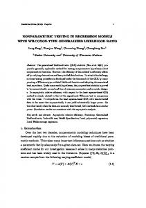
Figure 1 plots the ratio of m ^ H2 (xj ; aj ) to m ^ H1 (xj ; aj ) for DGPs 1-2 and n = 100; 400, where (r) 1 P250 ^ Hl (xj ; aj ) for l = 1; 2; and j = 1; 2; :::; 225: In theory, both m ^ H1 (xj ; aj ) m ^ Hl (xj ; aj ) 250 r=1 m

and m ^ H2 (xj ; aj ) converge to m (xj ; aj ) in probability so that the points (m ^ H1 (xj ; aj ); m ^ H2 (xj ; aj )) should lie on the 45 degree line as n ! 1: Nevertheless, we see some discrepancies between

m ^ H1 (xj ; aj ) and m ^ H2 (xj ; aj ) for both DGPs and sample sizes. Clearly, the discrepancy is much larger for DGP 1 than that for DGP 2 for both sample sizes.

20

( b) D G P 1, n = 400

0 .8

0 .8

0 .6

0 .6

0 .4

0 .4

0 .2

0 .2 H2

1

0

m

m

H2

( a) D G P 1, n = 100 1

0

- 0 .2

- 0 .2

- 0 .4

- 0 .4

- 0 .6

- 0 .6

- 0 .8

- 0 .8

-1 - 0 .8

- 0 .6

- 0 .4

- 0 .2

0 m

0 .2

0 .4

-1 -1

0 .6

- 0 .8

- 0 .6

- 0 .4

0 .6

0 .6

0 .4

0 .4

0 .2

0 .2 H2

1 0 .8

0

m

H2

m

1

- 0 .2

- 0 .4

- 0 .4

- 0 .6

- 0 .6

- 0 .8

- 0 .8

-1

-1

- 0 .4

- 0 .2

0 m

0 .2

0 .4

0 .4

0 .6

0 .8

0

- 0 .2

- 0 .6

0 .2

H1

( d) D G P 2, n = 400

0 .8

- 0 .8

0 m

( c ) D G P 2, n = 100

-1

- 0 .2

H1

0 .6

0 .8

1

-1

- 0 .8

- 0 .6

- 0 .4

- 0 .2

0 m

H1

0 .2

0 .4

0 .6

0 .8

1

H1

Plots of m ^ H2 over m ^ H1 for DGPs 1-2: the solid line is the 45 degree line, the points for (m ^ H1 ; (r)

(r)

m ^ H2 ) on the dotted line are obtained as averages of (m ^ H1 (xj ; aj ) ; m ^ H2 (xj ; aj )), r = 1; :::; 250; over 250 replications

7.2

Speci…cation Testing

To examine the …nite-sample properties of the speci…cation test, we consider the two DGPs: 2

DGP 3: Yi = (0:5 + 0:1Xi2 )Ai + 2 0 Xi =(0:1 + eAi =2 ); DGP 4: Yi =

((Xi + 1)Ai =4) (Xi + 1)

0:5 0 Ai =(1 + Xi2 );

where i = 1; :::; n; and Ai ; Xi and Zi are generated as in DGPs 1-2. Note that when

0

= 0;

DGPs 3 and 4 reduce to DGPs 1 and 2, respectively, permitting us to study the level behavior of our test. For other well-chosen values of

0;

m (x; a) as de…ned in DGP 3 or 4 is not strictly

monotonic in a; permitting study of the test’s power against non-monotone alternatives. ^ p;b (Yi jXi ; z) and G ^ 1 (G ^ p;b (Yi jXi ; z) j To construct the raw test statistic J^n , we …rst obtain G p;b

21

DGP 3

Table 2: Finite sample rejection frequency for DGPs 3-4 Warp-speed bootstrap Full bootstrap 0

n 100 200

4

100 200

0 1 0 1

1% 0.018 0.320 0.020 0.392

5% 0.042 0.388 0.060 0.442

10% 0.124 0.420 0.148 0.474

1% 0.008 0.316 0.020 0.408

5% 0.080 0.404 0.076 0.464

10% 0.140 0.456 0.140 0.508

0 1 0 1

0.014 0.288 0.004 0.356

0.032 0.576 0.014 0.564

0.068 0.660 0.036 0.688

0.016 0.456 0.008 0.476

0.032 0.656 0.012 0.712

0.056 0.724 0.056 0.792

x ; z) by choosing the order of the local polynomial regression, the kernel function K; and the bandwidth b: As when estimating the response, we choose p = 1 and let K be the product of univariate standard normal PDFs. Since we require undersmoothing for our test, we set b = (c2 SX n

1=5 ;

c2 SZ n

1=5 );

where c2 is a positive scalar that we use to check the sensitivity of our test

to the choice of bandwidth. Next, we need to choose weight functions H1 ; H2 ; and : We choose H1 and H2 as above and set 0 ;X

0 th

sample quantile of

0 ;X

Xi

1

0 ;X

1

0 ;Y

Yi

1

0 ;Y

;

fXi gni=1

and 0 = 0:0125: These sample quantiles p converge to their population analogs at the parametric n rate, so they can be replaced by the ^ p;b and G ^ 1 in the tails. latter in deriving the asymptotic theory. By construction, we trim G p;b where, e.g.,

is the

(Xi ; Yi ) = 1

= SZ n 1=6 ; x = SX n 1=6 ; and a = SA n 1=6 ; where, e.g., SA is the sample standard deviation of A^i : For computational feasibility, we consider two sample In the bootstrap, we set

z

sizes, n = 100; 200; in our simulation study. Also for computational feasibility, for each sample size n; our “full”bootstrap experiments use 250 replications and B = 100 bootstrap resamples in each replication. Before performing the full bootstrap with B = 100, we study the sensitivity of the test to the bandwidth b = (c2 SX n

1=5 ;

c2 S Z n

1=5 )

as suggested by Giacomini, Politis, and

White (2007), using their warp-speed bootstrap. In this procedure, only one bootstrap resample is drawn in each replication. Because of its relatively low computational cost, we can use 500 replications for this study. We …nd that our test is not very sensitive to the choice of b as long as c2 is not too big or small. For example, the test behaves reasonably well for c2 lying between 1 and 2. Table 2 reports the warp-speed bootstrap results for the case c2 = 1:5; together with the full bootstrap results for c2 = 1:5 with B = 100. Table 2 reports the empirical rejection frequencies for our test at various nominal levels for DGPs 3-4. The rows with

0

= 0 report the empirical level of our test; those with

0

= 1 show

empirical power. We summarize the main …ndings from Table 2 as follows: First, the level of our test is fairly well behaved, and it can be close to the nominal level for sample sizes as small as n = 100: When n increases, the level generally improves somewhat. Second, the power of

22

our test is reasonably good. It increases as the sample size doubles for both the warp-speed and full bootstrap methods. Finally, the full bootstrap tends to deliver somewhat better power performance than the warp-speed bootstrap, similar to …ndings of Cho and White (2011).

8

Empirical Applications

This section illustrates the usefulness of our tests with two examples. To show their broad applicability, we consider two very di¤erent applications. The …rst application analyzes an important question for policy analysis, namely the determinants of the Black-White earnings gap. The second application comes from a traditional area of economics: classical consumer demand using Engel curves. We discuss the economic background, provide details of the data and the test implementation, and discuss our …ndings.

8.1 8.1.1

The Black-White Earnings Gap: Just Ability? Economic Background

The quest for the sources of the apparent di¤erences in economic circumstances between the three major races in the US, i.e., Blacks, Hispanics, and Whites, has spurred an extensive and controversial debate over the last few decades. Starting with the seminal paper by Neal and Johnson (1996, NJ), a ‡ourishing literature has emerged that focuses primarily on the sources of the Black-White earnings gap; obviously, a key concern in this is the potential existence of racial discrimination, i.e., the fact that people with the exact same ability get di¤erential wages for the same task. Carneiro, Heckman, and Masterov (2005, CHM) give a recent overview of this literature, emphasizing the points important to our application. As NJ argue, to obtain a measure of the full e¤ect of discrimination in labor outcomes (e.g., wages) from a regression, one should not condition on variables that may indirectly channel discrimination, such as schooling, occupational choice, or years of work experience, as these may mask the full e¤ects. As CHM aptly put it, the “full force”of discrimination would not be visible. Chalak and White (2011a) contains supporting discussion of the “included variable bias” arising by conditioning on variables indirectly channeling a cause of interest. As argued convincingly in CHM, however, schooling is no longer a plausible channel of discrimination, given the extent of a¢ rmative action. Indeed, CHM show that when conditioned just on schooling, the wage gap increases, rather than decreasing, as would be the case if schooling were an indirect channel of discrimination. Thus, we include years of schooling as a causal factor in our analysis. The structural relation is then Y = m(X1 ; X2 ; A);

23

where A is work-related ability; X1 is years of schooling; X2 is race, a discrete variable taking three values; and Y is the wage an individual receives. As X and A are plausibly correlated, we seek a conditioning instrument Z such that X is independent of A given Z. To …nd this variable, we go back to the literature. NJ suggest the 1980 AFQT score as a proxy for ability. Once NJ condition on the AFQT, which we now denote Z, the maintained hypothesis is that there is no relationship between X and A, that is, X ? A j Z. This means that whatever

is not exactly accounted for in A by using Z does not correlate with race or schooling, in line with

NJ. Their …nding (corroborated by the analysis in CHM, with the additional schooling variable) of an absence of a Black (X2 = 1) E [m(X1 ; 1; A)jX1 ; Z]

White (X2 = 0) earnings gap means in our notation that

E [m(X1 ; 0; A)jX1 ; Z] = 0: This evidence is consistent with the absence

of discrimination in the labor market. Nevertheless, this is not the only testable implication of their hypotheses. We can now test the null hypothesis that there is indeed only a single unobservable that monotonically drives wages. Accordingly, we de…ne ability as a scalar factor that drives up wages for all values of X = x. As such, scalar monotonicity is a natural assumption - the more able somebody is, the higher his wage is, ceteris paribus. The fact that we can apply this logic here hinges on the Z variable, AFQT80, which is chosen to ensure unconfoundedness. The alternative is that there is some more complex mechanism that generates wage outcomes. There are a number of reasons why there may be a more complex relationship. One is that discrimination acts through several unobserved channels; another is what CHM have argued, namely that there are unobserved (in their data, actually at least partially observed) factors in the early childhood of an individual that have a large impact on labor market outcomes, and that should be accounted for. With the data at hand, we cannot separate these two explanations; however, we can shed light on whether a scalar “ability” accounts for observed outcomes. 8.1.2

The Data

Our data come from NJ’s original study,6 which is based on the National Longitudinal Survey of Youth (NLSY). The NLSY is a panel data set of 12,686 youths born between 1957 and 1964. This data set provides us with information on schooling, race, and labor market outcomes. The Z variable is the normalized AFQT80 test score, i.e., the armed forces test in 1980. Individuals already in the labor market have been excluded. The test score is also year-adjusted and then normalized to have mean 0 and variance 1 as in NJ. After cleaning the data, we have 3,659 and 3,783 valid observations for the female and male subsamples, respectively, and following the literature, we analyze men and women separately. Since the data set is quite large and the computational requirements exceed what we can handle on our computers, we divide each subsample into three sub-subsamples to obtain 1,220 + 1,220 + 1,219 female observations, and 6

Indeed, our data are exactly NJ’s original data; we are indebted to Derek Neal for providing us with this.

24

1,261+1,261+1,261 male observations. These subpopulations were selected randomly by taking every third observation in each group. Since we are otherwise using exactly the same data as NJ, we refer to their paper for summary statistics and other data details. 8.1.3

Implementation Details

The details of the testing procedure we implement are largely identical to those for the simulation study of Section 6.2. The kernel is the product of univariate standard normal PDFs; the order of the local polynomial is 1. The bandwidth is chosen by the rule of thumb in Section 6.2, paragraph 2. We perform 200 bootstrap replications; with n

1; 200; each replication takes about two hours

using Matlab code running on modern high-speed processors. 8.1.4

Empirical Results

The values of the test statistics we obtain using the procedures described above are 9.381, 12.633, and 85.119 for the three female subsamples, and 250.24, 140.55, and 246.85 for the male subsamples. The associated p-values are 0.995, 1, and 0.815 for the three female subsamples, and 0.510, 0.925, and 0.720 for the three male subsamples. Obviously, the fact that we have drawn subsamples reduces the power of our procedure. But increasing the sample size even moderately increases the processing time for each bootstrap replications to signi…cant multiples of the two hours required with n

1; 200: Nevertheless, since the test statistic values are so far from

the critical values and the p-values are so large, we believe it safe to conclude that the null of scalar monotonicity is not rejected. This is evidence consistent with the correct speci…cation of the NJ/CHM model. Of course, further research with better data is required to analyze the importance of early childhood education as CHM suggest, but this is beyond our scope here. Recall that we maintain conditional exogeneity, B:1. Without this, the test is a joint test for A:2 and B:1: Under this interpretation, we have no evidence against either A:2 or B:1: To illustrate use of a multiple test for misspeci…cation, we also report the results of a pure test of B:1: By White and Chalak (2010, prop.2), we can test B:1 by testing X ? S j Z; where S = q(Z; A; V ); with

X ? V j (A; Z): A plausible candidate for S is another proxy for A; viewing V as a measurement error. Here, a natural choice for S is the 1989 AFQT score. To implement, we standardize

AFQT89 in the same way as AFQT80, and we apply the conditional independence test of Huang and White (2010). The table below reports the results for each of the samples described above. For none of these do we reject B:1; consistent with our monotonicity test …ndings.

p-value

Sample 1

Male Sample 2

Sample 3

.80

.28

.20

25

Sample 1

Female Sample 2

Sample 3

.39

.88

.85

8.2 8.2.1

Engel Curves in a Heterogeneous Population Economic Background

Engel curves are among the oldest objects analyzed by economists.7 Modern econometric Engel curve analysis assumes that Y = m(X1 ; X2 ; A);

(8.1)

where Y is a K-vector of budget shares for K continuously-valued consumption goods; X1 is wealth, represented by (log) total expenditure under the assumption that preferences are timeseparable; X2 denotes observable factors that re‡ect preference heterogeneity; and A denotes unobservable preference heterogeneity. Prices are absent here, as Engel curve analysis involves a single cross section only, and prices are assumed invariant. However, it is commonly thought that log total expenditure is endogenous8 and is hence instrumented for, typically by labor income, say S: This is justi…ed by the same intertemporal separability assumption. Here, we follow IN, and write the X1 structural equation as X1 = (S; X2 ; Z);

(8.2)

where the unobserved drivers of X1 are denoted Z. For simplicity, we assume X2 is exogenous. Following IN, we also assume S is exogenous, so we take (S; X2 ) ? (A; Z); implying (X1 ; X2 ) ? A j Z. With the usual normalization, Z j (S; X2 ) is U[0; 1]; and Z is identi…ed as Z = F (X1 j S; X2 ):

(8.3)

IN’s control function approach thus provides us with a variable Z that satis…es our assumptions. We are now able to test the hypothesis that there is a single unobservable A in equation (8.1) that enters monotonically. Put di¤erently, due to the tight relationship between quantiles and nonseparable models with monotonicity, we can test whether in the conditional -quantile regression of Y on X and Z, the parameter

can be given a structural interpretation. The alternative is that

there is a more complex structure in the unobservables. An example of a structural model that assumes monotonicity is provided in Blundell, Chen, and Kristensen (2007), who assume Y = m(X1 ; X2 ) + A: Nevertheless, to test this speci…cation, we also must specify equation (8.2) as above. 7

They were …rst analyzed in1857 by the Saxonian economist Ernst Engel (1821–1896), not to be confused with Friedrich Engels, the companion of Karl Marx. 8 Nevertheless, the evidence is not strong; see Blundell, Horowitz, and Parey (2009) or Hoderlein (2010).

26

8.2.2

The Data

For our test, we use the British FES in exactly the form employed in IN.9 The FES reports a yearly cross section of labor income, expenditures, demographic composition, and other characteristics of about 7,000 households in every year. Since we are considering Engel curves, we use only the cross section for 1995. We focus on households with two adults, where the adults are married or cohabiting, at least one is working, and the household head is aged between 20 and 55. We also exclude households with 3 or more children. This yields a sample with n = 1; 655: This will be our operational subpopulation, not least because it is the one commonly used in the parametric demand system literature; see Lewbel (1999). The expenditures for all goods are grouped into several categories. The …rst is related to food consumption and consists of the subcategories food bought, food out (catering), and tobacco. The second and third categories contain expenditures related to alcohol and catering. The alcohol category is probably mismeasured, so we do not employ it as dependent variable. The next group consists of transportation categories: motoring, fuel expenditures, and fares. Leisure goods and services are the last category. For brevity, we call these categories Food, Catering, Transportation, and Leisure. We work with these broader categories since more detailed accounts su¤er from infrequent purchases (recall that the recording period is 14 days) and are thus often underreported. Together these account for approximately half of total expenditure, leaving a large fourth residual category. Labor income is as de…ned in the Household Below Average Income study (HBAI). Roughly, this is net labor income to the household head after taxes, but including state transfers. The following table gives some summary statistics; for more details, see Hoderlein (2010). Variable

Food

Catering

Alcohol

Transport

Leisure

LogExp

LogWage

nKids

Mean

0.2074

0.0805

0.0578

0.2204

0.1297

5.4215

5.8581

0.6205

8.2.3

Implementation Details

To apply the test, we let Y be the budget shares of Food, Catering, Transportation, or Leisure in (8.1).10 In each case, we specify X1 as the logarithm of total expenditure and X2 as the number of kids in a family. The details of the testing procedure are again largely identical to those implemented in the simulation study in Section 6.2 and in the previous application. We use a product kernel and select the bandwidth by the same rule of thumb as in Section 6.2, paragraph 2. Again, we performed 200 bootstrap replications, each of which takes approximately 3.3 hours. The major di¤erence is that the instrument Z = F (X1 j S; X2 ) must be estimated from the

data in a …rst stage. To mitigate the bias from the …rst stage, we use local quadratic regression, 9

We are grateful to Whitney Newey and Richard Blundell for providing us with the data. We did not consider the budget share for alcohol because there are too many 0 observations (258 out of 1,665) in the data. 10

27

employing a Gaussian kernel and Silverman’s rule-of-thumb bandwidth. Standard U -statistic theory straightforwardly shows that the variance term in the decomposition of the di¤erence between Z and its estimate will not a¤ect the asymptotic null distribution of our test statistic. Consequently, the Tn statistic based on estimated Z is asymptotically equivalent to that based on the true unobservable Z under the null and some side conditions. This behavior is well known in the literature on nonparametrically estimated regressors, so to conserve space, we do not provide formal details. Using estimated Z also has implications for the bootstrap. Ideally, one would prefer a bootstrap method alternative to that applied here, based entirely on observables, while imposing the null. Developing and justifying this is a substantive undertaking, deserving of a paper in itself. We therefore leave this as a topic for future research. 8.2.4

Empirical Results

The following table summarizes our test results:

Value of Test Statistic

Food

Catering

Transportation

Leisure

1:2895

0:7336

1:5905

1:1492

0:005

0:005

0:005

0:010

p-values

Two things are noteworthy. First, observe that rather small values of the test statistic are associated with small p-values. This indicates that the normal approximation is a poor description of the true …nite-sample behavior, a result that is quite familiar in the nonparametric testing literature. Second, in all four categories analyzed, we soundly reject the null of monotonicity. The rejections are strongest in Food, Catering, and Transportation, and slightly less pronounced for Leisure. Whereas in the labor application above it seems conceivable that there is only one major omitted unobservable, i.e., ability, our test here suggests that this is not a valid description of the unobservables driving consumer behavior. This should not be surprising, given that consumer demand is usually thought to be a result of optimizing a rather complex preference ordering, given a budget set. Still, empirically establishing this fact, uniformly over a number of expenditure categories, is encouraging evidence of the ability of our test to produce economically interesting results in real-world applications.

9

Concluding Remarks

Monotonicity in unobservables is a now common assumption in applied economics. Its appeal arises from the fact that it allows one to recover the unknown structural function from the regression quantiles of the data. As we discuss, monotonicity is a strong assumption, and its failure has substantive consequences for structural inference.

28

So far, there are no generally applicable nonparametric speci…cation tests designed to detect monotonicity failure. This paper provides such a test for cross-section data. We show how to exploit the power of an exclusion restriction together with a conditional independence assumption, plausible in a variety of applications, to construct a test statistic. We analyze the large-sample behavior of our estimators and tests and study their …nite-sample behavior in Monte Carlo experiments. Our experiments show that a suitable bootstrap procedure yields tests with reasonably well behaved levels. Both theory and experiment show that the test has useful power. When applied to data, the test exhibits these features. In a labor economics application where monotonicity in unobserved ability is plausible, we …nd that the test does not reject. In a consumer demand application, where monotonicity in a scalar unobserved preference parameter is less plausible, we …nd that the test clearly rejects. These two distinct applications also illustrate that our test applies to both observed and unobserved conditioning instrument cases and works well in both. Finally, we expect that our approach, or elements thereof, extends to tests for monotonicity in richer economic structures such as in Olley and Pakes (1996), but we leave this, in our opinion fascinating, extension for future research.

10

Mathematical Appendix

Proof of Theorem 3.2: Let ( ) A ! V: By assumption,

m(x; ) : A ! R: Clearly, (a) takes values in V; so ( ) :

is measurable and strictly increasing, so its inverse function

V ! A exists and is measurable and strictly increasing. Let m : X

m( ( );

1(

):

V ! R be de…ned as m( ; )

)); where ( ) is the identity map. This is the composition of m with the measurable

map # : X #2 (x; v) =

V!X

1 (v):

A; de…ned by #(x; v) = (#1 (x; v); #2 (x; v)); where #1 (x; v) = (x); and

As compositions of measurable functions are measurable, m : X

V ! R is

(product) measurable.

(a) Let x 2 X be arbitrary.

m(x;

1(

1 (v))

Take any v 2 V; and put a =

1 (v):

Then m(x; a) =

= m(x; v); as desired. The argument for the second claim is similar.

(b) By assumption, m(x; ) is strictly increasing on A, and by construction,

1

is strictly

increasing on V. Because compositions of strictly increasing functions are strictly increasing, it

follows that m(x; ) = m(x;

1(

)) is strictly increasing on V:

(c) For each v in V; there exists a =

m(x;

1 (v))

1 (v)

such that v = (a) = m(x; a) = m(x;

1[

(a)]) =

= m(x; v):

Proof of Theorem 3.3 A:0, A:1; and B:1 ensure that for all (y; x; z) G(yjx; z)

P [Y

yjX = x; X = z] = P [m(X; A)

yjX = x; Z = z] = P [m(x; A)

yjZ = z]:

Setting y = m(x; a); it follows from B:2 that for all a; x; z m(x; a) = G

1

(P [m(x; A) 29

m(x; a)jZ = z] j x; z):

(10.1)

Pick any (a; x; x ~; z) 2 A G

X

X

Z:

(a) We show that (i) implies (ii) : a 2 mx~ 1 fG

1 (G(m(~ x; a)

1 [G(m(x; a)

j x; z) j x ~; z]g: By B:2; m(x; a) =

jx ~; z) j x; z) implies G(m(x; a) j x; z) = G(m(~ x; a) j x ~; z); and m(~ x; a) = G

1

[G(m(x; a) j x; z) j x ~; z]:

Taking the pre-image mx~ 1 gives the desired result. (b) We show that (ii) implies (i): By the de…nition of the pre-image, a 2 mx~ 1 fG

x; z) j x ~; z]g implies

m(~ x; a) = G

1

1 [G(m(x; a)

[G(m(x; a) j x; z) j x ~; z]:

Invoking B:2 to invert G twice, we obtain the desired result. (c) We show that (i) implies (iii): Given (i); we have m(x; a) = G

1

= G

1

= G

1

(P [m(X; A)

m(~ x; a) j X = x ~; Z = z] j x; z)

= G

1

(P [m(~ x; A)

m(~ x; a) j X = x ~; Z = z] j x; z)

= G

1

(P [m(~ x; A)

m(~ x; a) j Z = z] j x; z);

(G(m(~ x; a) j x ~; z) j x; z) (P [Y

m(~ x; a) j X = x ~; Z = z] j x; z)

where the last step follows from B:1. Using this result and (10.1) ensures that G

1

(P [m(x; A)

By the invertibility of G P [m(x; A)

m(x; a)jZ = z] j x; z) = G 1

1

(P [m(~ x; A)

m(~ x; a) j Z = z] j x; z):

ensured by B:2, it follows that m(x; a)jZ = z] = P [m(~ x; A)

P [A 2 mx 1 fm(x; a)gjZ = z] = P [A

m(~ x; a) j Z = z]

or

x; a)g j Z = z], mx~ 1 fm(~

as desired. (b) We show that (iii) implies (i): Thus, suppose that P [A 2 mx 1 fm(x; a)gjZ = z] = P [A P [m(x; A)

mx~ 1 fm(~ x; a)g j Z = z]

m(x; a)jZ = z] = P [m(~ x; A)

m(~ x; a) j Z = z]:

Applying (10.1), the equality above, and B:2 gives m(x; a) = G

1

(P [m(x; A)

m(x; a)jZ = z] j x; z)

= G

1

(P [m(~ x; A)

m(~ x; a) j Z = z] j x; z):

30

or

j

Applying B:1 and simplifying gives m(x; a) = G

1

(P [m(~ x; A)

= G

1

m(~ x; a) j X = x ~; Z = z] j x; z)

(P [m(X; A)

= G

1

m(~ x; a) j X = x ~; Z = z] j x; z)

(P [Y

= G

1

(G(m(~ x; a) j x ~; z) j x; z):

m(~ x; a) j X = x ~; Z = z] j x; z)

Proof of Corollary 3.4 A:2 ensures Theorem 3.3(iii) for all (a; x; x ~; z): This ensures m(x; a) = G

1 (G(m(~ x; a)

jx ~; z) j x; z): Letting x ~ = x with a = m(x ; a) gives m(x; a) = G

x; z); ensuring (3.1). Successively inverting Y = G

1 (G(A

1 (a

j x ; z) j

j x ; z) j X; z) for any z gives (3.2).

Next, Y = m(X; A), X ? A j Z; and strict monotonicity imply that for all y; x; and z; G(y j x; z)

P[ Y

y j X = x; Z = z]

= P [ m(X; A)

y j X = x; Z = z] = P [m(x; A)

= P [ m(x; A) Setting y = m(x; a) so that a = m

y j Z = z] = P [ A 1 (x; y)

1

m

y j X = x; Z = z]

(x; y) j Z = z]:

(10.2)

immediately gives

FAjZ (a j z) = G( m(x; a) j x; z): We have FAjZ (a j z) = FAjX;Z (a j x; z) since X ? A j Z: This establishes eq.(3.3). Finally, for all (a; x; z) 2 A P[ A

X

Z;

a j X = x] = P [ m(x; A) = P [ m(X; A) = P [Y

1

[G(a j x ; z) j x; z] j x):

For the next results, recall that U0

dK

(u=b) ; and

p;b (u)

m(x; a) j X = x]

m(x; a) j X = x] = GY jX (m(x; a) j x)

= GY jX ( G b

m(x; a) j X = x]

p (u=b) :

Let Wi

X0

(Xi0 ; Zi0 )0 ; u

Z 0 ; Ui

(x0 ; z 0 )0 ; Kb (u)

(y; u0 )0 : Let Sp;b (u) and Sp;b (u)

(Yi ; Ui0 )0 and w

be as de…ned in (5.3) and (6.1), respectively. De…ne n

Vp;b ( ; u) Vp;b ( ; u) Bp;b (y; u) Vp;b (y; u)

1X Kb (Ui n

u)

p;b (Ui

u)

(Yi

Kb (Ui

u)

p;b (Ui

u)

Yi

Kb (Ui

u)

p;b (Ui

u)

Kb (Ui

u)

p;b (Ui

u) 1y (Wi ) ;

1 n 1 n 1 n

i=1 n X i=1 n X i=1 n X i=1

31

i;y

(u) ;

b(

G

1

; u)) ; ( jUi ) ;

where

(u)

1y (Wi )

1 fYi

1 (u yg

0) ;

i;y

(u)

G (yjUi )

G (yju)

P

1 (j) 1 jjj p j! G (yju) (Ui

u)j ; and

G (yjUi ) : Let Uis and us denote the sth elements of Ui and u.

To prove Theorem 5.1, we …rst establish some technical lemmas. Let Sp;b (u)

E[Sp;b (u)]

E[Bp;b (y; u)]: The next lemma establishes uniform consistency of ^ (yju) : p Lemma 10.1 Suppose that Assumptions C.1-C.4 and C.6 hold. Then with b n 1=2 b d=2 log n; we have that uniformly in (y; u) 2 R U0 ; (a) ^ (yju) (yju) = Sp;b (u) 1 [Vp;b (y; u) + Bp;b (y; u)] + OP ( 2b + b bp+1 ); (b) ^ (yju) (yju) = OP ( b + bp+1 ): and Bp;b (y; u)

Proof. Since [Sp;b (u)]

1

Sp;b (u) = IN where IN is an N

N identity matrix, by (5.2) we

obtain the following standard bias and variance decomposition: ^ (yju)

1

(yju) = [Sp;b (u)]

Vp;b (y; u) + [Sp;b (u)]

1

Bp;b (y; u) :

(10.3)

By Theorems 2 and 4 in Masry (1996) with some modi…cation to account for the non-compact support of the kernel function,11 Bp;b (y; u) = OP ( p bp+1 ); (10.4)

Sp;b (u) = Sp;b (u) + OP ( b ) ; Vp;b (y; u) = OP ( b ) ; Bp;b (y; u)

where the probability orders hold uniformly in u 2 U0 : By the same argument as used in the proof of Theorem 4.1 of Boente and Fraiman (1991), we can show that the last two results in (10.4) also hold uniformly in y 2 R under Assumption C.3. In addition, by the Slutsky lemma, Sp;b (u)

1

It follows that ^ (yju) = Sp;b (u)

1

= Sp;b (u) + Sp;b (u) (yju) = fSp;b (u)

[Vp;b (y; u) +Bp;b (y; u)] + OP (

Sp;b (u)

1

= [Sp;b (u)]

1

+ OP ( b ) :

(10.5)

1

+ OP ( b )gfVp;b (y; u) +[Bp;b (y; u) +OP ( b bp+1 )]g

2 b

+ b bp+1 ) = OP (

b

+ bp+1 ):

^ p;b (yjx; z) = e0 ^ (yju) where e1;p is de…ned after (5.3). Noting that uniformly in Recall that G 1;p (y; u) 2 R U0 ; Sp;b (u) = g (u) Sp +O (b) ; and Bp;b (y; u) = bp+1 g (u) Bp Gp+1 (yju)+o bp+1 ; with p+1 ; we have G ^ p;b (yju) G(yju) = bp+1 e0 S 1 Bp Gp+1 (yju) + g (u) 1 e0 S 1 Vp;b (y; u) + b b+b 1 p

1 p

OP (b b ): Lemma 10.2 Suppose that Assumptions C.1-C.4 and C.6 hold. Let T be any compact subset of (0; 1) : Then uniformly in ( ; u) 2 T U0 ; ^ 1 ( ju) G 1 ( ju) = e0 Sp;b ( ; u) 1 Vp;b ( ; u) + OP ( 2 + b bp+1 ) + oP n 1=2 b dX =2 ; (a) G 1;p b p;b ^ 1 ( ju) G 1 ( ju) = e0 Sp;b ( ; u) 1 Vp;b ( ; u) + bp+1 e0 Sp 1 Bp G 1 ( ju) + OP ( 2 ) + (b) G p;b

1;p

1;p

p+1

b

oP bp+1 + n 1=2 b dX =2 ; ^ 1 ( ju) G 1 ( ju) = e0 Sp ( ; u) 1 Vp;b ( ; u) [1 + oP (1)] + bp+1 e0 Sp 1 Bp G 1 ( ju) + (c) G 1;p 1;p p+1 p;b oP bp+1 + n 1=2 b dX =2 ; where Sp ( ; u) Sp g G 1 ( ju) ju g (u) is the limit of Sp;b ( ; u) E [Sp;b ( ; u)] :

11 The compact support of the kernel function in Masry (1996) can be easily relaxed, following the line of proof in Hansen (2008, Theorem 4).

32

Proof. Noting that Sp;b ( ; u)

Sp;b ( ; u) = OP ( b ) and Vp;b ( ; u) = OP (

b

+ bp+1 ) by

the proof of (b) below, (a) follows from Theorem 2.1 of Su and White (2011). To prove (b), 1 Pn G 1 ( jUi ) write Vp;b ( ; u) = Vp;b ( ; u) + Rp;b ( ; u) ; where Rp;b ( ; u) i=1 f1 Yi n

1(Yi

b(

; u)0

fRp;b ( ; u)

iu )gKb (Ui

u)

iu

and

p;b (Ui

iu

u) : Write Rp;b ( ; u) as E[Rp;b ( ; u)] +

E[Rp;b ( ; u)]g : The …rst term is

E[Rp;b ( ; u)] = E

1

G(G

= E g(G = bp+1 g(G

1

( jUi ) jUi )

G( 1

( jUi ) jUi ) G

1

b(

( jUi )

; u)0

iu jUi )

Kb (Ui

0

b(

; u)

u)

iu

Kb (Ui

iu

u)

f1 + o (1)g

iu

1 ( ju) ju)g (u) Bp Gp+1 ( ju) f1 + o (1)g :

It is easy to show the second term is oP (bp+1 ) uniformly in ( ; u). Thus (b) follows. For (c), it p su¢ ces to show that sup( ;x)2T U0 kSp;b ( ; u) Sp ( ; u)k = OP (n 1=2 b d=2 log n + b) = oP (1) : The proof is similar to but simpler than that of Corollary 2 in Masry (1996) because we only need convergence in probability, whereas Masry proved almost sure convergence. If G (ajx ; z) 2 T0 = [ ; ]

(0; 1) for x 2 X0 and all (a; z) 2 AH

Z0 ; by Lemma 10.1,

^ p;b (ajx ; z) 2 T with probability approaching 1 for su¢ ciently large n; where T G 0 0 (0; 1) for some

[

> 0: Then the result in Lemma 10.2 holds uniformly in ( ; u) 2 T0

; + ]

U0 :

Lemma 10.3 Suppose that Assumptions C.1-C.4 and C.6 hold. Then p sup~; 2T0 ;j~ j M vb supu2U0 nbdX kVp;b (~; u) Vp;b ( ; u)k = oP (1). Vp;b ( ; u)) where ! 2 RNp with k!k = 1: We need

Proof. Let W (~; ; u) = ! 0 (Vp;b (~; u) to show that sup ~; 2T0 ;j~

sup jW (~; ; u)j = oP (#n ) with #n = n

1=2

b

dX =2

:

(10.6)

j M vb u2U0

u) =b) ! 0 p;b (Ui u) ; a+ i;u = max (ai;u ; 0) and ai;u = max ( ai;u ; 0) : Noting P 1 n that W (~; ; u) = nbd 1 Yi G 1 (~jUi ) + 1 Yi G 1 ( jUi ) ; we can i=1 ai;u ~

Let ai;u = K ((Ui

analogously de…ne W + (~; ; u) and W (~; ; u) by replacing ai;u in the de…nition of W (~; ; u) by a+ i;u and ai;u ; respectively. By the Minkowski inequality, (10.6) will hold if sup~; jW + (~;

; u)j = oP (#n ) and sup~;

2T0 ;j~

j M vb

show the …rst part as the other case is similar. Let en

n

1=2 :

2T0 ;j~

Ul = fu : ku

ul k

Wn1 + Wn2 ; where

supu2U0

supu2U0 jW (~; ; u)j = oP (#n ) : We will only

By selecting n1 = O en 1 grid points,

1


#n

0

bdZ 20 p n 1=2 b d=2 log n + n

C4

k ; ul )

1=2 b dX =2

0

0

!

= o (1) ;

where Ci ; i = 1; 2; 3; 4; are positive constants. Thus Wn11 = oP (#n ) : By the monotonicity of the indicator and quantile functions and the nonnegativity of a+ i;ul , we can readily show that Wn12 =

max

1 l n2

+1 Yi

max

1 j;k n1 j j kj M

G

1

~2Tj ; 2Tk b j~ j M b

a+ i;ul

( jUi ) ]

max sup

1 l n2 ; ~2Tj 1 j n1

n 1 X + ai;ul [~ nbd

sup

j

1=2

1 Yi 1 Yi

G

1 Yi

1

G

i=1

n 1 X + + max sup ai;ul 1 l n2 ; 2Tk nhd

= OP (n

1

G

i=1

n 1 X + ai;ul ~ nhd

G

i=1

1 j n1

1 Yi

1

( j jUi )

(~jUi )

1

( jUi )

(~jUi )

k

j

+ 1 Yi

+ 1 Yi

k

G

1 Yi

1

G 1

k jUi )

( j jUi ) 1

G

(

(

k jUi )

) = oP (#n ):

We now study Wn2 : Assumption C.4(iii) implies that for all ku1 jK (u2 ) where K (u) = C1 (kuk

2d

K)

tion. For any u 2 Ul , ku

ul k =b

K (u1 )j

u2 k

K (u1 ) ;

for some constant C that depends on en : It follows from (10.7) that jKiu

34

K;

(10.7) 1

and Kiul j

2

in the assumpen Kiul where

Kiu

K ((Ui

ul )=b) and Kiul Ui

k

u

k

ul

Kiul

b

k

u

jkj en Kiul k)

Ui

Kiul j +

jKiu

b (2

ul )=b) ; and

Ui

Kiu

b Ui

K ((Ui

+ (2

k

u b

0 a+ i;ul = Kiu !

jkj 1 en Kiul 1 (jkj k)

p;b (Ui

Kiul ! 0

u)

ul b

> 0)

With this, we can show that for any u 2 Ul such that ku a+ i;u

Ui

ul k =b

p;b (Ui

ul )

k

Kiul

Cen (Kiul + Kiul ): en ; we have Cen (Kiul + Kiul ):

It follows that Wn2 =

max sup sup

1 l n2 u2Ul 2T ~;j~ 0

1

2 max sup nbd 1 l n2 u2Ul

Cen max

1 l n2

Thus we have proved that sup~;

W + (~; ; u)

sup j M n X

i=1 n 1X

nbd

W + (~; ; ul )

b

a+ i;u

a+ i;ul

Kiul + Kiul = OP (en ) = oP (#n ):

i=1

2T0 ;j~

j M vb

supu2U0 jW + (~; ; u)j = oP (#n ) :

By Lemmas 10.1 and 10.3, with probability approaching 1 we have p ^ p;b (ajx ; z); x; z Vp;b (G(ajx ; z); x; z) = oP (1) : nbdX Vp;b G sup (a;x;z)2AH X0 Z0

Proof of Theorem 5.1 Letting ^z R mH (x; a) = [G 1 (^z j x; z) G 1 (

z

Mn1 (x; a) + Mn2 (x; a) ; say. Note that G

1

(^z jx; z)

where r^ (a; x ; x; z)

g 0 (G g(G

G 1( 1(

1

^ p;b (ajx ; z) and z G G(ajx ; z), we have m ^ H (x; a) R ^ 1 (^z j x; z) G 1 (^z j x; z)]dH(z) j x; z)]dH(z) + [G p;b

( z jx; z) =

z jx;z)jx;z

z jx;z)jx;z)

) 3

(^z

g (G

^z 1(

2 z)

z z jx; z) jx; z)

and

z

+ r^ (a; x ; x; z) ;

lies between ^z and

mark after Lemma 10.1 and Assumption C.6, r^ (a; x ; x; z) = OP n oP n

1=2 b dX =2

1 b d log n

z:

By the re-

+ b2(p+1)

uniformly in (a; x; z) 2 AH X0 Z0 : It follows that for all (a; x) 2 AH Z p p ^z z d d nb X Mn1 (x; a) = nb X dH (z) + oP (1) 1 g (G ( z jx; z) jx; z) Z 0 p e1;p Sp;b (x ; z) 1 Bp;b (a; x ; z) = nbdX dH (z) g (G 1 ( z jx; z) jx; z) Z 0 p e1;p Sp;b (x ; z) 1 Vp;b (a; x ; z) d X + nb dH (z) + oP (1) g (G 1 ( z jx; z) jx; z) Mn11 (x; a) + Mn12 (x; a) + oP (1) ; say, 35

= X0

where the second line follows from Lemma 10.1(a). Noting that Bp;b (a; u) = E[Kb (Ui p;b (Ui

u)

i;a (u)]

in (a; u) 2 AH

u)

= bp+1 g (u) Bp Gp+1 (aju) + o bp+1 and Sp;b (u) = Sp g (u) + o (1) uniformly

U0 ; we have p

Mn11 (x; a) =

nbdX bp+1

Z

e01;p Sp 1 Bp Gp+1 (ajx ; z) dH (z) f1 + oP (1)g g (G 1 ( z jx; z) jx; z)

(10.8)

and p

Mn12 (x; a) =

where Mn12 (x; a)

nbdX

x; z~ p (~

z)

e01;p Sp 1 Vn (a; x ; z) dH (z) f1 + oP (1)g g (x ; z) g (G 1 ( z jx; z) jx; z) d

= Mn12 (x; a) f1 + oP (1)g ! N (0; V1 ) ; q R e01;p Sp 1 Kb (Xi x ;Zi z) p;b (Xi x ;Zi bdX Pn i=1

n

true uniformly in (a; x) 2 AH 0

Z

Sp 1 e1;p K

g(x ;z)g(G

X0 , V1

(~ x; z~) K (~ x; z~

1p

R

1(

z (1

g(x ;z)g(G

(10.9) z)1a (Wi )

z jx;z)jx;z) 2 z )h(z) 2 1( z jx;z)jx;z)

dH (z) ; (10.8) holds R 0 dz; 1p e1;p Sp 1 p (~ x; z~)

z) d (~ x; z~; z) ; and (10.9) follows from straightforward mo-

ment calculations and Liapounov’s central limit theorem. p For Mn2 ; noting that nbdX o(bp+1 + n 1=2 b dX =2 ) = o (1) under Assumption C.6, by Lemma 10.2 we have that uniformly in (a; x) 2 AH X0 Z p p 1 d d (^z jx; z) dH(z) nb X Mn2 (x; a) = nb X bp+1 e01;p Sp 1 Bp Gp+1 Z p + nbdX e01;p Sp (^z ; x; z) 1 Vn (^z ; x; z) dH(z) + oP (1) ; Mn21 (x; a) + Mn22 (x; a) + oP (1) ; say,

where Sp ( ; u) (a; x) 2 AH

Sp g G

1(

X0 Mn21 (x; a) =

ju) ju g (u) : By Lemmas 10.2 and 10.3, we have that uniformly in

p

nbdX bp+1

Z

1 ( z jx; z) dH(z) + oP (1) ; e01;p Sp 1 Bp Gp+1

and Mn22 (x; a) = Mn22 (x; a) + oP (1) ; where Mn22 (x; a) Furthermore, Mn22 (x; a) =

r d

where V2

1p

R

R

e01;p Sp ( z ; x; z)

n Z bdX X e01;p Sp 1 Kb (Ui u) p;b (Ui u) z Yi G n g (x; z) g (G 1 ( z jx; z) jx; z)

1

(10.10)

Vn ( z ; x; z)dH(z):

1(

z jUi )

dH (z)

i=1

! N (0; V2 ) ; z (1 g(x;z)g(G

2 z )h(z) 2 1( z jx;z)jx;z)

dz: The asymptotic normality result follows by the Cramér-

Wold device and the fact that the asymptotic covariance of Mn12 and Mn22 zero. In sum, we p d have nbdX fm ^ H (x; a) mH (x; a) Bm (x; a; x )g ! N 0; 2m (x; a; x ) ; where Bm (x; a; x ) and

2 (x; a; x m

) are de…ned in (5.6) and (5.7), respectively.

p Next, it is standard to show that sup(x;a)2X0 AH jMn12 (x; a)j = OP ( log n) and sup(x;a)2X0 p Mn22 (x; a) = OP ( log n): Then the uniform convergence result follows. 36

AH

Lemma 10.4 Suppose that Assumptions C.1-C.6 hold. Then for any n = O( b ); we have ^ p;b (a + n ju) G ^ p;b (aju) = g(aju) n + oP n + n 1=2 b dX =2 uniformly in u 2 U0 ; (a) G (b) m ^ H (x; a + n ) m ^ H (x; a) = DH (x; a) n + oP n + n 1=2 b dX =2 ; R g(ajx ;z) dH(z): where DH (x; a) g(G 1 (G(ajx ;z)jx;z)jx;z) Proof. By Lemma 10.1,

^ p;b (a + G

^ p;b (aju) = [G(a + G

n ju)

n ju)

G(aju)]

+e01;p Sp;b (u)

1

[Bp;b (a +

n ; u)

Bp;b (a; u)]

+e01;p Sp;b (u)

1

[Vp;b (a +

n ; u)

Vp;b (a; u)] + OP (

Clearly, the …rst term on the right hand side of the last expression is g(ajx; z) second term is

o(bp+1 )

= oP (n

1=2 b dX =2 )

2 b n

+

bb

p+1

):

+ o( n ); the

uniformly in u 2 U0 by the fact that Bp;b (a; u) =

bp+1 Bp Gp+1 (aju) g (u) + o bp+1 uniformly in u and Sp;b (u) = Sp g (u) + o (1), and the continuity of Gp+1 : Analogously to the proof of Lemma 10.3, we can show that Vp;b (a + oP (n

1=2 b dX =2 )

n ; u)

Vp;b (a; u) =

uniformly in u 2 U0 : Thus (a) follows.

To show (b), decompose m ^ H (x; a + n ) m ^ H (x; a) = Dn1 + Dn2 ; where Z h i ^ p;b (a + n jx ; z)jx; z)) G 1 (G ^ p;b (ajx ; z)jx; z)) dH(z); Dn1 G 1 (G

and

Z h

Dn2

For Dn1 ; we have Dn1 =

i ^ 1 (G ^ p;b (a + n jx ; z)jx; z)) G 1 (G ^ p;b (a + n jx ; z)jx; z)) dH(z) G p;b Z h i ^ 1 (G ^ p;b (ajx ; z)jx; z)) G 1 (G ^ p;b (ajx ; z)jx; z)) dH(z): G p;b

Z ^ Gp;b (a + g G

=

Z

g G

1

1

= DH (x; a)

n jx

; z)

^ p;b (ajx ; z) G

dH(z) + oP

n

+n

1=2

b

dX =2

g(ajx ; z) n dH(z) + oP ^ p;b (ajx ; z)jx; z jx; z G

n

+n

1=2

b

dX =2

^ p;b (ajx ; z)jx; z jx; z G

n

+ oP

n

+n

1=2

b

dX =2

;

where the …rst equality follows from the Taylor expansion, the second from (a), and the third from Lemma 10.1. By the proof of Theorem 5.1, we have Z h i 1 1 Dn2 bp+1 e01;p Sp 1 Bp Gp+1 (G(a + n jx ; z)ju) Gp+1 (G(ajx ; z)ju) dH(z) Z + e01;p [Sp (G(a + n jx ; z); x; z) 1 Vp;b (G(a + n jx ; z); x; z) Sp (G(ajx ; z); x; z)

Dn21 + Dn22 ; say. 37

1

Vp;b (G(ajx ; z); x; z)]dH(z)

It is easy to see that Dn21 = o(bp+1 ) = oP (n

1 by the continuity of G and Gp+1 : Next,

1=2 b dX =2 )

we write Dn22 = Dn22;1 + Dn22;2 ; where Z Dn22;1 = e01;p Sp (G(a+ n jx ; z); x; z) 1 [Vp;b (G(a+ n jx ; z); x; z) Vp;b (G(ajx ; z); x; z)] dH(z); Z Dn22;2 = e01;p [Sp (G(a+ n jx ; z); x; z) 1 Sp (G(ajx ; z); x; z) 1 ]Vp;b (G(ajx ; z); x; z) dH(z): One can readily show that Dn22;1 = oP (n

1=2 b dX =2 )

and Dn22;2 = oP (n

1=2 b dX =2 )

by standard

moment calculations and the dominated convergence theorem, and (b) follows. Proof of Theorem 5.3 By the strict monotonicity of mH (x; ) for all x; its inverse function mH 1 (x; ) exists and is unique. This implies that for any …xed (x; a) with y = mH (x; a) (and thus a = mH 1 (x; y)); there is an = ( ) = minfmH (x; a)

= (x) > 0 such that mH (x; a

) ; mH (x; a + )

mH (x; a)g > 0:

(10.11)

It follows that for su¢ ciently large n; m ^ H1 (x; y)

P

mH 1 (x; y) >

= P m ^ H1 (x; y) > mH 1 (x; y) +

or m ^ H1 (x; y) < mH 1 (x; y) or mH x; m ^ H1 (x; y) < mH x; mH 1 (x; y) - g

= P mH x; m ^ H1 (x; y) > mH x; mH 1 (x; y) + P

mH x; m ^ H1 (x; y)

mH x; mH 1 (x; y)

= P

mH x; m ^ H1 (x; y)

y >

mH x; m ^ H1 (x; y)

m ^ H x; m ^ H1 (x; y) )

= P P

(

sup jm ^ H (x; a)

a2AH

mH (x; a) j >

>

>

! 0;

where the third line follows from the monotonicity of mH (x; ) ; the fourth line holds by (10.11), ^ H x; m the …fth and six lines follow from the fact mH x; mH 1 (x; y) = y = m ^ H1 (x; y) ; and AH

fa : ja

Let

n (v)

cj P

for some c 2 AH g and n1=2 bdX =2

1 m

1

> 0:

(x; y) m ^ H1 (x; y)

mH 1 (x; y)

Bm

1

(x; y)

v 2 R: Then n (v)

= P m ^ H1 (x; y) = P = P

mH 1 (x; y) +

m ^ H x; m ^ H1 (x; y) m ^ H x; mH 1 (x; y)

n (v; x; y)

m ^ H x; mH 1 (x; y) + +

38

n (v; x; y)

y ;

n (v; x; y)

v

for any

where

n (v; x; y)

Bm

1

(x; y) + n

1=2 b dX =2

=P m ^ H x; mH 1 (x; y) (n =P

np h

!1 where

1=2

dX =2

b

(y; x) v: By Lemma 10.4(b) and Theorem 5.1,

DH x; mH 1 (x; y)

P m ^ H x; mH 1 (x; y)

n (v)

1

m

y + DH x; mH 1 (x; y) Bm )DH x; mH 1 (x; y)

nbdX DH x; mH 1 (x; y)

m ^ H x; mH 1 (x; y)

( v) =

n (v; x; y)

1

m

(x; y) o 1 (y; x) v

m 1

(y; x)

+y

1

y + DH x; mH 1 (x; y) Bm

(v) ;

1

i (x; y)

v

o

is the CDF for the standard normal distribution.

Proofs of Theorems 6.1 and 6.2 We prove Theorem 6.2, as Theorem 6.1 is a special case. Put R P ^ p;b (Yi jXi ; z) jx ; z)d (z)g2 i ; n ( ju) ^ 1 ( ju) G G = Gn ; and let Jn bdX ni=1 f G 1 (G p;b

G

1(

ju) ;

n1 (

; u)

G (Yi jXi ; z) ; and ^iz J^n = Jn + (J^n = Jn + bdX

e01 Sp;b ( ; u) 1 Vp;b ( ; u) ; and ^ p;b (Yi jXi ; z) : Noting that a2 G

Jn ) Z h n X i=1

+2b

dX

n Z h X i=1

= Jn + b

dX

^ 1 (^iz jx ; z) G p;b

^ 1 (^iz jx ; z) G p;b

Z n X

G

+2b +2b

dX

+2bdX

n Z X

i=1 n Z X

i=1 n Z X

1

i (^iz jx ; z) d

i (^iz jx ; z) d

1

2

n1 (^ iz ; x

; z) d

i=1

dX

G

n2 ( ; u) b2 = (a

n1 (^ iz ; x

n1 (^ iz ; x

; z) d

(z)

; z) d

(z)

n2 (^ iz ; x ; z) d

(z)

i=1

(z)

Z

+b

ju)

b) + 2 (a

n1 (

; u) ;

iz

b) b; we have

2

(z) Z

Z n X

i

G

1

(^iz jx ; z) d

(z)

i 2

n2 (^ iz ; x

; z) d

(z)

i

i=1

Z

Z

i

dX

(z)

n(

2

n2 (^ iz ; x

; z) d

(z)

i

G

1

(^iz jx ; z) d

(z)

i

G

1

(^iz jx ; z) d

(z)

i

Jn + J^n1 + J^n2 + 2J^n3 + 2J^n4 + 2J^n5 ; say.

(10.12)

We prove the theorem by …rst demonstrating that J^n = Jn + oP (1)

(10.13)

and then showing that Jn

d

Bn ! N 39

0;

2 J

;

(10.14)

where Jn

b

dX

"Z n X e01 Sp;b (Xi ; z) 1 Vp;b (Yi ; Xi ; z) + e01 Sp;b ( g (G 1 ( iz jx ; z) jx ; z)

iz ; x

1

; z)

Vp;b (

iz ; x

; z) d

#2

(z)

i=1

We prove (10.13) by showing that #2 "Z n X e01 Sp;b (Xi ; z) 1 Vp;b (Yi ; Xi ; z) dX Jn = b i + 0 + oP (1) ; g (G 1 ( iz jx ; z) jx ; z) i=1 Z n 2 X 1 dX 0 ^ Jn1 = b e1 Sp;b ( iz ; x ; z) Vp;b ( iz ; x ; z) d (z) i + oP (1) ;

i:

(10.15) (10.16)

i=1

J^n4 = J~n4 + oP (1) ;

and

(10.17)

J^ns = oP (1) for s = 2; 3; 5;

(10.18)

where J~n4

b

dX

n Z X e01 Sp;b (Xi ; z) 1 Vp;b (Yi ; Xi ; z) 0 e1 Sp;b ( g (G 1 ( iz jx ; z) jx ; z)

iz ; x

1

; z)

Vp;b (

iz ; x

; z) d

(z)

i:

i=1

To show (10.15), write Z n X dX Jn = b G +b

i=1 n X

Z

dX

+2b

i=1 n Z X

dX

(10.19)

2 1

(

iz jx

; z)d

(z)

i 2

G 1

G

1

G

1

(z)

Z

(^iz jx ; z)

(

iz jx

i=1

; z)d

(

iz jx

G

; z) d

1

(z)

(^iz jx ; z)

i

G

1

i

!

(

iz jx

; z) d

(z)

i

Jn1 + Jn2 + 2Jn3 ; say. Under H1 (

n)

with G

where r^i (z) = under H1 (

1

=n

n

1=2 b dX =2 ;

(^iz jx ; z)

g 0 (G g (G

n) ;

Jn3 = n

1

G

(

iz jx

; z) =

1 1

( iz jx ;z )jx ;z ) 3 (^ iz ( iz jx ;z )jx ;z )

1=2 dX =2

b

n X

i=1 n X

1

Jn1 = n

n (Xi ; Yi )

2 iz )

Z

Pn

^iz

g (G

1(

and

iz

G

Z

P

2 i=1 n (Xi ; Yi )

1

iz jx

iz

; z) jx ; z)

lies between

(^iz jx ; z)

G

1

(

1=2 dX =2

b

n (Xi ; Yi )

i=1

Jn31 + Jn32 ; say.

40

Noting that

+ r^i (z) ;

iz

iz jx

^iz iz d g (G 1 ( iz jx ; z) jx ; z) i=1 Z n X +n 1=2 bdX =2 (X ; Y ) r^i (z) d (z) i n i i

= n

0:

(10.20)

and ^iz ; we have that

; z) d

(z)

i

(z)

i

Observing that r^i (z) = OP n OP n

1 b d log n

Jn31 = n

1 b d log n

+ b2(p+1) uniformly in z; we have Jn32 = n1=2 bdX =2

+ b2(p+1) = oP (1). By Lemma 10.1 and Assumption C.6, we have

1=2 dX =2

b

n X

n (Xi ; Yi )

i=1

Z

Sp;b (Xi ; z) g (G 1 (

1

Vp;b (Yi ; Xi ; z) d iz jx ; z) jx ; z)

(z)

i

+ oP (1) :

Writing the dominant term in the last expression as a second order U-statistic plus a smaller order term (OP (n

1=2 b dX =2 )),

it is easy to show that this dominant term is OP (bdX =2 +n

oP (1) by Chebyshev. Thus, J n3 = oP (1) under H1 (

n) :

1=2 b dX =2 )

=

Using (10.12), we decompose Jn2 as

follows Jn2

Z n 2 X ^iz iz dX d (z) = b r^i (z) d i+b g (G 1 ( iz jx ; z) jx ; z) i=1 i=1 Z n Z X ^iz iz dX d (z) r^i (z) d (z) i +2b g (G 1 ( iz jx ; z) jx ; z) dX

Z n X

2

(z)

i

i=1

Jn21 + Jn22 + 2Jn23 ; say.

By Lemma 10.1 and Assumption C.11, we can readily show that #2 "Z n X Sp;b (Xi ; z) 1 Vp;b (Yi ; Xi ; z) dX Jn21 = b d (z) g (G 1 ( iz jx ; z) jx ; z)

i

+ oP (1) = OP (1) ;

i=1

and Jn22 = nbdX OP (n

2 b 2d (log n)2 + b4(p+1) )

= OP (n

1 b 3d=2 (log n)2 + nh4(p+1)+dX )

= oP (1) :

Then Jn23 = oP (1) by the Cauchy-Schwarz inequality. Consequently, (10.15) follows. By Proposition 10.5 below, (10.16) holds. With (10.16), it is standard to show that J^n1 = OP (1) : Using (10.20) we can decompose J^n4 as Z n Z X J^n4 = bdX (^ ; x ; z) d (z) G 1 ( iz jx ; z)d (z) i n1 iz +b

+b

i=1 n Z X

dX

dX

i=1 n Z X

n1 (^ iz ; x

n1 (^ iz ; x

; z) d

; z) d

(z)

(z)

i=1

Z

Z

^iz

g (G

1(

r^i (z) d

iz

iz jx ; z) jx ; z)

(z)

i

3 X

d

(z)

i

J^n4s ; say.

s=1

Analogously to the case of Jn31 ; we can readily show that J^n41 = 0: J^n43 is of smaller order. For J^n42 ; we can apply Lemmas 10.1 and 10.2 to obtain J^n42 = J~n4 + oP (1) ; where J~n4 is de…ned in (10.19).12 Thus (10.17) follows. We now show (10.18). By Lemma 10.2(a), J^n2 = nbdX [OP ( 4b ) + oP b2(p+1) + n 1 b dX ] = oP (1) : By the fact that J^n1 = OP (1) and the Cauchy-Schwarz inequality, J^n3 = oP (1). For J^n5 ; Using the expressions for Vp;b and Vp;b ; we can write J~n42 as a third order U-statistic. By straightforward moment conditions, we can verify that E[(J~n42 )2 ] = o (1) : Despite the asymptotic negligibility of J~n42 ; we keep it in our asymptotic analysis, as it will simplify notation in other places. 12

41

we have J^n5 = nbdX [OP ( 2b ) + oP bp+1 + n

1=2 b dX =2

] OP (n

p

1=2 b d=2

log n + bp+1 ) = oP (1) :

Consequently, (10.13) follows. To show (10.14), let 1k

( ; x; z)

e01 Sp;b (x; z)

2k

( ; x; z)

e01 Sp;b ( ; x; z)

and

0 (Wi ; Wk ; z)

1k

(

p;b (Xk

x; Zk

p;b (Xk

iz ; Xi ; z) 1Yi

z) Kb (Xk

x; Zk

(Wk ) +

e01 Sp;b (Xi ; z) 1 Vp;b (Yi ; Xi ; z) + e01 Sp;b ( g (G 1 ( iz jx ; z) jx ; z)

x; Zk

z) Kb (Xk 2k

(

iz ; x

x; Zk

; z)

1

z) =g G z) ;

Yk

iz

( jx ; z) jx ; z ;

1(

G

iz jUk )

: Then

n

1

iz ; x ; z)

Vp;b (

iz ; x ; z) =

1X n

0 (Wi ; Wk ; z) :

k=1

It follows that Jn = b

dX

"Z n X

n

1

i=1

where

n X

0 (Wi ; Wk ; z) d

#2

(z)

k=1

RR

(Wi1 ; Wi2 ; Wi3 )

i

=n

2 dX

b

(Wi1 ; Wi2 ; Wi3 ) ;

i1 =1 i2 =1 i3 =1

0 (Wi1 ; Wi2 ; z) 0 (Wi1 ; Wi3 ; z) d

E [ (W1 ; wi1 ; wi2 )] ; and (wi1 ; wi2 ; wi3 )

n X n X n X

(wi1 ; wi2 ; wi3 )

(z) d

(z)

i1 :

Let ' (wi1 ; wi2 )

' (wi2 ; wi3 ) : Then we can decompose

Jn as Jn = Jn1 + Jn2 ; where Jn1 = n

1 dX

b

n X n X

' (Wi1 ; Wi2 ) and Jn2 = n

2 dX

b

i1 =1 i2 =1

n X n X n X

(Wi1 ; Wi2 ; Wi3 ) :

i1 =1 i2 =1 i3 =1

Pn

2 Consider Jn2 …rst. Write E Jn2 =n

4 b2dX

ing that E

(wi1 ; Wi2 ; wi3 ) = E[ (wi1 ; wi2 ; Wi3 )] = 0; E[ (Wi1 ; Wi2 ;

(Wi1 ; wi2 ; wi3 ) = E

i1 ;:::;i6

E

(Wi1 ; Wi2 ; Wi3 ) (Wi4 ; Wi5 ; Wi6 ) : Not-

Wi3 ) (Wi4 ; Wi5 ; Wi6 )] = 0 if there are more than three distinct elements in fi1 ; : : : ; i6 g : With 2 this, it is easy to show that E Jn2 = O(n

1 b 2dX

Jn2 = oP (1) by the Chebyshev inequality. RRR ~ Wi ; z) For Jn1 ; let ' (Wi ; Wj ) = 0 (w; Pn P 1 d 1 d X X Jn1 = n b i=1 ' (Wi ; Wi ) +2n b 1 i 0: By the uniform consistency of ^iz for j^iz

iz j

M P

b)

i

iz ;

Z

i

rn2 (^iz ;

iz ; x

there exists M > 0 such that P (supz max1

< =2 for su¢ ciently large n: It follows that

J~n11;a

#n

P

J~n11;a

#n ; sup max j^iz z

43

1 i n

iz j

M

b

+ =2;

i:

i;j n

and showing J~n11;a = oP (1) is equivalent to showing that the …rst term in the last expression is o (1) : Conditional on supz2Z0 max1 Z n X dX ~ Jn11;a = b e01 Sp;b ( i=1 dX

Cnb

i n j^ iz iz ; x

j M

By (10.21), J~n11;b = nbd=2 OP ((n

M

b

and

iz

2 T0

(0; 1) ; by Lemma 10.3 2

n

1

; z)

sup

; j~

iz j

[Vp;b (^iz ; x ; z)

Vp;b (

iz ; x

; z)] d

(z)

i

Vp;b ( ; u)k2 = oP (1) ;

sup kVp;b (~; u)

u2U0

1 b d log n

1 b d log n)

+ b2(p+1) ) n

= OP (n

1 b 3d=2 (log n)2 +

= oP (1) : By Cauchy-Schwarz inequality, J~n11;c = oP (1) ; so J~n11 = oP (1) : Analogously to the determination of the probability order of J~n11 ; we can show that J~n12 = R P R J~n12;a + oP (1) ; where J~n12;a = bdX ni=1 dn2 (^iz ; iz ; x ; z) d (z) e01 Sp;b ( iz ; x ; z) 1 Vp;b ( iz ; x ; z)d (z) i : By the Cauchy-Schwarz inequality and Lemmas 10.1 and 10.3, J~n12;a = oP (1) : b2(p+1)

d=2 log n)

Thus J~n12 = oP (1) : This completes the proof of (ii).

Proof of Theorem 6.3 The proof is much simpler than that of Theorems 6.1-6.2, so we only sketch the main steps. Under H1 ; we can apply Lemmas 10.2 and 10.1 in turn to obtain Z n 2 X 1 1 dX ^ ^ p;b (Yi jXi ; z) jx ; z d (z) Jn = n n b G 1 G i + oP (1) = n

1

i=1 n X i=1

Z

2

G

1

(G (Yi jXi ; z) jx ; z) d

The dominant term in the last equality tends to

A

(z)

i

+ oP (1) :

> 0 in probability; the result follows.

The power of the test: discussion To gain insight into the power of the test, we examine the R conditions under which A Ef[ G 1 (G(Y j X; z) j x ; z))d (z)]2 (X; Y )g = 0 or A > 0: Let w

(x0 ; y 0 )0 ; and write

f (w; z)

1f (x; y) > 0g G

1

(G(y j x; z) j x ; z)):

First, we note that if f (w; z) does not depend on z; then

A

= 0: This can happen either because

the "implicit null" holds, i.e., Theorem 3.3(iii) holds with singleton sets in Theorem 3.3(ii) (e.g., strict monotonicity); or because the implicit null fails, but

puts zero weight on the values of w

that could reveal this failure. Although this latter case is possible, we consider this part of the price to be paid for constructing a tractable test. Thus, suppose that f (w; z) depends on both z and on w

(x0 ; y 0 )0 (it must depend at least on

y): We now show that if f (w; z) has a unique Fourier series representation, then

A

> 0; provided

that H1 and H2 have no common harmonic moments, as de…ned below. R By Bartle (1966, lemma 4.10), we have A > 0 if and only if [ G 1 (G(Y j X; z) j x ; z))d (X; Y ) > 0 a:s: As (x; y) 0; it is necessary and su¢ cient that Z Z f (w; z) d (z) = 1f (x; y) > 0g G 1 (G(y j x; z) j x ; z)) d 44

(z) 6= 0 a:e:

(z)]2

(10.22)

To ensure (10.22), it is equivalent that

R

R

f (w; z) dH1 (z) 6=

Let f (w; z) have the Fourier representation f (w; z) = a0 +

1 X

aj cos(w0

j

+ z0

j)

f (w; z) dH2 (z) a:e:

+ bj sin(w0

j

+ z0

j );

j=1

where f(aj ; bj )g are Fourier coe¢ cients and f(

j;

j )g

are the Fourier (multi-)frequencies. Re-

call the trigonometric identities cos( + ) = cos( ) cos( )

sin( ) sin( ) and sin( + ) =

sin( ) cos( ) + cos( ) sin( ): Applying these for j = 1; 2; :::; we have cos(w0

j

+ z0

j)

= cos(w0

j ) cos(z

0

j)

sin(w0

j ) sin(z

0

j)

sin(w0

j

+ z0

j)

= sin(w0

j ) cos(z

0

j)

+ cos(w0

j ) sin(z

0

j );

so that f (w; z) = a0 +

1 X

aj [cos(w0

j ) cos(z

0

sin(w0

j)

j ) sin(z

0

j )]

j=1

+ bj [sin(w0 j ) cos(z 0 j ) + cos(w0 j ) sin(z 0 j )] 1 X = a0 + (aj cos((z 0 j ) + bj sin(z 0 j )) cos(w0 j ) j=1

+ (bj cos(z 0

aj sin(z 0

j)

j )) sin(w

0

j ):

For i = 1; 2; integrating gives Z

1 Z X f (w; z)dHi (z) = a0 + [ (aj cos(z 0 j=1 1 X

+

j=1

= a0 +

1 X

j)

Z [ (bj cos(z 0

a ~i;j cos(w0

j)

+ bj sin(z 0

j ))dHi (z)] cos(w

aj sin(z 0

j)

+ ~bi;j sin(w0

0

j ))dHi (z)] sin(w

j)

0

j)

j );

j=1

where a ~i;j

R

(aj cos(z 0

j)

+ bj sin(z 0

and ~bi;j

j ))dHi (z)

R

(bj cos(z 0

j)

aj sin(z 0

j ))dHi (z):

By the uniqueness of the Fourier representation, it follows that A > 0 if and only if for some j we have a ~1;j 6= a ~2;j or ~b1:j 6= ~b2;j : When a ~1;j = a ~2;j and ~b1:j = ~b2;j ; we have Z

Z

(aj cos(z

0

(bj cos(z 0

j) j)

+ bj sin(z

0

aj sin(z 0 "

aj bj

j ))dH1 (z) j ))dH1 (z)

bj aj

#"

11j 12j

= = #

Z

Z

=

(aj cos(z 0

j)

+ bj sin(z 0

(bj cos(z 0

j)

aj sin(z 0

"

45

aj bj

bj aj

#"

21j 22j

#

;

j ))dH2 (z) j ))dH2 (z);

or

where 22j

R

11j

sin(z 0

R

cos(z 0

j ))dH1 (z),

j ))dH2 (z);

R

12j

sin(z 0

j ))dH1 (z),

R

21j

cos(z 0

j ))dH2 (z),

and

j = 1; 2; :::, are the “harmonic moments” of H1 and H2 ; respectively.

Because f (w; z) depends on both w and z; it follows that for some j; aj 6= 0 or bj 6= 0; ensuring

that a2j + b2j 6= 0, so that the matrix inverse exists. Thus, for 11j

6=

21j

or

12j

6=

22j :

For this it su¢ ces that for all j;

A

11j

> 0; it su¢ ces that for this j;

6=

21j

and

12j

6=

22j ;

that is,

H1 and H2 have no common harmonic moments. If H1 and H2 di¤er but do have some common harmonic moments, then it is possible that or bj 6= 0 we have

11j

=

21j

and

12j

=

A

22j :

= 0; since it could happen that whenever aj 6= 0

Nevertheless, this is clearly a quite special case.

Use of the Fourier series representation here is convenient, but not necessary. Under suit-

able regularity conditions, one could use other series representations, such as polynomials, or transforms, such as the Fourier or Laplace transforms, and obtain similar results. ^ 1 and J^n ; with W ^ ; G ^ 1 and J^n be de…ned as G ^ p;b ; G Proof sketch for (6.4). Let G n p;b p;b p;b 1=2 d=2 1=2 p+1 ^ replacing Wn : De…ne S (C) fsup(y;u)2R U0 jGp;b (yju) G (yju) j Cn b (log n) +b ; 1 1 1=2 d=2 1=2 p+1 ^ b (log n) + b g; where T = [ 0 ; 1 sup( ;u)2T U jG ( ju) G ( ju) j Cn 0 ] for 0

some small

0

p;b

2 (0; 1=2) : Then by Lemmas 10.1 and 10.2, for any > 0; there exists a su¢ ciently

large constant C such that P (S c (C))

for su¢ ciently large n where S c (C) is the complement

of S (C) : Noting that P (Tn

tjWn ) = P (Tn

tjWn \ S (C)) P (S (C)) + P (Tn

tjWn \ S c (C)) P (S c (C))

and that the second term in the above expression can be made arbitrarily small for su¢ ciently large n; it su¢ ces to prove (i) by showing that P (Tn tjWn \ S (C)) ! (t) for all t 2 R. Conditional on Wn \ S (C) ; A^i is well de…ned, and one can follow the proof of Theorem 6.2 and that of Theorem 4.1 in Su and White (2008) to show that J^n = n

1 dX

b

n X

' (Wi ; Wi ) + 2n

i=1

1 dX

b

'

Wi ; Wj + oP (1)

1 i