Abstract â This article presents a new method for verification of the residual errors of calibrated two-port vector network analyzers based on a special ...
Estimation of Complex Residual Errors of Calibrated Two-Port Vector Network Analyzer Aleksandr A. Savin1), Vladimir G. Guba2), Andrej Rumiantsev3), and Benjamin D. Maxson4) 1)
Tomsk State University of Control Systems and Radioelectronics, 634050, Tomsk, Russia 2) NPK TAIR, a subsidiary of Copper Mountain Technologies, 634041, Tomsk, Russia 3) Brandenburg University of Technology (BTU), 03046, Cottbus, Germany 4) Copper Mountain Technologies, 46268, Indianapolis, USA
Abstract — This article presents a new method for verification of the residual errors of calibrated two-port vector network analyzers based on a special time-domain technique. The method requires two devices under test including a high-precision air line. Calibration residual errors are extracted from a distancefrequency system model and special estimation algorithm based on the quasi-optimal unscented Kalman filter. Experimental studies were conducted in coaxial measurement environments and at the wafer level. Suitable applications of the proposed verification method are discussed. Index Terms — S-parameters, vector network analyzer (VNA), verification, residual error-box, unscented Kalman filter (UKF).
I. INTRODUCTION Vector network analyzer (VNA) measurement uncertainties depend on several factors, including the type of calibration method and the accuracy of the calibration standards used. Estimation of calibration residual errors ensures measurement accuracy of the calibrated system. Conventional methods for measurement of residual errors require standards with known frequency characteristics (e.g. [1]–[5]). An alternative approach for reflection measurements was described in [6]. The residual error model of a one-port VNA consists of three unknown components. Therefore, verification of such a VNA nominally requires at least three independent measurement conditions (devices). The alternative algorithm described in [6] calculates three residual errors from the reflection coefficient of a single device under test (DUT), such as an air line, terminated with a short. The residual error model of a two-port non-leaky VNA consists of ten unknown components. In this article, we extend the algorithm from [6] to the two-port VNA. Ten residual errors are calculated from six measurements of two DUTs: two reflection coefficients of the first DUT (e.g. an air line terminated with a short) measured on both ports of the VNA, and the full S-parameter matrix of the second DUT (e.g. an air line) connected to both VNA ports. II. SYSTEM ERROR MODEL AND OBSERVED SIGNALS We denote the residual directivity as D, the residual source match as S, the residual reflection tracking as R, the residual load match as L, and the residual transmission tracking as T. Indexes F (Forward: from port 1 to port 2) and R (Reverse:
978-1-4799-4423-1/14/$31.00 ©2014 IEEE
from port 2 to port 1) will be used to indicate the measurement direction. Fig. 1 shows a calibrated two-port VNA and corresponding error-boxes when performing measurements in both the forward and reverse directions. Calibrated VNA
Port 1
DUT 1 Residual Error-box Forward Direction 1 Line Short DF SF RF
LR
Fig. 1.
Residual Error-box LF
TF
DUT 2 Line
Residual Error-box
TR
Port 2
Residual Error-box Short
Line
Reverse Direction DUT 1
SR
RR
DR
1
The model of a two-port calibrated measurement system.
We described the calibration residual error model of the VNA in the time domain as a set of ten networks, so-called “reflectors”. Each reflector has known distance (time delay) and unknown frequency characteristics. We denote the length of the air line as l and the propagation velocity constant of the air line as γ. Fig. 2 shows the set of samples for A (reference values A1, A2, A3) and B (reference values B1, B2, B3) reflectors in the distance-frequency plane.
Fig. 2.
Distance-frequency model of the measurement system.
In Fig. 2, f1 is the start frequency, while f2 and f3 are other reference frequencies, Δf is the frequency step between samples, lA the distance of A from the reference plane of VNA, lB the distance of B, and Δl is the distance step between reflectors depending on the length of the air line. The value of Δf was chosen to provide a phase step of 2π for double Δl.
For this example, the VNA signal M at a particular frequency point ωk can be described as the sum of two components:
M k = Ak ⋅ exp ( − γ k ⋅ l A ) + Bk ⋅ exp ( − γ k ⋅ l B ) .
(1)
We used cubic splines to interpolate the frequency characteristics of the reflectors and to calculate Ak and Bk. The number of reference frequency points N for each reflector depends on the frequency range and the frequency step Δf. So, the vector of the residual directivity consists of N unknown complex constants: D = [ D1
D2
...
DN ] . Τ
(2)
Similarly, S, R, L and T in both the forward and reverse directions can be defined. The total number of unknown variables is 10·N. Estimates of the unknown variables can be made from measurements of the verification DUTs. By processing the VNA measurements, the estimate of D improves sequentially for each k=1,2,.. (ω1, ω2,..). The following equation defines the system state vector: x = ⎡⎣ D ΤF
S ΤF
R ΤF
LΤF
TFΤ
D ΤR
S ΤR
R ΤR
LΤR
x(k ) = x ( k − 1) .
TRΤ ⎤⎦
Τ
(3)
Equation (3) is valid for true values of the error terms, but estimates of these values vary with the arrival of new measurements. Final estimates of the residual parameters are obtained once measurements are processed from all frequencies. On the k-th step, dependence of observations z on the state vector x can be written as:
z(k ) = h[x, k ] + n(k ) .
(4)
The observed signals are related to the state vector by the complex nonlinear expression h[x,k]. Sampling measurement inaccuracies are represented by the vector of noise n(k). The measured signal can be determined using a flow-graph analysis. The first DUT is an air line terminated with a short. The short has a reflection parameter ΓS. The second DUT is an air line connected to both VNA ports with response δ=exp(–γ·l). For simplicity, we will omit the index k in the equations that follow. The reflection coefficient of the first DUT measured on the first VNA port is: Γ1 ≈ D F + R F ⋅ (δ 2 ⋅ Γ S ) + S F ⋅ RF ⋅ (δ 2 ⋅ Γ S ) 2 .
(5)
SF can be derived from the product of SF and RF for known RF. The S-parameters of the second DUT in the forward direction: S11 ≈ DF + LF ⋅ RF ⋅ δ 2 .
(6)
S 21 ≈ TF ⋅ δ + LF ⋅ S F ⋅ TF ⋅ δ 3 .
(7)
The second term of (7) is usually close to 0.
The parameters γ and l of the transmission line and of the reflection coefficient of the short (ΓS) must be known and should not affect the estimate of residual factors. Expressions for the reverse direction for Γ2, S22 and S12 can be obtained from (5)-(7) replacing the index F by R. The observed signal is h[x,k]=[Γ1 Γ2 S11 S21 S12 S22]T. Then, the first DUT is measured on the second VNA port; calculations are processed in the same way. III. ALGORITHM The algorithm for estimating the frequency characteristics of ten reflectors was developed using the Markov theory of the nonlinear filtering [8], [9]. The algorithm is based on the unscented transformation [10], and is also known as UKF (Unscented Kalman Filter) [11]. The UKF algorithm involves a definition of the initial conditions to evaluate the status of x(0), as well as the covariance matrix of the estimate error Vx(0), based on a priori information. Prior to iteration, the R and T coordinates of the state vector should be set to 1, and the rest to 0. Dispersions of all initial estimates can be set to 0.12. The covariance matrix is diagonal. A number of operations are performed sequentially for each measurement, i.e. in a sequence for each k=1,2,.. The first step includes the calculation of a set of “sigmapoints” in the state space. The next step is forecasting of average values of the state and observation vectors (marked further by the superscript “–”). Forecasted values of “sigmapoints” and their corresponding observations are calculated from the state equations (3) and observation equations (4)-(7). Weighted summation is used to produce final forecast values of the state vector, the observation vector and the covariance matrices. The final stage of filtration includes calculation of the gain ratio, estimation and the covariance matrix of estimation errors. The filter gain ratio is: K ( k ) = Vxz− ( k ) ⋅ [ Vz− ( k )]−1 ,
(8)
where Vz is the covariance matrix of observations, Vxz is the cross-covariance matrix of x and z. Both are calculated using the “sigma-point”. The k-th estimate depends on the k-th count of incoming signal z(k) and is determined by: xˆ ( k ) = xˆ − ( k ) + K ( k ) ⋅ [ z ( k ) − zˆ − ( k )] .
(9)
The covariance matrix of estimation errors required for calculations on the following (k+1)-th step is: Vx ( k ) = Vx− ( k ) − K ( k ) ⋅ Vz ( k ) ⋅ K Τ ( k ) .
(10)
IV. EXPERIMENTAL RESULTS AND DISCUSSION Experimental studies of the algorithm were performed verifying the measurement accuracy of the VNA calibrated using a full two-port Short-Open-Load-Thru method. Experiments were conducted in a 3.5 mm connector coaxial
estimates of the residuals were obtained from 3200 frequency samples and are within the factory specification limits. Fig. 6-8 also show estimated calibration residual errors of the experimental system measured by the conventional rippletest method. Residual directivity D and source match S were measured using a verification line terminated with a mismatch load (VSWR 2.0) and a short, respectively. The three-point method used for processing the measured results yielded amplitude values only. Amplitude [dB]
waveguide environment over a frequency range from 10 MHz to 32 GHz (in 10 MHz steps). Measurements were performed with an Agilent E8364B VNA with IFBW=1 kHz and output power of Pout=-15 dBm. Verification DUT1 and DUT2 were combined from the 9.5 mm long offset short and a 75 mm long air line (Δf=2 GHz), Fig 1. The system was calibrated using coaxial calibration kit model 85052D from Agilent Technologies [12]. The frequency responses of the DUTs are shown in Fig. 3 and Fig. 4.
Fig. 3. The measured reflection coefficients of a coaxial line terminated with the short at VNA port 1 (left) and port 2 (right).
Fig. 6. Amplitude of the residual source match (S) and the residual load match (L) in forward (left) and reverse (right) directions. Resuts of conventional ripple-test (solid line) are obtained from measurements of a verification line terminated with a short.
Fig. 4. The measured S-paremeters of a coaxial line connected to both VNA ports.
Transformation into the time domain was performed using fast Fourier transform (F-1{●} operator). Results, shown in Fig. 5, reveal several local reflectors. The frequency parameters of the reflections contain information about residual errors of the VNA.
Fig. 5.
Fig. 7. Comparison of the amplitude (blue lines) and the phase (green lines) of estimates of the residual directivity D (dotted lines) and the reflection coefficient of the 85052D load match (solid lines). The reflection coefficient of the load was shifted in phase by π. Results of a conventional ripple-test (brown solid line) were obtanied from measurement of a verification line terminated with a mismatched load.
Time domain diagram of DUT1 and DUT2.
The algorithm was applied to process the verification measurements. Results are given in Fig. 6 to Fig 8. The
Fig. 8. Amplitude (left axis) and phase (right axis) of the residual reflection (R) and transmission (T) tracking in forward (left figure) and in reverse (right figure) directions.
It is important to note that the residual directivity D affects the estimate of S when measured using the ripple test. As the magnitude of D is relatively small, its impact is usually negligible. However, as shown in Fig. 6, such is not the case for the experimental system. More accurate estimation of the residual source match S from the ripple test requires additional data processing methods, such as are presented in [6]. Results for the residual directivity D calculated by the proposed method and by a conventional ripple test are in good agreement (Fig. 7). The reflection coefficient of the 85052D load match corrected by precision two-port Thru-Reflect-Line calibration is shown in Fig 7. It is in close agreement with the estimated D in both amplitude and phase. It is important to note that the reflection coefficient of the 85052D load was assumed to be zero for the SOLT calibration step. The reflection and transmission tracking are correlated. Finally, the proposed algorithm was evaluated for waferlevel applications up to 110 GHz. The experimental setup included an Agilent PNA 110 GHz VNA, a manual probe station PM8 and 110 GHz ACP-L GSG wafer probes from Cascade Microtech. The system was calibrated using the twoport multiline TRL method from [13] and a custom calibration substrate of coplanar waveguide (CPW) design. The substrate also included offset short verification elements. A qualitative verification was performed of the method using the 8.25 mm long CPW line (frequency steps of Δf = 8 GHz) and the offset short. Fig. 9 shows the amplitude of the residual directivity (D), residual source match (S), and residual load match (L) calculated for the forward measurement direction.
Fig. 9. Results of the qualitative verification of the proposed method at the wafer-level.
V. CONCLUSION In this paper we presented an algorithm for estimation of complex residual errors of a calibrated two-port VNA requiring only two verification elements. The algorithm significantly reduces both the measurement time and the cost of the verification procedure. Experimental results proved suitability of the new method for application in coaxial and wafer-level environment. Further improvements to the estimation accuracy can be achieved through use of a verification line and termination with fully known electrical characteristics.
The method measures complex residual errors of a calibrated VNA. Therefore, it can also be considered as an additional error correction step, for instance for the enhancement of the S-parameter measurement accuracy of a calibrated system. ACKNOWLEDGMENTS The authors thank Sergey Zaostrovnykh, and Alex Goloschokin from Copper Mountain Technologies, Indiana, USA for support of this work and for their helpful discussions. Ralf Doerner from Ferdinand-Braun-Institut (FBH), Berlin, Germany is acknowledged for his great help with the on-wafer measurements. The work was supported by Russian Foundation for Basic Research RFBR Project 14-07-31312. REFERENCES [1] D.K. Rytting, “An analysis of vector measurement accuracy enhacement technique,” presented at the RF and Microwave Symp. Exhibition, 1980. [2] D.K. Rytting, “Network analyzer accuracy overview,” ARFTG Conference Digest-Fall, 58th, vol. 40, pp. 1-13, Nov. 2001. [3] B. Oldfield, “VNA S11 uncertainty measurement a comparison of three techniques,” ARFTG Conf. Digest-Spring, 39th, vol. 21, pp. 86-105, June 1992. [4] D.F. Williams, R.B. Marks, and A. Devidson, “Comparison of on-wafer calibration,” 38th ARFTG Conf. Dig., pp. 68-81, Dec. 1991. [5] G. Wübbeler, C. Elster, T. Reichel, and R. Judaschke, “Determination of the Complex Residual Error Parameters of a Calibrated One-Port Vector Network Analyzer,” IEEE Transactions on Instrumentation and Measurement, vol. 58, no. 9. September 2009, pp. 3238-3244. [6] A.A. Savin, “A Novel Factor Verification Technique for OnePort Vector Network Analyzer,” Proceedings of the 43rd European Microwave Conference, 7-10 Oct 2013, Nuremberg, Germany, pp. 60-63. [7] A.A. Savin, V.G. Guba, and B.D. Maxson , “Residual Errors Determinations for Vector Network Analyzer at a Low Resolution in the Time Domain,” 82nd ARFTG Microwave Measurement Conference, 18-22 Nov 2013, Columbus, Ohio, USA, pp. 15-19. [8] A. P. Sage, and J.L. Melsa, “Estimation theory with application to communication and control,” McGraw-Hill, New-York, p. 529, 1971. [9] R.E. Kalman, “A new approach to linear filtering and prediction problems,” Trans. ASME, J. Basic Eng., vol. 82D, pp. 34-45, March 1960. [10] S. Julier, J. Uhlmann, and H.F. Durrant-White, “A new method for the nonlinear transformation of means and covariances in filters and estimators,” IEEE Trans. on Automatic Control, vol. 45, no. 3, March 2000, pp. 477-482. [11] S.J. Julier and J.K. Uhlmann, “Unscented Filtering and Nonlinear Estimation,” Proceedings of the IEEE, vol. 92, no. 3. March 2004, pp. 401-422. [12] “PNA Series Network Analyzers E8362B/C, E8363B/C, and E8364B/C,” Technical Specifications E8364-90031, Agilent Technologies, Inc., Santa Rosa, CA, USA. [13] R.B. Marks, “A multi-line method of network analyzer calibration,” IEEE Trans. Microwave Theory Tech., vol. 39, no. 7, pp. 1205-1215, Jan. 1991.