Instantaneous Frequency Estimation of Multicomponent ... - IEEE Xplore

IEEE SIGNAL PROCESSING LETTERS, VOL. 20, NO. 2, FEBRUARY 2013

157

Instantaneous Frequency Estimation of Multicomponent Nonstationary Signals Using Multiview Time-Frequency Distributions Based on the Adaptive Fractional Spectrogram Nabeel Ali Khan and Boualem Boashash, Fellow, IEEE

Abstract—This letter presents a novel algorithm to compute the instantaneous frequency (IF) of a multicomponent nonstationary signal using a combination of fractional spectrograms (FS). A high resolution time frequency distribution (TFD) is defined by combining FS computed using windows of varying lengths and chirp rates. The IF of individual signal components is then computed by applying a peak detection and component extraction procedure. The mean square error (MSE) of IF estimates computed with the AFS is lower than the MSE of IF estimates obtained from other TFDs for SNR varying from dB to 16 dB. Index Terms—Adaptive fractional spectrogram (AFS), instantaneous frequency (IF) estimation, multicomponent signals, multiview TFD, time-frequency analysis.

I. INTRODUCTION

T

HE instantaneous frequency (IF) is an important parameter for the analysis of nonstationary signals i.e., signals whose spectra change with time [1]. Nonstationary signals can be classified into mono-component and multicomponent signals. A mono-component signal is defined as: , such that and [2], where is the amplitude and is the phase, and is a low frequency signal whose spectrum does not overlap with the spectrum of . A mono-component signal appears as a single “ridge” corresponding to single elongated region in a time-frequency distribution (TFD) ([3], pp. 19). The IF of a mono-component signal is defined as the derivative of the phase [1]. A multicomponent signal is modeled as a sum of two or more of mono-component signals where . For a mulManuscript received October 02, 2012; revised December 11, 2012; accepted December 16, 2012. Date of publication December 21, 2012; date of current version January 07, 2013. This work was supported by the Qatar National Research fund under its National Research Program (Award 4-1303-2-517/1/2012). The associate editor coordinating the review of this mauscript and approving it for publication was Prof. Xiao-Ping Zhang. N.A. Khan is with the Department of Electrical Engineering, Qatar University, Doha 2713, Qatar, and also with the Department of Electrical Engineering, Federal Urdu University, Islamabad, Pakistan (e-mail: nabeel.alikhan@gmail. com). B. Boashash is with the Department of Electrical Engineering, Qatar University, Doha 2713, Qatar, and also with the Centre for Clinical Research, University of Queensland, St. Lucia QLD 4072, Australia (e-mail: [email protected]. qa). Color versions of one or more of the figures in this letter are available online at http://ieeexplore.ieee.org. Digital Object Identifier 10.1109/LSP.2012.2236088

ticomponent signal, the IF of the th frequency component is defined as the phase derivative of the th mono-component . In order to compute the IF of a multicomponent signal using this definition, each signal component needs to be first separated using methods such as the empirical mode decomposition (EMD) [4]. However, this method fails to reproduce the composing mono-components in some cases [5]. In order to get an accurate estimate at low signal to noise ratios (SNR), the IF can be estimated by detecting a peak in the time frequency distribution (TFD). The Wigner-Ville distribution (WVD) is often used for this purpose. It uses the analytic signal and gives an ideal estimate for a linearly frequency modulated (FM) signal. However, for a nonlinearly frequency modulated signal, its’ IF estimate is biased [6]. This bias can be reduced by computing the windowed WVD, but such windowing increases the variance of the IF estimate as lesser number of samples are available for estimating the IF. A method of selecting an optimal window length, based on intersection of confidence interval (ICI) rule [6], for an optimum bias-variance tradeoff was modified in [7] to further improve the accuracy of the IF estimate. Both [6] and [7] can only be applied to compute the IF of a mono-component signal, and so, a general procedure requires the decomposition of the signal into its constituting individual components. Such a technique was proposed in [8]; it is defined by 1) extracting first the signal components using the method of blind source separation presented in [9] and then 2) computing the IFs of the extracted signal components using the modified ICI rule. This method gives an accurate estimate of the IF at low SNR. This method utilizes the modified B-distribution, which is in-fact a WVD distribution filtered by a separable kernel in time and in frequency domain. All kernels based TFDs require a tuning of various filter parameters to reduce the cross-terms. Moreover, it is difficult to optimize a single global kernel for all the points in the TFD. The limitations of single kernel based TFDs can be reduced by filtering the WVD from a number of different kernels which are called views. These filtered TFDs are combined, according to a pre-determined criterion, to obtain a multiview TFD [10] that can outperform kernel based schemes in terms of energy concentration, cross-term suppression and IF estimation capability [10]. Recently in [11], an iterative procedure to estimate the IF of closely placed signal components is proposed. This technique uses variable bandwidth filters iteratively to extract signal components. The convergence of this

1070-9908/$31.00 © 2012 IEEE

158


technique is sensitive to the choice of variable bandwidth filters and noise. Therefore, this technique cannot be applied to estimate the IF of low SNR signals (i.e., below 0 dB). The following sections presents an improved IF estimation scheme that is based on multiview TFD obtained by a combination of fractional spectrograms (FS); this is therefore referred to as the adaptive window fractional spectrogram (AFS). This new TFD outperforms other TFDs in terms of its ability to accurately estimate the IF of resolve closely placed signal components. The MSE of IF estimates computed with the AFS is lower than the MSE of IF estimates obtained from other TFDs for SNR varying from dB to 16 dB.

computing an optimal signal dependent analysis window is described, which computes a single global window for the entire TFD. Therefore, it is not applicable in scenarios where different signal components have different chirp rates. We extend that work by proposing an optimization criterion for computing the optimal local window for each point in the TFD. The proposed criterion is based on the property that the ideal TFD has most of its energy concentrated along the IF of the signal components. Therefore, for all those points that lie along the IF of the signal components, an optimum analysis window is the one that maximizes the correlation of the signal with the time shifted and frequency modulated analysis window . Mathematically,

II. MULTICOMPONENT IF ESTIMATION BY ADAPTIVE FRACTIONAL SPECTROGRAM A. Definition of the Adaptive Fractional Spectrogram The short time Fourier transform (STFT) can be a simple yet effective method of computing a TFD if its parameters are defined with care. Mathematically, it is defined as (1) is a window used for analysis. The resolution of the STFT depends on the shape and size of the window employed. Longer windows give good frequency resolution and shorter windows give good time resolution. The S-transform [12] is a variant of the STFT, with a Gaussian window whose width is inversely proportional to the frequency. It improves the frequency resolution of lower frequencies and the time resolution of higher frequencies. The standard S-transform does not have any parameter to control the width of an analysis window. The optimized window length for each time instant in the S-transform can be computed using a technique presented in [13]. However, all those variants of the STFT that only adapt the window length, cannot resolve the closely placed chirp signals in the TFD, as the tuning of both the window length and the chirp rate of the analysis window is required. The short time fractional Fourier transform [14] is a powerful tool for the analysis of such linearly FM chirps, as it takes into account the angle (or direction) of the FM law. It is defined as

(3) The proposed optimization criterion is not optimal for those points in the TFD which do not exactly lie on the IF of the signal components. Experiments show that by applying this criterion for the entire TFD, the resultant AFS can resolve the closely placed signal components provided that the local amplitudes of signal components do not vary significantly. The AFS is then defined as

(4) It is difficult to compute an analytical solution of (3) and (4). Therefore, the following algorithmic solution is proposed. 1. The signal is analyzed by computing the FS of varying chirp rates and window lengths. Mathematically, (5) . where 2. The AFS is obtained by choosing the maximum value (according to the proposed optimization criterion), from all the FS for all the points in the TFD. Mathematically,

(2) is a Gaussian window expressed as shown at the bottom of the page. Therefore, depends upon two parameters i.e., and . The parameter is the standard deviation of the Gaussian window and it controls the length of the window. The parameter is the rotation order and it determines the angle of rotation of the analysis window in the TFD. In order to compute the short time fractional Fourier transform, the optimal values of both and are required. In [15], a method of

(6) Example: In order to demonstrate the effectiveness of the AFS for the analysis of closely placed signal components, we consider a multicomponent signal composed of two quadratic chirps expressed as, (7) where

and

.

KHAN AND BOASHASH: INSTANTANEOUS FREQUENCY ESTIMATION OF MULTICOMPONENT NONSTATIONARY SIGNALS

159

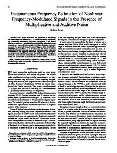
Fig. 1. (a) The AFS (b) The spectrogram of the fixed window length. The AFS shown in Fig. 1(a) resolved closely placed signal components whereas fixed window length spectrogram shown in Fig. 1(b) failed to do so.

Fig. 3. Step by step illustration of the component extraction procedure. (a) Exin solid line). (b) Extracted second component tracted first component ( in solid line). (

Fig. 2. (a) Time slice taken from the AFS. (b) Time slice taken from the fixed window spectrogram. Fig. 2(a) shows two distinct peaks corresponding to the signal components. Whereas, Fig. 2(b) has failed to resolve two signal components and we wrongly see just one peak.

Fig. 1 shows its TFDs, obtained by computing the fixed window length spectrogram and the AFS. Slices from the AFS and the fixed window length spectrogram for the time instant 2 are shown in the Fig. 2. The slice of the AFS shows the distinct resolved peaks for two different signal components. Whereas, the fixed length spectrogram wrongly shows one large peak as it failed resolve the close signal components. B. Signal Component Extraction The time-frequency separable signal components are extracted using the procedure presented in [9]. The key algorithm steps are listed below: 1. Initialize . 2. Find out , the location of maximum energy in the TFD. The IF of the th component at the time instant is computed to be . All points from to are assigned zero value. is a predetermined value. 3. Assign and . is the sampling frequency. The IF of the signal component for sub-regions and is computed by performing following steps: a) Find out the frequency having the maximum energy in the range to and in the range to . IF at instances and are computed to be (8)

b) Assign zero in the range to and to . c) Assign and . d) Repeat from step (a) till the boundary of the TFD is reached. 4. Increment ‘ ’ and repeat from step 2 till all the components have been extracted. The IF of each composing mono-component of the multicomponent signal is estimated by first computing the AFS using the method presented in II.A. Example: Fig. 3 shows the step by step illustration of the signal extraction procedure applied on the AFS computed in the previous subsection. III. EXPERIMENTAL RESULTS AND DISCUSSION A. Results In order to compare the IF estimation capability of the AFS with other TFDs, we consider the same multicomponent signal that was used in Section II. The multicomponent signal is analyzed using the modified B-distribution, WVD, spectrogram, AFS and multiview TFD based on the EMD (EMD-TFD) [10]. The IF is computed by applying the signal component extraction procedure presented in the Section II.B. The mean square error (MSE) is estimated by performing 100 simulations. Fig. 4 shows the results of the IF estimates. B. Discussion and Interpretation of Results The IF estimation capability of a TFD depends upon its’ ability to resolve closely placed signal components and reduce cross-terms. The spectrogram does not suffer from cross-term problem but fails to resolve closely placed components while the other smoothed versions of the WVD fail to suppress the cross-terms of such signals. The AFS overcomes the resolution limitation of the spectrogram by employing the adaptive window for each point in the TFD. Therefore, the MSE of IF estimates computed using the AFS is lower than the MSE of IF estimates obtained from other TFDs for SNR varying from dB to 16 dB as shown in Fig. 4; for example it is lower than

160


Fig. 4. (a) The plot of the MSE of the IF estimate of vs. SNR (b) The vs. SNR. The MSE of IF estimates plot of the MSE of the IF estimate of obtained using the AFS is lower than the MSE of IF estimates computed from all the other TFDs for all the noise levels; for example the MSE of the AFS is in lower than the MSE of the other multiview TFD described in [10] by scale for 10 dB SNR.

the MSE of the other multiview TFD described in [10] by in scale for 10 dB SNR. IV. CONCLUSION AND FUTURE WORK A novel approach to compute the instantaneous frequency (IF) of a multicomponent signal has been presented. This procedure defines a high resolution multiview time frequency distribution (TFD) which can be utilized to accurately compute the IF of closely placed signal components. The mean square error (MSE) of IF estimates computed using the AFS is lower than the MSE of IF estimates obtained from all the other TFDs for SNR varying from dB to 16 dB. The proposed IF estimation scheme requires additional information about the number of components that can be computed using the short term time-frequency Rényi entropy [16]. REFERENCES [1] B. Boashash, “Estimating and interpreting the IF of a signal. I. fundamentals,” Proc. IEEE, vol. 80, no. 4, pp. 520–538, Apr. 1992, DOI: 10.1109/5.135378.

[2] T. Qian, “Mono-components for decomposition of signals,” Math. Meth. Appl. Sci., vol. 29, pp. 1187–1198, 2006, DOI: 10.1002/mma.721. [3] B. Boashash, Time-Frequency Signal Analysis and Processing: A Comprehensive Reference. Amsterdam, The Netherlands: Elsevier, 2003. [4] Z. Yun, L. Shiping, L. Peng, and Z. Qiuping, “Instantaneous frequency measurement based on EMD and TVAR,” in 10th Int. Conf. Electronic Measurement & Instruments (ICEMI), 2011, vol. 3, pp. 303–306, Aug. 2011, DOI: 10.1109/ICEMI.2011.6037911. [5] T. Qian, L. Zhang, and H. Li, “Mono-components vs IMFS in signal decomposition,” Int. J. Wavelets, Multires. Inf. Process., vol. 6, no. 3, pp. 353–374, 2008, DOI: 10.1142/S0219691308002392. [6] V. Katkovnik and L. Stankovic, “IF estimation using the Wigner distribution with varying and data-driven window length,” IEEE Trans. Signal Process., vol. 46, no. 9, pp. 2315–2325, Sep. 1998, DOI: 10.1109/78.709514. [7] J. Lerga and V. Sucic, “Nonlinear IF estimation based on the pseudo WVD adapted using the improved sliding pair wise ICI rule,” IEEE Signal Process. Lett., vol. 16, no. 11, pp. 953–956, Nov. 2009, DOI: 10.1109/LSP.2009.2027651. [8] J. Lerga, V. Sucic, and B. Boashash, “An efficient algorithm for IF estimation of non-stationary multi-component signals in low SNR,” EURASIP J. Adv. Signal Process., p. 725189, Jan. 2011, 2011, DOI:10. 1155/2011/725189. [9] B. Barkat and K. Abed-Meraim, “Algorithms for blind components separation and extraction from the time-frequency distribution of their mixture,” EURASIP J. Appl. Signal Process., vol. 13, pp. 2025–2033, Jan. 2004, DOI: 10.1155/S1110865704404193. [10] N. J. Stevenson, M. Mesbah, and B. Boashash, “Multiple-view timefrequency distribution based on the empirical mode decomposition,” Signal Process., vol. 4, no. 4, pp. 446–456, Aug. 2010, DOI: 10.1049/ iet-spr.2009.0084. [11] H. Lee and Z. Z. Bien, “A variable bandwidth filter for estimation of instantaneous frequency and reconstruction of signals with timevarying spectral content,” IEEE Trans. Signal Process., vol. 59, no. 5, pp. 2052–2071, May 2011, DOI: 10.1109/TSP.2011.2113345. [12] R. G. Stockwell, L. Mansinha, and R. P. Lowe, “Localization of the complex spectrum: The S transform,” IEEE Trans. Signal Process., vol. 44, no. 4, pp. 998–1001, Apr. 1996, DOI: 10.1109/78.492555. [13] E. Sejdic, I. Djurovic, and J. Jiang, “A window width optimized S-transform,” EURASIP J. Adv. Signal Process., 2008, 2008. DOI:10.1155/2008/672941. [14] C. Capus and K. Brown, “Short-time fractional Fourier methods for the time frequency representation of chirp signals,” J. Acoust. Soc. Amer., vol. 113, no. 6, pp. 3253–3263, Jun. 2003, DOI: 10.1121/1.1570434. [15] L. Stankovic, T. Alieva, and M. J. Bastiaans, “Time-frequency signal analysis based on the windowed fractional Fourier transform,” Signal Process., vol. 83, no. 11, pp. 2459–2468, Aug. 2003, DOI: 10.1016/ S0165-1684(03)00197-X. [16] V. Sucic, N. Saulig, and B. Boashash, “Estimating the number of components of a multicomponent non stationary signal using the short-term time-frequency Rényi entropy,” EURASIP J. Adv. Signal Process., vol. 2011, p. 125, Dec. 2011, DOI: 10.1186/1687-6180-2011-125.