Estimation of Copula Models with Discrete Margins Michael S. Smith𝑎,★ & Mohamad A. Khaled𝑏 𝑎
Melbourne Business School, University of Melbourne 𝑏
University of Sydney October 31, 2010
★
Corresponding Author; address for correspondence: Professor Michael Smith, Melbourne Busi-
ness School, University of Melbourne, 200 Leicester Street, Carlton, VIC 3053, Australia. Email:
[email protected]
1
Estimation of Copula Models with Discrete Margins Abstract Estimation of copula models with discrete margins is known to be difficult beyond the bivariate case. We show how this can be achieved by augmenting the likelihood with uniform latent variables, and computing inference using the resulting augmented posterior. To evaluate this we propose two efficient Markov chain Monte Carlo sampling schemes. One generates the latent variables as a block using a Metropolis-Hasting step with a proposal that is close to its target distribution. Our method applies to all parametric copulas where the conditional copula functions can be evaluated, not just elliptical copulas as in previous Bayesian work. Moreover, the copula parameters can be estimated joint with any marginal parameters. We establish the effectiveness of the estimation method by modeling consumer behavior in online retail using Archimedean and Gaussian copulas. To demonstrate the potential in higher dimensions we estimate 16 dimensional D-vine copulas for a longitudinal model of usage of a bicycle path in the city of Melbourne, Australia. The estimates reveal an interesting serial dependence structure that can be represented in a parsimonious fashion using Bayesian selection of independence pair-copula components. Finally, we extend our results and method to the case where some margins are discrete and others continuous.
Key Words: Archimedian Copula; Bicycle Usage; Data Augmentation; Discrete Time Series; Markov chain Monte Carlo; D-vine; Online Retail.
1
Introduction
Copulas have proven a very successful way of modeling dependence in multivariate models. They are now used in a diverse range of applications, proving particularly popular in survival analysis (Clayton 1978; Oakes 1989), finance (Cherubini et al. 2004; McNeil, Frey and Embrechts 2005), econometrics (Cameron et al. 2004; Patton 2006) and actuarial science (Frees and Valdez 1998). In the vast majority of instances, parametric copula functions are employed for continuous data. In this case the copula parameters, and any marginal model parameters, can be readily estimated using maximum likelihood or other methods. However, in the case when the data are modeled as discrete, estimation by maximum likelihood is difficult beyond the bivariate case (Trivedi & Zimmer 2005). This has limited the use of copulas in fields where multivariate discrete data are common, such as marketing (Danaher & Smith 2010) and health economics (Cameron et al. 2004). We address this problem here by outlining how to compute likelihood based inference for parametric copula models with discrete margins, or when there is a mixture of discrete and continuous margins. We specify a joint distribution for the discrete random variables augmented with uniform latent variables. We show that the resulting margin in the discrete variables has the correct probability mass function of the copula model. The copula parameters, and any marginal model parameters, are estimated using the augmented posterior distribution evaluated using two Markov chain Monte Carlo (MCMC) sampling schemes. One is an extension of that suggested by Pitt, Chan and Kohn (2006), where the latents are generated one a time, to non-elliptical copulas. The other generates the latents as a block using a MetropolisHastings step with a proposal from which it is fast to generate, but is close to the target distribution. Different measures of dependence, including pairwise tail dependence, can be computed from the fitted copula. The Bayesian approach can be used in high dimensions, and for any copula where the conditional copula distribution function can be evaluated, which includes all popular parametric copulas employed currently. We also show how to extend the methodology to the case where some margins are discrete and others continuous. We demonstrate our approach using two examples. The first is a bivariate marketing
1
study of online consumer behavior at amazon.com. We show that the level of exposure to the website during a visit is positively related to both the amount spent and purchase incidence. In both cases the dependence is driven by positive lower tail dependence, rather than upper tail dependence. This is well captured by one and two parameter Archimedean copulas, but not a Gaussian copula with symmetric zero tail dependence. We show that ignoring the discrete nature of the data and treating the margins as continuous gives highly erroneous results, and should not be done. A new and flexible copula for higher dimensional data is the D-vine (Joe 1996; Bedford and Cooke 2002; Aas et al. 2009; Haff, Aas and Frigessi 2010), which is constructed from a sequence of bivariate ‘pair-copulas’. Our second example is a 16 dimensional longitudinal D-vine copula model for the number of bicycles travelling down a bike path in Melbourne, Australia. Each margin corresponds to the count of the number of bicycles that pass each hour. Smith et al. (2010) show that a D-vine copula model is well-motivated for the analysis of serial dependence in longitudinal data. The bike path is mainly used by commuters, and an interesting sparse dependence structure is uncovered. There is strong first order serial dependence throughout the day, along with positive dependence between the morning and late afternoon commuting periods. We evaluate the bivariate margin in the morning and late afternoon peak hours from D-vines with Gumbel and t pair-copulas, and find that the strong positive dependence is nonlinear. We show that choice of copula is important by comparing the ability of different copulas to forecast the evening peak count, given the morning peak. Pitt et al. (2006) propose a Bayesian method for the estimation of a Gaussian copula with discrete margins by augmentation with Gaussian latent variables. Their approach is shown to work in a 45 dimensional example in Danaher and Smith (2010) and is currently the only effective method for estimating high dimensional discrete-margined copulas. Our paper extends this approach to non-elliptical copula, provides the distributional theory for data augmentation, proposes new and more effective sampling schemes, and demonstrates the usefulness of the methodology in a number of contemporary applications where the dependence structure is too complex to be captured by elliptical copulas.
2
2
Copula Models for Discrete Data
2.1
Copula Function
The function 𝐶(𝑢1, ..., 𝑢𝑚 ) is called a copula function if it is a distribution function with each of its margins uniformly distributed on [0, 1]. That is, 𝐶(𝒖) = Pr(𝑈1 ≤ 𝑢1 , ..., 𝑈𝑚 ≤ 𝑢𝑚 ), with each 𝑈𝑗 , for 𝑗 = 1, . . . , 𝑚, uniformly distributed on [0, 1] and 𝒖 = (𝑢1, . . . , 𝑢𝑚 ). The density 𝑐(𝒖) = ∂𝐶(𝒖)/(∂𝒖) is called the copula density. Joe (1997) and Nelsen (2006) discuss a wide range of choices for 𝐶 and their properties. Following Sklar (1959) a joint distribution function 𝐹 with marginal distribution functions 𝐹1 , . . . , 𝐹𝑚 can be written as
𝐹 (𝒙) = 𝐶(𝐹1 (𝑥1 ), . . . , 𝐹𝑚 (𝑥𝑚 )) ,
(2.1)
with 𝒙 = (𝑥1 , . . . , 𝑥𝑚 ). When 𝐹1 , . . . , 𝐹𝑚 are strictly monotonically increasing, and therefore correspond to continuous margins, 𝐶 is known to be unique. However, when one or more marginal distribution is discrete, this is no longer the case; see Genest & Neˇslehov´a (2007) for a discussion. Nevertheless, the copula model in equation (2.1) remains a well-defined distribution function 𝐹 for any admissible copula function 𝐶. Moreover, in applied modeling 𝐶 is almost always picked from a parametric family, and 𝐹 defined in this manner; for example, see Cameron et al. (2004).
2.2
Augmented Distribution
Consider the case where 𝑿 = (𝑋1 , . . . , 𝑋𝑚 ) are all discrete and has distribution function 𝐹 at equation (2.1). Let 𝑏𝑗 = 𝐹𝑗 (𝑥𝑗 ), and 𝑎𝑗 = 𝐹𝑗 (𝑥− 𝑗 ) be the left hand limit of 𝐹𝑗 at 𝑥𝑗 , which is 𝑏𝑗 = 𝐹𝑗 (𝑥𝑗 − 1) in the case where 𝑋𝑗 is ordinal. Then, the probability mass function of 𝑿 can be expressed in closed form as 𝑓 (𝒙) = Pr(𝑋1 = 𝑥1 , . . . , 𝑋𝑚 = 𝑥𝑚 ) = Δ𝑏𝑎11 Δ𝑏𝑎22 ⋅ ⋅ ⋅ Δ𝑏𝑎𝑚𝑚 𝐶(𝒗) ,
3
(2.2)
where 𝒗 = (𝑣1 , . . . , 𝑣𝑚 ) and we employ the difference notation of Nelsen (2006; p.43): Δ𝑏𝑎𝑘𝑘 𝐶(𝑢1 , . . . , 𝑢𝑘−1, 𝑣𝑘 , 𝑢𝑘+1, . . . , 𝑢𝑚 ) = 𝐶(𝑢1 , . . . , 𝑢𝑘−1, 𝑏𝑘 , 𝑢𝑘+1, . . . , 𝑢𝑚 ) − 𝐶(𝑢1 , . . . , 𝑢𝑘−1, 𝑎𝑘 , 𝑢𝑘+1, . . . , 𝑢𝑚) . where 𝑣𝑘 is an index of differencing. For example, when 𝑚 = 3, 𝑓 (𝑥1 , 𝑥2 , 𝑥3 ) = Δ𝑏𝑎11 Δ𝑏𝑎22 Δ𝑏𝑎33 𝐶(𝑣1 , 𝑣2 , 𝑣3 ) = 𝐶(𝑏1 , 𝑏2 , 𝑏3 ) − 𝐶(𝑏1 , 𝑏2 , 𝑎3 ) − 𝐶(𝑏1 , 𝑎2 , 𝑏3 ) − 𝐶(𝑎1 , 𝑏2 , 𝑏3 ) +𝐶(𝑏1 , 𝑎2 , 𝑎3 ) + 𝐶(𝑎1 , 𝑏2 , 𝑎3 ) + 𝐶(𝑎1 , 𝑎2 , 𝑏3 ) − 𝐶(𝑎1 , 𝑎2 , 𝑎3 ) . In general, estimation of any copula parameters for 𝐶 using direct maximum likelihood estimation is difficult. First, there are 2𝑚 terms in the sum at equation (2.2), so that to compute the likelihood for 𝑛 observations involves 𝑛2𝑚 evaluations of 𝐶, which is prohibitive for larger values of 𝑚. Second, even in the case when 𝑚 = 3 or 𝑚 = 4, the likelihood can prove difficult to maximise for some datasets, particularly when the copula and marginal parameters are estimated jointly. We instead consider the joint distribution of (𝑿, 𝑼 ), with 𝑼 = (𝑈1 , . . . , 𝑈𝑚 ). To express this, first note that 𝐹𝑗 is a many-to-one function and 𝑋𝑗 ∣𝑈𝑗 is a degenerate distribution with density 𝑓 (𝑥𝑗 ∣𝑢𝑗 ) = ℐ(𝐹𝑗 (𝑥− 𝑗 ) ≤ 𝑢𝑗 < 𝐹𝑗 (𝑥𝑗 )). Here, the indicator function ℐ(𝐴) = 1 if 𝐴 is true, and zero otherwise. Then (𝑿, 𝑼 ) has mixed probability density
𝑓 (𝒙, 𝒖) = 𝑓 (𝒙∣𝒖)𝑐(𝒖) =
𝑚 ∏ 𝑗=1
where 𝑓 (𝒙∣𝒖) = Proposition 1
ℐ(𝐹𝑗 (𝑥− 𝑗 ) ≤ 𝑢𝑗 < 𝐹𝑗 (𝑥𝑗 ))𝑐(𝒖) ,
(2.3)
∏𝑚
𝑗=1 𝑓 (𝑥𝑗 ∣𝑢𝑗 ).
If (𝑿, 𝑼 ) has mixed probability density given by equation (2.3), then the marginal probability mass function of 𝑿 is given by equation (2.2). Proof : See Appendix.
4
2.3
Latent Variable Distributions
We show in Section 3 how to estimate any copula parameters using the likelihood augmented with latent variables distributed as 𝑼 . The computations are undertaken using Markov chain Monte Carlo (MCMC) algorithms. To develop these, the conditional distributions of the latent variables require evaluation. From equation (2.3) the density of 𝑼 ∣𝑿 is 𝑚
𝑐(𝒖) ∏ ℐ(𝑎𝑗 ≤ 𝑢𝑗 < 𝑏𝑗 ) . 𝑓 (𝒖∣𝒙) = 𝑓 (𝒙) 𝑗=1
(2.4)
However, for a subset of elements of 𝑼 the conditional distribution is more complex. Proposition 2 For 𝑗 = 1, . . . , 𝑚 − 1 the density of (𝑈1 , . . . , 𝑈𝑗 )∣𝑿 is 𝑓 (𝑢1 , . . . , 𝑢𝑗 ∣𝒙) =
𝑗 )∏ 𝑐(𝑢1 , . . . , 𝑢𝑗 ) ( 𝑏𝑗+1 Δ𝑎𝑗+1 ⋅ ⋅ ⋅ Δ𝑏𝑎𝑚 𝐶 (𝑣 , . . . , 𝑣 ∣𝑢 , . . . , 𝑢 ) ℐ(𝑎𝑘 ≤ 𝑢𝑘 < 𝑏𝑘 ) , 𝑗+1 𝑚 1 𝑗 𝑚 𝑗+1,...,𝑚∣1,...,𝑗 𝑓 (𝒙)
where 𝑐(𝑢1 , . . . , 𝑢𝑗 ) = 𝑈𝑗+1 , . . . 𝑈𝑚 ∣𝑈1 , . . . , 𝑈𝑗 .
𝑘=1
∫
𝑐(𝒖)d𝑢𝑗+1 . . . d𝑢𝑚 and 𝐶𝑗+1,...,𝑚∣1,...,𝑗 is the distribution function of
Proof : See Appendix. Here, we note that 𝑐(𝑢1 , . . . , 𝑢𝑗 ) is the marginal copula density with support on [0, 1]𝑗 , while Proposition 2 shows that 𝑓 (𝑢1 , . . . , 𝑢𝑗 ∣𝒙) has support on [𝑎1 , 𝑏1 )×⋅ ⋅ ⋅×[𝑎𝑗 , 𝑏𝑗 ). The density has 2𝑚−𝑗 terms, and when 𝑗 = 𝑚, the density at equation (2.4) results. Throughout the paper if 𝐼1 ⊂ {1, . . . , 𝑚}, 𝐼2 ⊂ {1, . . . , 𝑚} and 𝐼1 ∩𝐼2 = ∅, then we denote the conditional distribution and density functions of 𝑈𝑗∈𝐼1 ∣𝑈𝑗∈𝐼2 as 𝐶𝐼1 ∣𝐼2 and 𝑐𝐼1 ∣𝐼2 , respectively. The corollary below is used in developing MCMC sampling algorithms. Corollary 1 For 𝑗 = 2, . . . , 𝑚 the conditional distribution of 𝑈𝑗 ∣𝑈1 , . . . , 𝑈𝑗−1 , 𝑿 is 𝑓 (𝑢𝑗 ∣𝑢1 , . . . , 𝑢𝑗−1, 𝒙) = 𝑐𝑗∣1,...,𝑗−1 (𝑢𝑗 ∣𝑢1, . . . , 𝑢𝑗−1)ℐ(𝑎𝑗 ≤ 𝑢𝑗 < 𝑏𝑗 )𝒦𝑗 (𝑢1 , . . . , 𝑢𝑗 ), ,
5
( ) where 𝒦𝑚 (𝒖) = 1/ Δ𝑏𝑎𝑚𝑚 𝐶𝑚∣1,...,𝑚−1 (𝑣𝑚 ∣𝑢1 . . . , 𝑢𝑚−1 ) , and for 𝑗 = 2, . . . , 𝑚 − 1: 𝑏
𝒦𝑗 (𝑢1 , . . . , 𝑢𝑗 ) =
𝑏𝑚 Δ𝑎𝑗+1 𝑗+1 ⋅ ⋅ ⋅ Δ𝑎𝑚 𝐶𝑗+1,...,𝑚∣1,...,𝑗 (𝑣𝑗+1 , . . . , 𝑣𝑚 ∣𝑢1 , . . . , 𝑢𝑗 ) 𝑏
Δ𝑎𝑗𝑗 ⋅ ⋅ ⋅ Δ𝑏𝑎𝑚𝑚 𝐶𝑗,...,𝑚∣1,...,𝑗−1(𝑣𝑗 , . . . , 𝑣𝑚 ∣𝑢1 , . . . , 𝑢𝑗−1)
.
Proof : Follows immediately from Proposition 2 by considering 𝑓 (𝑢𝑗 ∣𝑢1, . . . , 𝑢𝑗−1, 𝒙) = 𝑓 (𝑢1 , . . . , 𝑢𝑗 ∣𝒙)/𝑓 (𝑢1, . . . , 𝑢𝑗−1∣𝒙).
3
Estimation & Inference
3.1
Augmented Likelihood and Priors
In applied analysis, a copula function is usually selected from a parametric family and parametric models are often used for the margins. If 𝜃𝑗 are the parameters of margin 𝑗, and 𝜙 are the copula parameters, we denote the marginal distribution functions as 𝐹𝑗 (𝑥𝑗 ; 𝜃𝑗 ), copula function as 𝐶(𝒖; 𝜙) and copula density as 𝑐(𝒖; 𝜙). Consider an independent sample of 𝑛 observations, each with distribution function given at equation (2.1). Throughout the rest of this section we denote each observation as 𝒙𝑖 = (𝑥𝑖,1 , . . . , 𝑥𝑖,𝑚 ), and 𝒙 = {𝒙1 , . . . , 𝒙𝑛 }. To estimate Θ = {𝜃1 , . . . , 𝜃𝑚 } and 𝜙 we introduce latent variables 𝒖𝑖 = (𝑢𝑖,1 , . . . , 𝑢𝑖,𝑚 ), for 𝑖 = 1, . . . , 𝑛, with (𝒙𝑖 , 𝒖𝑖 ) having joint density at equation (2.3). The augmented likelihood is 𝑓 (𝒖, 𝒙∣Θ, 𝜙) =
𝑛 ∏ 𝑖=1
𝑓 (𝒙𝑖 , 𝒖𝑖 ∣Θ, 𝜙) =
𝑛 ∏ 𝑖=1
𝑐(𝒖𝑖 ; 𝜙)
𝑚 ∏ 𝑗=1
ℐ(𝑎𝑖,𝑗 ≤ 𝑢𝑖,𝑗 < 𝑏𝑖,𝑗 ) ,
(3.1)
where 𝑎𝑖,𝑗 = 𝐹𝑗 (𝑥− 𝑖,𝑗 ; 𝜃𝑗 ), 𝑏𝑖,𝑗 = 𝐹𝑗 (𝑥𝑖,𝑗 ; 𝜃𝑗 ) and 𝒖 = {𝒖1 , . . . , 𝒖𝑛 }. Throughout the rest of this section it is important to remember that 𝑎𝑖,𝑗 and 𝑏𝑖,𝑗 are functions of 𝜃𝑗 and 𝑥𝑖,𝑗 . In some problems, such as in multivariate financial time series models (Patton 2006; Jondeau & Rockinger 2006), the marginal distributions vary over observation.
In this
case the marginal distribution functions are denoted as 𝐹𝑖,𝑗 , with 𝑎𝑖,𝑗 = 𝐹𝑖,𝑗 (𝑥− 𝑖,𝑗 ; 𝜃𝑗 ) and 𝑏𝑖,𝑗 = 𝐹𝑖,𝑗 (𝑥𝑖,𝑗 ; 𝜃𝑗 ). In other problems the empirical distribution function is employed for the margins (Oakes 1994; Genest et al. 1995; Shih & Louis 1995). 6
We assume the prior density 𝜋(𝒖, Θ, 𝜙) = 𝑐(𝒖; 𝜙)𝜋(𝜙)
∏𝑚
𝑗=1 𝜋(𝜃𝑗 ),
where 𝜋(𝜙) is specific
to the choice of copula, and 𝜋(𝜃𝑗 ) is specific to any marginal model chosen.
3.2
Posterior of Copula Parameters
In our sampling schemes, we generate the copula parameters 𝜙 conditional upon 𝒖. The posterior 𝑓 (𝜙∣𝒖, Θ, 𝒙) = 𝑓 (𝜙∣𝒖) ∝
𝑛 ∏
𝑐(𝒖𝑖 ; 𝜙)𝜋(𝜙) ,
𝑖=1
so that the approach depends upon the type of copula 𝐶, and the prior 𝜋(𝜙). For an elliptical copula this involves generation of a correlation matrix. Pitt et al. (2006) show how to do this for a covariance selection prior, while Danaher & Smith (2010) show how to do it with a prior on a Cholesky factor based decomposition. Other priors, such as that in Daniels & Pourahmadi (2009) or Barnard, McCulloch & Meng (2000), can also be employed here. For many other copulas the parameters can be generated one parameter at a time using a Metropolis-Hastings (MH) step with a random walk (Robert & Cassella 2004, pp.287-291) or other proposal. In our empirical work we show that this works well for several Archimedean and D-vine copulas.
3.3
Posterior of Latent Variables
The posterior 𝑓 (𝒖∣𝜙, Θ, 𝒙) = cated distribution.
∏𝑛
𝑖=1
𝑓 (𝒖𝑖 ∣𝜙, Θ, 𝒙𝑖), where 𝒖𝑖 ∣𝜙, Θ, 𝒙𝑖 has a multivariate trun-
We generate an iterate from 𝑓 (𝒖𝑖 ∣𝜙, Θ, 𝒙𝑖 ) using proposal densities
𝑔𝑗 (𝑢𝑖,𝑗 ), for 𝑗 = 1, . . . , 𝑚. These are proportional to 𝑐𝑗∣1,...,𝑗−1 (𝑢𝑖,𝑗 ∣𝑢𝑖,1 , . . . , 𝑢𝑖,𝑗−1; 𝜙), and truncated to [𝑎𝑖,𝑗 , 𝑏𝑖,𝑗 ), so that
𝑔𝑗 (𝑢𝑖,𝑗 ) =
𝑐𝑗∣1,...,𝑗−1(𝑢𝑖,𝑗 ∣𝑢𝑖,1, . . . , 𝑢𝑖,𝑗−1; 𝜙)ℐ(𝑎𝑖,𝑗 ≤ 𝑢𝑖,𝑗 < 𝑏𝑖,𝑗 ) . 𝐶𝑗∣1,...,𝑗−1 (𝑏𝑖,𝑗 ∣𝑢𝑖,1, . . . , 𝑢𝑖,𝑗−1; 𝜙) − 𝐶𝑗∣1,...,𝑗−1 (𝑎𝑖,𝑗 ∣𝑢𝑖,1, . . . , 𝑢𝑖,𝑗−1; 𝜙)
(3.2)
When 𝑗 = 1, 𝑔1 (𝑢𝑖,1) = ℐ(𝑎𝑖,1 ≤ 𝑢𝑖,1 < 𝑏𝑖,1 )/(𝑏𝑖,1 − 𝑎𝑖,1 ), and when 𝑗 = 𝑚, from Corollary 1, 𝑔𝑚 (𝑢𝑖,𝑚 ) = 𝑓 (𝑢𝑖,𝑚∣𝑢𝑖,1 , . . . , 𝑢𝑖,𝑚−1, 𝒙𝑖 ). For 𝑗 < 𝑚, 𝑔𝑗 (𝑢𝑖,𝑗 ) is close to 𝑓 (𝑢𝑖,𝑗 ∣𝑢𝑖,1, . . . , 𝑢𝑖,𝑗−1, 𝒙, 𝜙, Θ), with the difference being determined by the normalizing constant of 𝑔𝑗 and the term 𝒦𝑗 (𝑢𝑖,1 , . . . , 𝑢𝑖,𝑗 ) 7
defined in Corollary 1. However, it is much faster to generate from 𝑔𝑗 as long as the conditional copula distribution is available. We consider two different MH algorithms. Method 1: For 𝑗 = 1, . . . , 𝑚 sequentially generate 𝑢new 𝑖,𝑗 from 𝑔𝑗 , and separately accept each value over the previous value 𝑢old 𝑖,𝑗 with probability min(1, 𝛼𝑖,𝑗 ), where 𝛼𝑖,𝑚 = 1 and for 𝑗 < 𝑚,
𝛼𝑖,𝑗 =
𝑏
𝑏
𝑏
𝑏
𝑖,𝑚 new Δ𝑎𝑖,𝑗+1 𝑖,𝑗+1 ⋅ ⋅ ⋅ Δ𝑎𝑖,𝑚 𝐶𝑗+1,...,𝑚∣1,...,𝑗 (𝑣𝑗+1 , . . . , 𝑣𝑚 ∣𝑢𝑖,1 , . . . , 𝑢𝑖,𝑗−1 , 𝑢𝑖,𝑗 ; 𝜙) 𝑖,𝑚 old Δ𝑎𝑖,𝑗+1 𝑖,𝑗+1 ⋅ ⋅ ⋅ Δ𝑎𝑖,𝑚 𝐶𝑗+1,...,𝑚∣1,...,𝑗 (𝑣𝑗+1 , . . . , 𝑣𝑚 ∣𝑢𝑖,1 , . . . , 𝑢𝑖,𝑗−1 , 𝑢𝑖,𝑗 ; 𝜙)
.
Method 2: For 𝑗 = 1, . . . , 𝑚, sequentially generate 𝑢new 𝑖,𝑗 from 𝑔𝑗 , then accept the block new old old old 𝒖new = (𝑢new 𝑖 𝑖,1 , . . . , 𝑢𝑖,𝑚 ) over the previous values 𝒖𝑖 = (𝑢𝑖,1 , . . . , 𝑢𝑖,𝑚 ) with probability
min(1, 𝛼𝑖 ), where
𝛼𝑖 =
𝑚 new new new ∏ 𝐶𝑗∣1,...,𝑗−1(𝑏𝑖,𝑗 ∣𝑢new 𝑖,1 , . . . , 𝑢𝑖,𝑗−1 ; 𝜙) − 𝐶𝑗∣1,...,𝑗−1 (𝑎𝑖,𝑗 ∣𝑢𝑖,1 , . . . , 𝑢𝑖,𝑗−1 ; 𝜙) 𝑗=2
old old old 𝐶𝑗∣1,...,𝑗−1 (𝑏𝑖,𝑗 ∣𝑢old 𝑖,1 , . . . , 𝑢𝑖,𝑗−1 ; 𝜙) − 𝐶𝑗∣1,...,𝑗−1 (𝑎𝑖,𝑗 ∣𝑢𝑖,1 , . . . , 𝑢𝑖,𝑗−1; 𝜙)
.
Both 𝛼𝑖,𝑗 and 𝛼𝑖 above are derived using Corollary 1. Both methods provide an iterate from 𝑓 (𝒖𝑖 ∣𝜙, Θ, 𝒙𝑖 ), but Method 2 is computationally viable for higher values of 𝑚, whereas Method 1 is not. Note that as (𝐹𝑗 (𝑥; 𝜃𝑗 ) − 𝐹𝑗 (𝑥− ; 𝜃𝑗 )) → 0 for all 𝑗 (ie. the marginal old distributions get closer to being continuous) then 𝑢new 𝑖,𝑗 → 𝑢𝑖,𝑗 , so that 𝛼𝑖 → 1 and 𝛼𝑖,𝑗 → 1. ∏ In this sense, 𝑔(𝒖𝑖 ) = 𝑚 𝑗=1 𝑔𝑗 (𝑢𝑖,𝑗 ) is close to 𝑓 (𝒖𝑖 ∣𝜙, Θ, 𝒙𝑖 ), and we show in our empirical
work that even when modeling highly discrete data, Method 2 provides adequate acceptance rates.
3.4
Sampling Schemes
We denote 𝒖(𝑗) = {𝑢1,𝑗 , . . . , 𝑢𝑛,𝑗 } and 𝒙(𝑗) = {𝑥1,𝑗 , . . . , 𝑥𝑛,𝑗 }, and propose two sampling schemes to estimate 𝜙 and Θ jointly. Sampling Scheme 1 (SS1) (1) Generate from 𝑓 (Θ∣𝜙, 𝒙) (2) Generate from 𝑓 (𝒖∣Θ, 𝜙, 𝒙)
8
(3) Generate from 𝑓 (𝜙∣𝒖) Steps (1) and (2) together are equivalent to generating from 𝑓 (Θ, 𝒖∣𝜙, 𝒙) as a block, so that SS1 is likely to exhibit strong convergence and mixing. However, in Step (1)
𝑓 (Θ∣𝜙, 𝒙) ∝ 𝑓 (𝒙∣Θ, 𝜙)
𝑚 ∏
𝑛 ∏
𝜋(𝜃𝑗 ) =
𝑗=1
𝑖=1
Δ𝑏𝑎𝑖,1 𝑖,1
. . . Δ𝑏𝑎𝑖,𝑚 𝐶(𝒗; 𝜙) 𝑖,𝑚
𝑚 ∏
𝜋(𝜃𝑗 ) ,
(3.3)
𝑗=1
which requires computation of the likelihood 𝑓 (𝒙∣Θ, 𝜙). We generate Θ using MH with ∏ proposal density 𝑞(Θ) = 𝑚 𝑗=1 𝑞𝑗 (𝜃𝑗 ). We follow Chib & Greenberg (1998), Pitt et al. (2006)
and others and use a multivariate t density for 𝑞𝑗 with 𝜈 = 7 degrees of freedom. The proposal is centred around the estimate of 𝜃𝑗 obtained by two or three Newton-Raphson
steps starting from the marginal model estimate, and with scale equal to the negative of the inverse of the information matrix. We note that in problems where Θ has a large number of elements, it might prove attractive to partition Θ and generate from the resulting margins of 𝑓 (Θ∣𝜙, 𝒙). For Step (2) we generate 𝒖𝑖 using Method 2 outlined in Section 3.3. In the second sampling scheme we generate (𝜃𝑗 , 𝒖(𝑗) ) as a pair from the density
𝑓 (𝜃𝑗 , 𝒖(𝑗) ∣𝜃𝑘∕=𝑗 , 𝜙, 𝒖(𝑘∕=𝑗), 𝒙) = 𝑓 (𝜃𝑗 ∣𝜃𝑘∕=𝑗 , 𝜙, 𝒖(𝑘∕=𝑗), 𝒙)𝑓 (𝒖(𝑗) ∣Θ, 𝜙, 𝒖(𝑘∕=𝑗), 𝒙) , by first generating 𝜃𝑗 with 𝒖(𝑗) integrated out, and then 𝒖(𝑗) conditional upon 𝜃𝑗 . The sampling scheme we adopt is therefore: Sampling Scheme 2 (SS2) (1) For 𝑗 = 1, . . . , 𝑚: (1a) Generate from 𝑓 (𝜃𝑗 ∣𝜃𝑘∕=𝑗 , 𝜙, 𝒖(𝑘∕=𝑗), 𝒙) (1b) Generate from 𝑓 (𝒖(𝑗) ∣Θ, 𝜙, 𝒖(𝑘∕=𝑗), 𝒙) (2) Generate from 𝑓 (𝜙∣𝒖) A similar sampler was proposed by Pitt et al. (2006) for the specific case of a Gaussian copula, and SS2 is the extension to other copula models. In Step (1a) of SS2 we use a MH
9
step with proposal 𝑞𝑗 as in SS1, while the conditional posterior of 𝜃𝑗 is ∫
𝑓 (𝜃𝑗 ∣𝜃𝑘∕=𝑗 , 𝜙, 𝒖(𝑘∕=𝑗), 𝒙) ∝ 𝑓 (𝒙∣Θ, 𝜙, 𝒖(𝑘∕=𝑗))𝜋(𝜃𝑗 ) ∝ 𝑓 (𝒙, 𝒖∣Θ, 𝜙)d𝒖(𝑗) 𝜋(𝜃𝑗 ) } 𝑛 {∫ ∏ 𝑓 (𝒙𝑖 , 𝒖𝑖 ∣Θ, 𝜙)d𝑢𝑖,𝑗 𝜋(𝜃𝑗 ) , = 𝑖=1
so that from the augmented likelihood in equation (3.1):
𝑓 (𝜃𝑗 ∣𝜃𝑘∕=𝑗 , 𝜙, 𝒖(𝑘∕=𝑗), 𝒙) ∝ ∝
{∫ 𝑚 𝑛 ∏ ∏
𝑖=1 {∫ 𝑘=1 𝑛 𝑏𝑖,𝑗 ∏
{ℐ(𝑎𝑖,𝑘 ≤ 𝑢𝑖,𝑘 < 𝑏𝑖,𝑘 )} 𝑐(𝒖𝑖 ; 𝜙)d𝑢𝑖,𝑗
𝑐(𝒖𝑖 ; 𝜙)d𝑢𝑖,𝑗
𝑖=1
𝑎𝑖,𝑗
}
}
𝜋(𝜃𝑗 )
𝜋(𝜃𝑗 ) .
This is a very general expression for any copula. To evaluate the integral it requires the computation of the distribution function 𝐶𝑗∣𝑘∕=𝑗 of the conditional copula: 𝑛 ∏ { } 𝐶𝑗∣𝑘∕=𝑗 (𝑏𝑖,𝑗 ∣𝑢𝑖,𝑘∕=𝑗 ; 𝜙) − 𝐶𝑗∣𝑘∕=𝑗 (𝑎𝑖,𝑗 ∣𝑢𝑖,𝑘∕=𝑗 ; 𝜙) 𝜋(𝜃𝑗 ) . 𝑓 (𝜃𝑗 ∣𝜃𝑘∕=𝑗 , 𝜙, 𝒖(𝑘∕=𝑗), 𝒙) ∝ 𝑖=1
The conditional copula functions above can either be computed in closed form, or numerically, for a wide range of copulas. In Step (1b)
𝑓 (𝒖(𝑗) ∣Θ, 𝜙, 𝒖(𝑘∕=𝑗), 𝒙) ∝ 𝑓 (𝒙∣Θ, 𝒖)𝑓 (𝒖(𝑗)∣𝜙, 𝒖(𝑘∕=𝑗)) 𝑛 𝑛 ∏ ∏ ∝ ℐ(𝑎𝑖,𝑗 ≤ 𝑢𝑖,𝑗 < 𝑏𝑖,𝑗 )𝑐(𝒖𝑖 ; 𝜙) ∝ ℐ(𝑎𝑖,𝑗 ≤ 𝑢𝑖,𝑗 < 𝑏𝑖,𝑗 )𝑐𝑗∣𝑘∕=𝑗 (𝑢𝑖,𝑗 ∣𝑢𝑖,𝑘∕=𝑗 ; 𝜙) . 𝑖=1
𝑖=1
Therefore, the latents 𝑢𝑖,𝑗 are generated from the conditional densities 𝑐𝑗∣𝑘∕=𝑗 constrained to [𝑎𝑖,𝑗 , 𝑏𝑖,𝑗 ), and an iterate for 𝒖(𝑗) obtained. Last, we make some additional comments regarding the two samplers. First, in SS1 Θ is generated with 𝒖 integrated out. While it is tempting to generate conditional upon 𝒖, note that
𝑓 (Θ∣𝜙, 𝒖, 𝒙) ∝ 𝑓 (𝒙∣Θ, 𝒖)𝜋(Θ) =
𝑚 ∏ 𝑛 ∏ 𝑗=1 𝑖=1
𝐼(𝑎𝑖,𝑗 ≤ 𝑢𝑖,𝑗 < 𝑏𝑖,𝑗 )𝜋(𝜃𝑗 ) =
10
𝑚 ∏ 𝑗=1
𝑓 (𝜃𝑗 ∣𝒖(𝑗) , 𝒙(𝑗)) .
This suggests there is likely to be very high dependence between the marginal parameters 𝜃𝑗 and 𝒖𝑗 ; a similar observation is made by Pitt et al. (2006). Second, for large values of 𝑚 SS1 is computationally impractical and SS2 preferred. However, for values of 𝑚 less than about 8, SS1 is our preferred sampler. Third, in much empirical work copula parameters are estimated conditional upon the margins. In this case SS1 is preferred to SS2 for all values of 𝑚 because 𝒖 is generated as a block. Fourth, we bound 𝑎𝑖,𝑗 and 𝑏𝑖,𝑗 to (𝜖, 1 − 𝜖), with 𝜖 = 0.0001 to ensure numerical stability.
3.5
Bayesian Estimates
After convergence, 𝐾 iterates {𝒖[𝑘], Θ[𝑘] , 𝜙[𝑘]; 𝑘 = 1 . . . , 𝐾} are collected from 𝑓 (𝒖, Θ, 𝜙∣𝒙), from which Monte Carlo estimates of the posterior means of parameters are computed and used as point estimates, along with posterior probability intervals. There are a number of popular pairwise dependence measures for non-Gaussian data, with a comprehensive summary given in Nelsen (2006; Chapter 5). Genest & Neˇslehov´a (2007) discuss the difficulties of computing dependence measures when one or more of the margins is discrete; see also Denuit & Lambert (2005). Problems arise when the copula function is not unique and when nonparametric measures are computed, neither of which is the case when computing inference from the augmented distribution at equation (2.3). We employ Spearman’s pairwise correlation 𝜌𝑖,𝑗 (𝜙) = 12𝐸(𝑈𝑖 𝑈𝑗 ) − 3 for margins 𝑖 and 𝑗, where 𝑼 has distribution function 𝐶(𝒖; 𝜙). We also employ Kendall’s tau 𝜏𝑖,𝑗 (𝜙) and the upper and lower tail dependence measures 𝜆𝑈𝑖,𝑗 (𝜙) = lim𝛼↑1 Pr(𝑈𝑖 > 𝛼∣𝑈𝑗 > 𝛼) and 𝜆𝐿𝑖,𝑗 (𝜙) = lim𝛼↓0 Pr(𝑈𝑖 < 𝛼∣𝑈𝑗 < 𝛼). To estimate these based on the fitted copula we compute their expectations with respect to the posterior distribution of the copula parameters 𝑓 (𝜙∣𝒙). For example, the ∫ estimate of the Spearman correlation is 𝐸(𝜌𝑖,𝑗 ) = 𝜌𝑖,𝑗 (𝜙)𝑓 (𝜙∣𝒙)d𝜙. For some copulas, such
as elliptical and many Archimedian copulas, the dependence measures can be expressed as a closed form function of 𝜙, and the expectations approximated with histogram estimates over the Monte Carlo iterates {𝜙[𝑘]; 𝑘 = 1, . . . , 𝐾}. However, closed form expressions are not
readily available for all copulas, including the vine copulas. In these circumstances, we can
11
still estimate the marginal pairwise Spearman’s correlation accurately by generating iterates 𝒖[𝑘] ∼ 𝐶(𝒖; 𝜙[𝑘]) from the copula at the end of each sweep of the sampling scheme, and then ∑𝐾 [𝑘] [𝑘] computing 𝐸(𝜌𝑖,𝑗 ) ≈ 12 𝑘=1 𝑢𝑖 𝑢𝑗 − 3. 𝐾
4
Online Retail at Amazon.com
Danaher and Smith (2010) show that marketing is an area where copula models with discrete margins have strong potential. To establish the effectiveness of our methodology we first consider two bivariate copula models of consumer behavior at amazon.com, the world’s largest online retailer. Because the models are bivariate the Bayesian estimates can be compared with those obtained by maximum likelihood. The data employed were collected by ComScore Inc., and made available by subscription via the Wharton Data Research Service. We analyze a randomly selected sample of 𝑛 = 10, 000 visits to amazon.com by US households during 2007. We consider the number of unique page views (𝑃 ∈ {0, 1, . . .}) and the sales amount (𝑆 ≥ 0) during a visit. Marketing studies treat 𝑃 as a measure of consumer exposure to a website, and the objective is to measure the level and form of dependence between this and both 𝑆 and purchase incidence. Website designers hope to observe positive dependence because they try to increase sales by making sites more ‘sticky’ for online visitors; see Danaher (2007) for a discussion. Table 2 provides a contingency table of the aggregated data. Most visits to amazon.com (92.3%) do not result in a sale, so that 𝑆 is highly zero-inflated. In our first model we treat the margins as fully ordinal-valued and employ empirical distributions for the margins of both 𝑆 and 𝑃 . Dependence is captured using Clayton (Clayton 1978), BB7 (Joe 1997; p.153) and Gaussian copulas, which have closed form expressions for the copula densities, distribution functions, and conditional distribution functions; see Table 1. The Clayton copula is a single parameter copula with 𝜆𝑈 = 0, the BB7 is a two parameter copula with asymmetric non-zero tail dependence, unlike the Gaussian copula where 𝜆𝑈 = 𝜆𝐿 = 0. The approach where the margins are estimated in a nonparametric manner, and any dependence captured using a parametric copula estimated in a second step, is widely advocated; see 12
Clayton (1978) for an early example. A second copula model employs a Bernoulli margin for purchase incidence and a negative binomial margin for 𝑃 (truncated so that 𝑃 > 0), where the latter is a widely used to model exposure counts (Danaher & Smith, 2010). Dependence is again captured using Clayton, BB7 and Gaussian copulas, and in this second model we jointly estimate the parameters of the marginal models and copulas. —–Tables 1 and 3—– Table 3 provides estimates of the copula and dependence parameters for both models. For comparison we also report the maximum likelihood estimates (MLEs), which can be calculated here because the copula is bivariate, and also the pseudo-maximum likelihood estimates (PMLE) obtained treating the data as continuous. Because the MLE is the posterior mode under flat priors, the Bayesian estimate and MLE are similar, with minor differences due to any asymmetry in the posterior distribution 𝑓 (𝜙∣𝒙). The PMLE dramatically understates the level of dependence, showing that it is essential to account for discreteness in the data to obtain accurate dependence measures. ˆ 𝑈 is close The level and form of dependence in both models is similar. For the BB7 copula 𝜆 ˆ 𝐿 = 0.86 and 0.87, which is almost identical to that obtained using the Clayton to zero and 𝜆 copula, suggesting that the restriction 𝜆𝑈 = 0 is not unreasonable. Highly asymmetric tail dependence suggests that an elliptical copula will fit the dependence structure poorly, with 𝜏ˆ = 0.43 and 0.44 for the Gaussian copula, which is markedly lower than 𝜏ˆ = 0.70 and 0.71 for both Archimedean copulas. From the copula model of (𝑆, 𝑃 ) we also compute estimates of 𝐸[𝑆∣𝑃 = 𝑝] = 𝑠, 𝑃 = 𝑝)/Pr(𝑃 = 𝑝), where
∑
𝑠
𝑠Pr(𝑆 =
Pr(𝑆 = 𝑠, 𝑃 = 𝑝) = 𝐶(𝐹𝑆 (𝑠), 𝐹𝑃 (𝑝); 𝜙) − 𝐶(𝐹𝑆 (𝑠), 𝐹𝑃 (𝑝 − 1); 𝜙) +𝐶(𝐹𝑆 (𝑠 − 1), 𝐹𝑃 (𝑝 − 1); 𝜙) − 𝐶(𝐹𝑆 (𝑠 − 1), 𝐹𝑃 (𝑝); 𝜙) , evaluated at the posterior mean 𝜙ˆ = 𝐸(𝜙∣𝒙). The summation is over the domain of 𝑆, but we approximate this over the unique observed values. Figure 1 plots the conditional expectation for values of 𝑃 between the 2.5th and 97.5th percentiles. For the Archimedean 13
copulas the expected spend in a visit increases as website exposure increases, although at a marginally decreasing rate; the almost linear relationship for the Gaussian copula reflects its more limited dependence structure. For the copula model of 𝑃 and purchase incidence, the estimates of the marginal parameters (unreported) show that joint estimation with the copula parameters has very little impact on the point estimates, something that is often observed empirically. Even though both models feature highly discrete margins, for the Gaussian, Clayton and BB7 copulas the proposal 𝑔 has mean acceptance rates of 72%, 43% and 40% when estimating the first model, and 71%, 48% and 48% when estimating the second. The schemes mix adequately as measured by simulation inefficiency factors (SIFs); see Kim et al (1998) for a discussion of this popular metric. When computed for the parameters in both models using the first 100 autocorrelation coefficients these vary from 5.5 to 134. The largest SIF corresponds to 𝜙2 for the BB7 copula, and SIFs for other parameters are considerably lower.
—–Figure 1 about here—–
5
D-Vine Copula with Discrete Margins
Vine copula functions 𝐶 are constructed from a sequence of simpler bivariate copula called ‘pair-copula’; see Kurowicka & Cooke (2006) and Haff et al. (2010) for overviews. However, to date they have been employed exclusively for the analysis of continuous data. We consider a D-vine copula, which is well-motivated as a model for longitudinal data, although the approach is equally applicable to other vines. Following Smith et al. (2010) we also extend our Bayesian method to allow for the selection of independence pair-copula components.
5.1
D-vine copula
We outline D-vines here in the context of longitudinal data, where 𝑿 in Section 2 has elements ordered in time and distribution function at equation (2.1), but refer the reader to Aas et al. (2009) and Smith et al. (2010) for detailed discussions. A parameteric D-vine 14
has a copula density which is the product of 𝑚(𝑚 − 1)/2 bivariate copula densities 𝑐𝑡,𝑗 , for 𝑡 = 2, . . . , 𝑚 and 𝑗 < 𝑡, with
𝑐(𝒖; 𝜙) =
𝑚 ∏ 𝑡=2
𝑐𝑡∣1,...,𝑡−1 (𝑢𝑡 ∣𝑢1 , . . . , 𝑢𝑡−1 ; 𝜙) =
𝑚 ∏ 𝑡−1 ∏
𝑐𝑡,𝑗 (𝑢𝑡∣𝑗+1, 𝑢𝑗∣𝑡−1; 𝜙𝑡,𝑗 ) ,
(5.1)
𝑡=2 𝑗=1
where 𝒖 = (𝑢1 , . . . , 𝑢𝑚 ). Each bivariate copula is called a ‘pair-copula’ and has copula parameters 𝜙𝑡,𝑗 . The parameters of the D-vine copula are the collection of all the paircopula parameters, so that 𝜙 = {𝜙𝑡,𝑠 ; 𝑡 = 2, . . . , 𝑚, 𝑗 < 𝑡}. The values 𝑢𝑡∣𝑗 = 𝐶𝑡∣𝑗,...,𝑡−1 (𝑢𝑡 ∣𝑢𝑡−1 , . . . , 𝑢𝑗 ; 𝜙) , 𝑢𝑗∣𝑡 = 𝐶𝑗∣𝑗+1,...,𝑡 (𝑢𝑗 ∣𝑢𝑡, . . . , 𝑢𝑗+1; 𝜙) , are computed through a recursive algorithm which employs the functions
ℎ𝑡,𝑗 (𝑣1 ∣𝑣2 ; 𝜙𝑡,𝑗 ) = where 𝐶𝑡,𝑗 (𝑢1 , 𝑢2 ; 𝜙𝑡,𝑗 ) =
∫ 𝑢1 ∫ 𝑢2 0
0
∂ 𝐶𝑡,𝑗 (𝑣1 , 𝑣2 ; 𝜙𝑡,𝑗 ) , ∂𝑣2
𝑐𝑡,𝑗 (𝑣1 , 𝑣2 ; 𝜙𝑡,𝑗 )d𝑣1 d𝑣2 . That is, ℎ𝑡,𝑗 is the conditional distri-
bution function of pair-copula 𝐶𝑡,𝑗 , which is given in closed form in Table 1 for the bivariate copula employed in this paper. The algorithm to compute the arguments of the pair-copulas in equation (5.1) is given below. Algorithm A (Evaluation of Arguments of Pair-Copulas) (1) For 𝑡 = 1, . . . , 𝑚 define 𝑢𝑡∣𝑡 = 𝑢𝑡 (2) For 𝑘 = 1, . . . , 𝑚 − 1 and 𝑖 = 𝑘 + 1, . . . , 𝑚 compute: Backwards Step: 𝑢𝑖∣𝑖−𝑘 = ℎ𝑖,𝑖−𝑘 (𝑢𝑖∣𝑖−𝑘+1∣𝑢𝑖−𝑘∣𝑖−1; 𝜙𝑖,𝑖−𝑘 ) Forwards Step: 𝑢𝑖−𝑘∣𝑖 = ℎ𝑖,𝑖−𝑘 (𝑢𝑖−𝑘∣𝑖+1∣𝑢𝑖∣𝑖−𝑘+1; 𝜙𝑖,𝑖−𝑘 ) The D-vine density is computed by running Algorithm A and then evaluating equation (5.1). Smith et al. (2010) note that the conditional distribution function of the D-vine can be expressed as 𝐶𝑡∣1,...,𝑡−1 (𝑢𝑡 ∣𝑢𝑡−1 , . . . , 𝑢1 ; 𝜙) = ℎ𝑡,1 ∘ ℎ𝑡,2 ∘ ⋅ ⋅ ⋅ ∘ ℎ𝑡,𝑡−1 (𝑢𝑡 ) ,
(5.2)
where to evaluate ℎ𝑡,𝑗 (⋅∣𝑢𝑗∣𝑡−1; 𝜙𝑡,𝑗 ) for 𝑗 = 𝑡−1, . . . , 1, the values 𝑢1∣𝑡−1 , . . . , 𝑢𝑡−1∣𝑡−1 also need
15
computing. These can be obtained by running Algorithm A, but with 𝑚 = 𝑡. In addition, the inverse −1 −1 −1 𝐶𝑡∣1,...,𝑡−1 (𝜔𝑡 ∣𝑢𝑡−1 , . . . , 𝑢1 ; 𝜙) = ℎ−1 𝑡,𝑡−1 ∘ ℎ𝑡,𝑡−2 ∘ ⋅ ⋅ ⋅ ∘ ℎ𝑡,1 (𝜔𝑡 ) ,
(5.3)
is used to generate from the pair-copula by composition via the inverse distribution method. We note here that ℎ−1 𝑡,𝑗 can be evaluated either analytically or numerically as outlined in Table 1.
5.2
Estimation & Selection
The D-vine can be employed with discrete margins and the posterior distribution evaluated using SS1 as follows. As in Section 3, let 𝒙𝑖 = (𝑥𝑖,1 , . . . , 𝑥𝑖,𝑚 ) be the 𝑖th observation of 𝑿, and 𝒖𝑖 = (𝑢𝑖,1, . . . , 𝑢𝑖,𝑚 ) be the corresponding latent variable vector. The following algorithm can be used to generate the latent variables from proposal 𝑔𝑗 (𝑢𝑖,𝑗 ) in Section 3.3: Algorithm B (Simulation of Latent Variables for D-Vine) For 𝑖 = 1, . . . , 𝑛: (1) Generate 𝑢𝑖,1 ∼ Uniform(𝑎𝑖,1 , 𝑏𝑖,1 ) For 𝑗 = 2, . . . , 𝑚: (2) Compute 𝐴𝑖,𝑗 = 𝐶𝑗∣1,...,𝑗−1 (𝑎𝑖,𝑗 ∣𝑢𝑖,𝑗−1, . . . , 𝑢𝑖,1 ; 𝜙) and 𝐵𝑖,𝑗 = 𝐶𝑗∣1,...,𝑗−1 (𝑏𝑖,𝑗 ∣𝑢𝑖,𝑗−1, . . . , 𝑢𝑖,1; 𝜙); then generate 𝜔𝑖,𝑗 ∼ Uniform(𝐴𝑖,𝑗 , 𝐵𝑖,𝑗 ) −1 (3) Compute 𝑢𝑖,𝑗 = 𝐶𝑗∣1,...,𝑗−1 (𝜔𝑖,𝑗 ∣𝑢𝑖,𝑗−1, . . . , 𝑢𝑖,1, 𝜙)
(4) Update 𝑢𝑖,𝑗∣𝑘 and 𝑢𝑖,𝑘∣𝑗 values by computing: (a) 𝑢𝑖,𝑗∣𝑘 = ℎ𝑗,𝑘 (𝑢𝑖,𝑗∣𝑘+1∣𝑢𝑖,𝑘∣𝑗−1; 𝜙𝑗,𝑘 ) for 𝑘 = 𝑗 − 1, . . . , 1 (b) 𝑢𝑖,𝑘∣𝑗 = ℎ𝑗,𝑘 (𝑢𝑖,𝑘∣𝑗−1∣𝑢𝑖,𝑗∣𝑘+1; 𝜙𝑗,𝑘 ) for 𝑘 = 1, . . . , 𝑗 − 1 The values 𝑢𝑖,𝑗∣𝑘 and 𝑢𝑖,𝑘∣𝑗 are the arguments of the pair-copulas for observation 𝒖𝑖 , and Step (4) of Algorithm B updates these using the same recursions as in Algorithm A. Smith et al. (2010) also consider selection of independence pair-copulas for continuous margins. Conditional on the latent variables 𝒖 = {𝒖1 , . . . , 𝒖𝑛 }, their method applies without change, thereby extending it to the discrete data case. We summarise the idea here, but refer readers to Smith et al. (2010) for a full exposition. Binary indicator variables Γ = 16
{𝛾𝑡,𝑗 ; 𝑡 = 2, . . . , 𝑚; 𝑗 < 𝑡} are introduced to identify whether, or not, each pair-copula is the independence copula, or of a pre-specified pair-copula type 𝑐★ . That is, we set
𝑐𝑡,𝑗 (𝑣1 , 𝑣2 ; 𝜙𝑡,𝑗 ) =
⎧ ⎨
1
⎩ 𝑐★ (𝑣1 , 𝑣2 ; 𝜙𝑡,𝑗 )
iff 𝛾𝑡,𝑗 = 0 iff 𝛾𝑡,𝑗 = 1 .
This specifies a parsimonious inhomogenous Markov process for the longitudinal vector 𝑿 = (𝑋1 , . . . , 𝑋𝑚 ). For example, if 𝛾𝑡,𝑗 = 0 for 𝑗 < 𝑡 − 𝑝, then 𝑐𝑡∣1,...,𝑡−1 = 𝑐𝑡∣𝑡−𝑝,...,𝑡−1 and 𝑋𝑡 ∣𝑋1 , . . . , 𝑋𝑡−1 ∼ 𝑋𝑡 ∣𝑋𝑡−𝑝 , . . . , 𝑋𝑡−1 , so that 𝑋𝑡 has Markov order 𝑝. To estimate this model we replace the random walk MH step in Section 3.2 with one that generates each pair (𝛾𝑡,𝑗 , 𝜙𝑡,𝑗 ) conditional on {Γ, 𝜙}∖{𝛾𝑡,𝑗 , 𝜙𝑡,𝑗 } and the latent variables 𝒖, ∏ as discussed in Smith et al. (2010). We assume the prior 𝜋(Γ, 𝜙) = 𝜋(Γ) (𝑡,𝑠) 𝜋(𝜙𝑡,𝑠 ), with
𝜋(𝜙𝑡,𝑠 ) differing according to choice of pair-copula, and 𝜋(Γ) chosen to place equal weight on models of different sizes as suggested by Cripps, Carter and Kohn (2005). We note that 𝑐★ could easily differ with (𝑡, 𝑠), although we do not consider that here.
5.3
Melbourne Bicycle Path Data
We consider a longitudinal time series of hourly counts of bicycles on an inner city off-road bicycle path in Melbourne, Australia. During 2005 the local transport authority, VicRoads, installed an induction loop under the path to count the number of bicycles that pass over.1 The path is mainly used by cyclists who commute to-and-from the central business district during working days. Commuters who use this route have extensive alternative transport options and there is high variation in counts, primarily because commuters switch from cycling to another mode of transport during inclement weather conditions. Data was collected on working days between 12 December 2005 and 19 June 2008, which resulted in 𝑛 = 565 daily observations on hourly counts between 05:01 and 22:00. Figure 2 provides boxplots of the counts for each hourly period, along with plots of counts on three typical days. There are two periods of peak usage, which correspond to the morning commute to work and the 1
VicRoads believe that the technology provides counts with accuracy in excess of 95%.
17
evening return home. We model the counts during each of the 𝑚 = 16 hourly periods using their empirical distributions. To capture intraday dependence we model the data using three D-vine copulas with Gumbel, Clayton and t-copulas as pair-copulas, along with pair-copula selection. Table 1 outlines these bivariate copulas and their properties. Each Gumbel has an exponential prior on (𝜃𝑡,𝑠 − 1) with mean 10, and each Clayton an exponential prior on 𝜃𝑡,𝑠 with mean 10. This places prior weight over a range of values from low to high dependence, as measured by Kendall’s tau.2 The t-copula is a two parameter copula, with 𝜙𝑡,𝑠 = {𝜓𝑡,𝑠 , 𝜈𝑡,𝑠 }, and we adopt an exponential prior for 𝜈𝑡,𝑠 with mean 12 and beta priors for 𝜓𝑡,𝑠 as suggested by Daniels & Pourahmadi (2009). We estimate the parsimonious D-vines using the method outlined, with an initial burnin period of 20,000 sweeps and a Monte Carlo sample of 20,000 iterates. We first discuss the results from the Gumbel and t-copula based vines. Panels (a) and (d) of Figure 3 plot estimates of the 𝑁 = 120 posterior probabilities Pr(𝛾𝑡,𝑠 = 1∣𝒙). Both vines have a high degree of parsimony, although the Gumbel more than the t-copula with Pr(𝛾𝑡,𝑠 = 1∣𝒙) > 0.25 for only 28 Gumbel pair-copulas, compared to 84 for the t pair-copulas. The conditional dependence structure of both D-vines indicates strong first order Markov dependence, with Pr(𝛾𝑡,𝑡−1 = 1∣𝒙) ≈ 1 for 𝑡 = 2, . . . , 16 in both cases. However, what is particularly interesting is the conditional dependence between observations during the morning (hours 1 to 3) and evening (hours 11 to 13) peak periods. This is likely due to a ‘return trip’ effect, where it is necessary for an individual to have cycled to work in the morning to be able to return by bicycle in the evening. Panels (b) and (e) provide the estimates of the posterior means of Kendall’s tau 𝐸(𝜏𝑡,𝑠 ∣𝒙) for the 𝑁 pair-copulas, showing that this dependence is indeed positive. —–Figures 2 and 3 about here—– The pair-copulas capture conditional dependence, and to measure marginal dependence we compute estimates of the marginal pairwise Spearman’s correlations. This is undertaken by simulating iterates 𝒖[𝑘] ∼ 𝐶(𝒖; 𝜙[𝑘]) for both D-vines using Algorithm 2 of Smith et al. (2010). Using these iterates we compute the estimates of the Spearman’s correlations as 2
Here 95% of the prior weight is on parameter values that correspond to 𝜏 ∈ (0.202, 0.973) for the Gumbel and 𝜏 ∈ (0.112, 0.949) for the Clayton.
18
discussed in Section 3.5.3 Panels (c) and (f) present the pairwise Spearman correlations of both fitted vines, which are similar and show positive pairwise dependence between counts during the morning and evening peaks. An interesting observation is that such extensive dependence arises from two highly parsimonious D-vines. The same iterates can also be used to estimate other aspects of the fitted distribution. We construct the bivariate margin in (𝑋3 , 𝑋12 ), which are the hours with the highest average counts during the morning and evening peaks. The fitted distribution function is 𝐹3,12 (𝑥′3 , 𝑥′12 )
=
∫
𝐶3,12 (𝐹3 (𝑥′3 ), 𝐹12 (𝑥′12 ); 𝜙)𝑓 (𝜙∣𝒙)d𝜙 ,
(5.4)
where 𝐶3,12 is the distribution function of (𝑈3 , 𝑈12 ) on [0, 1]2 , and is difficult to calculate [𝑘]
[𝑘]
[𝑘]
[𝑘]
analytically for a D-vine. Instead, we compute values 𝑥3 = 𝐹3−1 (𝒖3 ) and 𝑥12 = 𝐹3−1 (𝒖12 ), which are used to construct a bivariate empirical probability mass function. These are given in panels (a) and (b) of Figure 4 for both vines and show the positive, but highly nonlinear, dependence between the number of cyclists at hours 3 and 12. —–Figure 4 about here.—– To judge the adequacy of all three copulas we compute the fitted values 𝑥ˆ12,𝑖 = 𝐸(𝑋12 ∣𝑋3 = 𝑥3,𝑖 ) using the fitted distribution at equation (5.4). This corresponds to predicting the number of cyclists in the evening peak, given those observed in the morning peak. The mean absolute deviation (MAD) of the predictions is 32.1, 29.5 and 41.2 for the Gumbel, t and Clayton based D-vines. The MAD computed using the sample mean of 𝑋12 as the prediction is 45.2, suggesting that the Clayton does not capture the dependence structure well. The overall acceptance rates for generating 𝒖 were 96.5%, 77.9% and 95.7% for the Gumbel, Clayton and t-copula based vines, suggesting that the MH proposal works well. 3
Because simulation from a D-vine is fast, we actually simulate 100 iterates from 𝐶(𝒖; 𝜙[𝑘] ) for each iterate 𝜙[𝑘] to reduce the Monte Carlo variation of the expectation.
19
6
Mixed Margins
The approach is readily extendable to the case where 𝑿 has some discrete and some continuous margins, indexed by 𝒟 = {𝑗1 , . . . , 𝑗𝑟 } and 𝐶 = {𝑗𝑟+1 , . . . , 𝑗𝑚 }, respectively. We partition 𝑿 into the discrete-valued variables 𝑿𝒟 = {𝑋𝑗 ∣𝑗 ∈ 𝒟} and the continuous variables 𝑿𝒞 = {𝑋𝑗 ∣𝑗 ∈ 𝒞}; similarly, let 𝑼𝒟 = {𝑈𝑗 ∣𝑗 ∈ 𝒟}, 𝒖𝒟 = {𝑢𝑗 ∣𝑗 ∈ 𝒟}, 𝑼𝒞 = {𝑈𝑗 ∣𝑗 ∈ 𝒞}, and 𝒖𝒞 = {𝑢𝑗 ∣𝑗 ∈ 𝒞}. We assume the same joint density for (𝑿, 𝑼 ) defined at equation (2.3), but now 𝑓 (𝑢𝑗 ∣𝑥𝑗 ) = ℐ(𝑢𝑗 = 𝐹𝑗 (𝑥𝑗 )) is a point mass for the continuous margins 𝑗 ∈ 𝒞. The following is a generalization of Proposition 1 to the mixed margin case: Proposition 3 If (𝑿, 𝑼 ) has mixed probability density given by equation (2.3), 𝑿𝒟 are discrete-valued and 𝑿𝒞 are continuous, then the marginal probability mass function of 𝑿 is given by ) ( ∏ 𝑏 𝑓 (𝑥𝑗 ) , 𝑓 (𝒙) = Δ𝑎𝑗𝑗11 ⋅ ⋅ ⋅ Δ𝑏𝑎𝑗𝑗𝑟𝑟 𝐶𝒟∣𝒞 (𝑣𝑗1 , . . . , 𝑣𝑗𝑟 ∣𝒖𝒞 ) 𝑐(𝒖𝒞 )
(6.1)
𝑗∈𝒞
where 𝑢𝑗 = 𝐹 (𝑥𝑗 ) for 𝑗 ∈ 𝒞, and 𝑐(𝒖𝒞 ) is the marginal copula density of 𝑼𝒞 on [0, 1](𝑚−𝑟) . Proof : See Appendix. The following is a generalization of Proposition 2 and Corollary 1 to the mixed margin case: Proposition 4 If (𝑿, 𝑼 ) has mixed probability density given by equation (2.3), 𝑿𝒟 are discrete-valued and 𝑿𝒞 are continuous, then (i) The density of 𝑼𝒟 ∣𝑿 is 𝑓 (𝒖𝒟 ∣𝒙) =
𝑐(𝒖𝒞 )
∏
𝑗∈𝒞 𝑓 (𝑥𝑗 ) 𝑐𝒟∣𝒞 (𝒖𝒟 ∣𝒖𝒞 ) 𝑓 (𝒙)
(
∏
𝑗∈𝒟
ℐ(𝑎𝑗 ≤ 𝑢𝑗 < 𝑏𝑗 )
)
,
where 𝒖𝒞 is known exactly given 𝒙. (ii) Partition 𝒟 into 𝒮0 = {𝑗1 , . . . , 𝑗𝑞 } and 𝒮1 = {𝑗𝑞+1 , . . . , 𝑗𝑟 }, denote 𝒖𝒮0 = {𝑢𝑗 ∣𝑗 ∈ 𝒮0 },
20
𝒖𝒮1 = {𝑢𝑗 ∣𝑗 ∈ 𝒮1 } and 𝑼𝒮0 = {𝑈𝑗 ∣𝑗 ∈ 𝒮0 }; then the density of 𝑼𝒮0 ∣𝑿 is 𝑐(𝒖𝒞 )
𝑓 (𝒖𝒮0 ∣𝒙) =
∏
𝑗∈𝒞
𝑓 (𝑥𝑗 )
𝑓 (𝒙)
𝑏𝑗 Δ𝑎𝑗𝑞+1 𝑞+1
×
𝑐𝒮0 ∣𝒞 (𝒖𝒮0 ∣𝒖𝒞 )
⋅ ⋅ ⋅ Δ𝑏𝑎𝑗𝑗𝑟𝑟 𝐶𝒮1 ∣𝒮0 ,𝒞 (𝑣𝑗𝑞+1 , . . . , 𝑣𝑗𝑟 ∣𝒖𝒮0 , 𝒖𝒞 )
(
∏
𝑘∈𝒮0
ℐ(𝑎𝑗 ≤ 𝑢𝑗 < 𝑏𝑗 )
)
.
(iii) Let 𝒮0 and 𝒮1 be defined as above, and further partition 𝒟 into ℳ0 = {𝑗1 , . . . , 𝑗𝑞−1 } and ℳ1 = {𝑗𝑞 , . . . , 𝑗𝑟 }, then the density of 𝑈𝑗𝑞 ∣𝑈𝑗1 , . . . , 𝑈𝑗𝑞−1 , 𝑿 is 𝑓 (𝑢𝑗𝑞 ∣𝑢𝑗1 , . . . , 𝑢𝑗𝑞−1 , 𝒙) = 𝑐𝑗𝑞 ∣ℳ0 ,𝒞 (𝑢𝑗𝑞 ∣𝑢𝑗1 , . . . , 𝑢𝑗𝑞−1 , 𝒖𝒞 )ℐ(𝑎𝑞𝑗 ≤ 𝑢𝑞𝑗 < 𝑏𝑞𝑗 ) 𝑏𝑗
×
𝑏
Δ𝑎𝑗𝑞+1 ⋅ ⋅ ⋅ Δ𝑎𝑗𝑗𝑟𝑟 𝐶𝒮1 ∣𝒮0 ,𝒞 (𝑣𝑗𝑞+1 , . . . 𝑣𝑗𝑟 ∣𝒖𝒮0 , 𝒖𝒞 ) 𝑞+1 𝑏𝑗
𝑏
Δ𝑎𝑗𝑞𝑞 ⋅ ⋅ ⋅ Δ𝑎𝑗𝑗𝑟𝑟 𝐶ℳ1 ∣ℳ0 ,𝒞 (𝑣𝑗𝑞 , . . . 𝑣𝑗𝑟 ∣𝒖ℳ0 , 𝒖𝒞 )
.
Proof : See Appendix. The two sampling schemes outlined in Section 3 can be used to estimate the copula model with the following minor modifications using these results. First, in both schemes 𝒖(𝑗) is not generated for 𝑗 ∈ 𝒞 because 𝑢𝑖,𝑗 = 𝐹𝑗 (𝑥𝑖,𝑗 ) = 𝑏𝑖,𝑗 = 𝑎𝑖,𝑗 . Second, the MH steps in Section 3.3 are used to generate 𝑢𝑖,𝑗𝑞 , for all 𝑗𝑞 ∈ 𝒟, with the proposal at equation (3.2) unchanged, but 𝑏𝑖,𝑗
𝛼𝑖,𝑗𝑞 = 𝛼𝑖
𝑏
new Δ𝑎𝑖,𝑗𝑞+1 ⋅ ⋅ ⋅ Δ𝑎𝑖,𝑟 𝑖,𝑟 𝐶𝒮1 ∣𝒮0 ,𝒞 (𝑣𝑗𝑞+1 , . . . , 𝑣𝑗𝑟 ∣𝒖𝑖,ℳ0 , 𝑢𝑖,𝑗𝑞 , 𝒖𝑖,𝒞 ; 𝜙) 𝑞+1
𝑏𝑖,𝑗 Δ𝑎𝑖,𝑗𝑞+1 𝑞+1
𝑏 old ⋅ ⋅ ⋅ Δ𝑎𝑖,𝑟 𝑖,𝑟 𝐶𝒮1 ∣𝒮0 ,𝒞 (𝑣𝑗𝑞+1 , . . . , 𝑣𝑗𝑟 ∣𝒖𝑖,ℳ0 , 𝑢𝑖,𝑗𝑞 , 𝒖𝑖,𝒞 ; 𝜙)
, and
new ∏ 𝐶𝑗𝑞 ∣ℳ0 (𝑏𝑖,𝑗𝑞 ∣𝒖new 𝑖,ℳ0 ; 𝜙) − 𝐶𝑗𝑞 ∣ℳ0 (𝑎𝑖,𝑗𝑞 ∣𝒖𝑖,ℳ0 ; 𝜙) = . old 𝐶 (𝑏𝑖,𝑗𝑞 ∣𝒖old 𝑖,ℳ0 ; 𝜙) − 𝐶𝑗𝑞 ∣ℳ0 (𝑎𝑖,𝑗𝑞 ∣𝒖𝑖,ℳ0 ; 𝜙) 𝑗 ∈𝒟 𝑗𝑞 ∣ℳ0 𝑞
The ratios 𝛼𝑖,𝑗𝑞 and 𝛼𝑖 are derived using Proposition 4, and we denote the vectors 𝒖𝑖,𝒲 = {𝑢𝑖,𝑗 ∣𝑗 ∈ 𝒲}. The copula parameters are generated conditional upon 𝒖 as before. To generate the marginal parameters in SS1 using equation (3.3), the likelihood 𝑓 (𝒙∣Θ, 𝜙) is replaced with that at equation (6.1). Last, the form of the marginal posterior at Step 1(a) of SS2 differs for the continuous margins 𝑗 ∈ 𝒟. To illustrate we refit the 𝑛 = 768 purchases at amazon.com using a log-normal margin for 𝑆 > 0, a truncated negative binomial for 𝑃 ∈ {1, 2, . . .} and dependence captured using the 21
BB7 copula. There remained some small, but significant, positive dependence with 𝜏ˆ = 0.116 and a 90% posterior probability interval of (0.065, 0.170). Neither the lower or upper tail dependence was meaningfully different from zero. These results suggest that dependence between page views and sales is mostly due to purchase incidence, rather than amount.
7
Discussion
Many existing models for discrete data can be expressed as copula models; for example, a multivariate probit model can be expressed as a Gaussian copula model (Meinel 2009). Our method can be seen as an extension of the popular Bayesian estimation approach of Chib and Greenberg (1998) for the multivariate probit to a much wider class of models. We also note that analysis using other augmented likelihoods is possible, and that the density at equation (2.3) is only one choice. In particular, for copulas constructed from a multivariate distribution 𝐺 by inversion of Sklar’s theorem (Nelsen 2006, Sect. 3.1) it is attractive to consider augmentation with variables distributed as 𝐺, as for the Gaussian copula in Pitt et al. (2006). However, our approach is more general and applies to any copula as long as the conditional copula distribution functions can be evaluated. This is particularly useful for many copulas currently in use, such as Archimedean and vine copulas, where it would be hard to envisage a more appropriate augmentation than that at equation (2.3). That such non-elliptical copulas are required to capture dependence in some multivariate data is demonstrated in our empirical work.
Acknowledgments The work was partially supported by Australian Research Council Discovery grant DP0985505. The authors thank ComScore Networks for making the online retail data available, and VicRoads in Victoria for providing the bicycle path data.
22
Appendix This appendix provides the proofs of the propositions found in Sections 2 and 6. Proof of Proposition 1 To show this, integrate over 𝒖:
𝑓 (𝒙) =
∫
=
∫
𝑓 (𝒙, 𝒖)d𝒖 = 𝑏1
⋅⋅⋅
𝑎1
∫
∫
𝑐(𝒖)
𝑗=1
𝑏𝑚
𝑎𝑚
𝑚 ∏
ℐ(𝐹𝑗 (𝑥− 𝑗 ) ≤ 𝑢𝑗 < 𝐹𝑗 (𝑥𝑗 ))d𝒖
𝑐(𝒖)d𝑢1 ⋅ ⋅ ⋅ d𝑢𝑚 = Δ𝑏𝑎11 ⋅ ⋅ ⋅ Δ𝑏𝑎𝑚𝑚 𝐶(𝒗) .
Proof of Proposition 2 First, the joint distribution of 𝑼 can be written as ( ) ∂𝑚 ∂𝑗 ∂ 𝑚−𝑗 𝑐(𝒖) = 𝐶 (𝒖) = 𝐶(𝒖) ∂𝑢1 ⋅ ⋅ ⋅ ∂𝑢𝑚 ∂𝑢𝑗+1 ⋅ ⋅ ⋅ ∂𝑢𝑚 ∂𝑢1 ⋅ ⋅ ⋅ ∂𝑢𝑗 { } ∂ 𝑚−𝑗 𝑐(𝑢1 , . . . , 𝑢𝑗 )𝐶𝑗+1,...,𝑚∣1,...,𝑗 (𝑢𝑗+1, . . . , 𝑢𝑚∣𝑢1 , . . . , 𝑢𝑗 ) . = ∂𝑢𝑗+1 ⋅ ⋅ ⋅ ∂𝑢𝑚 Then, from equation (2.4): ∫
∫
𝑓 (𝑢1, . . . , 𝑢𝑗 ∣𝒙) = ⋅ ⋅ ⋅ 𝑓 (𝒖∣𝒙)d𝑢𝑗+1 . . . d𝑢𝑚 ∏𝑗 ∫ 𝑏𝑗+1 ∫ 𝑏𝑚 𝑘=1 ℐ(𝑎𝑘 ≤ 𝑢𝑘 < 𝑏𝑘 ) = 𝑐(𝒖)d𝑢𝑗+1 . . . d𝑢𝑚 ⋅⋅⋅ 𝑓 (𝒙) 𝑎𝑚 𝑎𝑗+1 ∏𝑗 𝑘=1 ℐ(𝑎𝑘 ≤ 𝑢𝑘 < 𝑏𝑘 ) 𝑐(𝑢1, . . . , 𝑢𝑗 )Δ𝑏𝑎𝑗+1 ⋅ ⋅ ⋅ Δ𝑏𝑎𝑚𝑚 𝐶𝑗+1,...,𝑚∣1,...,𝑗 (𝑣𝑗+1, . . . , 𝑣𝑚 ∣𝑢1, . . . , 𝑢𝑗 ) . = 𝑗+1 𝑓 (𝒙) To prove Propositions 3 and 4, we use the following identity that can be derived using the results in Stein and Shakarchi (2005) or Schilling (2005). Let 𝐻1 , . . . , 𝐻𝑘 be the distribution functions of absolutely continuous real random variables, with density functions ℎ𝑗 (𝑥𝑗 ) = d𝐻𝑗 (𝑥𝑗 )/d𝑥𝑗 , for 𝑗 = 1, . . . , 𝑘. Then, ∫
1
0
⋅⋅⋅
∫
0
1
(
𝑘 ∏ 𝑗=1
)
ℐ(𝑢𝑗 = 𝐻𝑗 (𝑥𝑗 )) 𝑔(𝑢1 , . . . , 𝑢𝑘 )d𝑢1 . . . d𝑢𝑘
= 𝑔(𝐻1 (𝑥1 ), . . . , 𝐻𝑘 (𝑥𝑘 ))
𝑘 ∏ 𝑗=1
23
ℎ𝑗 (𝑥𝑗 ) ,
for 𝑔 any measurable function. Proof of Proposition 3 First note that because 𝑓 (𝑥𝑗 ∣𝑢𝑗 ) = ℐ(𝑢𝑗 = 𝐹𝑗 (𝑋𝑗 )) for 𝑗 ∈ 𝒞 then 𝑚 ∏
𝑓 (𝒖, 𝒙) = 𝑐(𝒖)
𝑗=1
𝑓 (𝑥𝑗 ∣𝑢𝑗 )
= 𝑐𝒟∣𝒞 (𝒖𝒟 ∣𝒖𝒞 )𝑐(𝒖𝒞 )
∏ ( )∏ ℐ 𝐹𝑗 (𝑥− ℐ(𝑢𝑗 = 𝐹𝑗 (𝑥𝑗 )) . 𝑗 )) ≤ 𝑢𝑗 < 𝐹𝑗 (𝑥𝑗 )
𝑗∈𝒟
𝑗∈𝒞
The marginal probability mass function is therefore
𝑓 (𝒙) =
=
∫
∏
[0,1]𝑟 𝑗∈𝒟
⎧ ⎨∫ ⎩
ℐ (𝑎𝑗 ≤ 𝑢 ˜𝑗 < 𝑏𝑗 )
∏
[0,1]𝑟 𝑗∈𝒟
𝑏𝑗
⎧ ⎨∫ ⎩
[0,1]𝑚−𝑟
˜ 𝒟 ∣𝒖 ˜ 𝒞 )𝑐(𝒖 ˜𝒞 ) 𝑐𝒟∣𝒞 (𝒖
˜ 𝒟 ∣𝒖𝒞 )d𝒖 ˜𝒟 ℐ (𝑎𝑗 ≤ 𝑢 ˜𝑗 < 𝑏𝑗 ) 𝑐𝒟∣𝒞 (𝒖
𝑏
= Δ𝑎𝑗11 ⋅ ⋅ ⋅ Δ𝑎𝑗𝑗𝑟𝑟 𝐶𝒟∣𝒞 (𝑣𝑗1 , . . . , 𝑣𝑗𝑟 ∣𝒖𝒞 )𝑐(𝒖𝒞 )
∏
⎫ ⎬ ⎭
𝑐(𝒖𝒞 )
∏
𝑗∈𝒞
∏
˜𝒞 ℐ(˜ 𝑢𝑗 = 𝐹𝑗 (𝑥𝑗 ))d𝒖
𝑓𝑗 (𝑢𝑗 )
⎫ ⎬
˜𝒟 d𝒖
⎭
𝑗∈𝒞
𝑓𝑗 (𝑢𝑗 ) ,
𝑗∈𝒞
where 𝑢𝑗 = 𝐹𝑗 (𝑥𝑗 ) for 𝑗 ∈ 𝒞, and 𝑏𝑗 = 𝐹𝑗 (𝑥𝑗 ), 𝑎𝑗 = 𝐹𝑗 (𝑥− 𝑗 ) for 𝑗 ∈ 𝒟. Proof of Proposition 4 Part (i): Note that ∏𝑚
𝑓 (𝑥𝑗 ∣𝑢𝑗 ) 𝑓 (𝒙) )∏ 𝑐𝒟∣𝒞 (𝒖𝒟 ∣𝒖𝒞 )𝑐(𝒖𝒞 ) ∏ ( = ℐ 𝐹𝑗 (𝑥− )) ≤ 𝑢 < 𝐹 (𝑥 ) ℐ(𝑢𝑗 = 𝐹𝑗 (𝑥𝑗 )) . 𝑗 𝑗 𝑗 𝑗 𝑓 (𝒙) 𝑗∈𝒟 𝑗∈𝒞
𝑓 (𝒖∣𝒙) =
𝑐(𝒖)
𝑗=1
Therefore, the margin in 𝒖𝒟 is
𝑓 (𝒖𝒟 ∣𝒙) = =
∫
[0,1]𝑚−𝑟
𝑐(𝒖𝒞 )
˜ 𝒞 )𝑐(𝒖 ˜𝒞) 𝑐𝒟∣𝒞 (𝒖𝒟 ∣𝒖
∏
𝑗∈𝒞
𝑓 (𝒙)
𝑓 (𝑥𝑗 )
∏ 𝑗∈𝒞
𝑐𝒟∣𝒞 (𝒖𝒟 ∣𝒖𝒞 )
˜𝒞 ℐ(˜ 𝑢𝑗 = 𝐹𝑗 (𝑥𝑗 ))d𝒖 (
∏
𝑗∈𝒟
∏
𝑗∈𝒟
ℐ(𝑎𝑗 ≤ 𝑢𝑗 < 𝑏𝑗 )
)
ℐ (𝑎𝑗 ≤ 𝑢𝑗 < 𝑏𝑗 ) 𝑓 (𝒙)
.
Part (ii): The result follows from integrating 𝒖𝒮1 out of 𝑓 (𝒖𝒟 ∣𝒙). Part (iii): This follows from part (ii) and the application of Bayes theorem. 24
References Aas, K., C. Czado, A. Frigessi, & H. Bakken, (2009), ‘Pair-copula constructions of multiple dependence’, Insurance: Mathematics and Economics, 44, 2, 182-198. Barnard, J., R. McCulloch, & X. Meng, (2000), ‘Modeling covariance matrices in terms of standard deviations and correlations with application to shrinkage’, Statistica Sinica, 10, 1281-311. Bedford, T. & R. Cooke, (2002), ‘Vines - a new graphical model for dependent random variables’, Annals of Statistics, 30, 1031-1068. Cameron, A., L. Tong, P. Trivedi, & D. Zimmer, (2004), ‘Modelling the differences in counted outcomes using bivariate copula models with application to mismeasured counts’, Econometrics Journal, 7, 566-584. Cherubini, U., E. Luciano, & W. Vecchiato, (2004), Copula methods in finance, New York, NY: Wiley. Chib, S. and E. Greenberg, (1998), ‘Analysis of multivariate probit models’, Biometrika, 85, 347-361. Clayton, D., (1978), ‘A model for association in bivariate life tables and its application to epidemiological studies of family tendency in chronic disease incidence’, Biometrika, 65, 141-151. Cripps, E., Carter, C. and Kohn, R., (2005), ‘Variable selection and covariance selection in multivariate regression models’, in Dey, D.K. and Rao, C.R. (eds.), Handbook of Statistics 25 Bayesian Thinking: Modelling and Computation, Elsevier, North-Holland, 519-552. Danaher, P. (2007) ‘Modeling Page Views Across Multiple Websites With An Application to Internet Reach and Frequency Prediction’, Marketing Science, 26, 3, 422-437. Danaher, P., & M. Smith, (2010), ‘Modeling Multivariate Distributions Using Copulas: Applications in Marketing’ (with discussion), Marketing Science, forthcoming. Daniels, M. & M. Pourahmadi, (2009), ‘Modeling covariance matrices via partial autocorrelations’, Journal of Multivariate Analysis, 100(10), 2352-2363. Denuit, M. & P. Lambert, (2005), ‘Constraints on concordance measures in bivariate discrete data’, Journal of Multivariate Analysis, 93, 40-57. Frees, E. & E. Valdez, (1998), ‘Understanding Relationships Using Copulas’, North American Actuarial Journal, 2, 1, 1-25. Genest, C., K. Ghoudi, & L. P. Rivest (1995) ‘A semiparametric estimation procedure of dependence parameters in multivariate families of distributions’, Biometrika, 82, 543-552.
25
Genest, C. & J. Neˇslehov´a (2007) ‘A primer on copulas for count data’, The Astin Bulletin, 37, 475-515. Haff, I., K. Aas & A. Frigessi, (2010), ‘On the simplified pair-copula construction- Simply useful or too simplistic?’, Journal of Multivariate Analysis, 101, 1296-1310. Joe, H., (1996), ‘Families of m-variate distributions with given margins and m(m-1)/2 bivariate dependence parameters’, In: L. R¨ uschendorf, B. Schweizer & M. Taylor, (Eds.), Distributions with Fixed Marginals and Related Topics. Joe, H., (1997), Multivariate Models and Dependence Concepts, Chapman and Hall. Jondeau, E. and Rockinger, M. (2006), ‘The Copula-GARCH model of conditional dependencies: An international stock market application’, Journal of International Money and Finance, 25(5), 827-853. Kim, S., Shephard, N., Chib, S., (1998), ‘Stochastic volatility: likelihood inference and comparison with ARCH models’, Review of Economic Studies, 65(2), 361-393. Kurowicka, D., & R. M. Cooke, (2006), Uncertainty Analysis with High Dimensionial Dependence Modelling, Wiley: New York. McNeil, A. J., R. Frey & R. Embrechts, (2005), Quantitative Risk Management: Concepts, Techniques and Tools, Princeton University Press, Princton: NJ. Meinel, M., (2009), ‘Comparison of performance measures for multivariate discrete models’, AStA: Advances in Statistical Analysis, 93, 159-174. Nelsen, R., (2006), An Introduction to Copulas, 2nd ed., Springer Oakes, D., (1989), ‘Bivariate Survival Models Induced by Frailties’, Journal of the American Statistical Association, 84, 487-493. Patton, A.J., (2006), ‘Modelling asymmetric exchange rate dependence’, International Economic Review, 47, 527-556. Pitt, M., D. Chan & R. Kohn, (2006), ‘Efficient Bayesian Inference for Gaussian Copula Regression Models’, Biometrika, 93, 3, 537-554. Robert, C. & G. Casella (2004), Monte Carlo Statistical Methods, (2nd ed.), New York, NY: Springer. Schilling, R. L., (2005), Measures, Integrals and Martingales, Cambridge University Press. Shih, J. & T. Louis (1995) ‘Inferences on the association parameter in copula models for bivariate survival data’, Biometrics 51, 1384-1399. Sklar, A., (1959), ‘Fonctions de rpartition n dimensions et leurs marges’, Publications de l’Institut de Statistique de L’Universit de Paris, 8, 229-231.
26
Smith, M., A. Min, C. Almeida & C. Czado, (2010), ‘Modeling Longitudinal Data using a Pair-Copula Decomposition of Serial Dependence’, forthcoming in the Journal of the American Statistical Association. Stein, E. M. and R. Shakarchi, (2005), Princeton Lectures on Analysis III Real Analysis: Measure Theory, Integration and Hilbert Spaces, Princeton University Press. Trivedi, P. & D. Zimmer, (2005), ‘Copula Modeling: An Introduction for Practitioners’, Foundations and Trends in Econometrics, 1, 1, 1-110.
25
E[Sales | Page Views]
20
Clayton 15
BB7
10
Gaussian
5
0
10
20
30
40
50
60
Page Views
Figure 1: The expected value of sales (𝑆), conditional upon the number of page views (𝑃 ), for amazon.com using three different copulas. The expectation is plotted between the 2.5% and 97.5% percentiles of the observed values of 𝑃 .
27
Clayton (𝜙 ∈ (−1, ∞)∖{0}) {
} −𝜙 −1/𝜙 𝐶(𝑢1 , 𝑢2 ; 𝜙) = max (𝑢−𝜙 + 𝑢 − 1) , 0 2 {1 ( )−(1+1/𝜙) } −(1+𝜙) −𝜙 −𝜙 𝐶1∣2 (𝑢1 ∣𝑢2 ; 𝜙) = max 𝑢2 𝑢1 + 𝑢2 − 1 ,0 ( ]−𝜙/(𝜙+1) )−1/𝜙 [ (1+𝜙) −𝜙 −1 𝐶1∣2 (𝑣∣𝑢2 ; 𝜙) = 1 − 𝑢2 + 𝑣𝑢2
𝜏1,2 (𝜙) = 𝜙/(𝜙 + 2), 𝜆𝐿1,2 (𝜙) = 2−1/𝜙 and 𝜆𝑈1,2 (𝜙) = 0 Gumbel (𝜙 ≥ 1) 𝐶(𝑢1 , 𝑢2 ; 𝜙) = exp(−(˜ 𝑢𝜙1 + 𝑢˜𝜙2 )1/𝜙 ) , where 𝑢˜𝑗 = − log(𝑢𝑗 ) ]1/𝜙−1 [ 𝑢2 )𝜙−1 𝑢˜𝜙1 + 𝑢˜𝜙2 𝐶1∣2 (𝑢1 ∣𝑢2 ; 𝜙) = 𝐶(𝑢1 , 𝑢2 ; 𝜙) 𝑢12 (˜ −1 𝐶1∣2 : Obtained Numerically using Newton’s Method 𝜏1,2 (𝜙) = 1 − 𝜙−1 , 𝜆𝐿1,2 (𝜙) = 0 and 𝜆𝑈1,2 (𝜙) = 2 − 21/𝜙 BB7 (𝜙 = (𝜙1 , 𝜙2) with 𝜙1 ≥ 1 and 𝜙2 > 0) ( [ ]−1/𝜙2 )1/𝜙1 𝜙1 −𝜙2 𝜙1 −𝜙2 𝐶(𝑢1 , 𝑢2 ; 𝜙) = 1 − 1 − (1 − 𝑢¯1 ) + (1 − 𝑢¯2 ) −1
where 𝑢¯𝑗 = 1 − 𝑢𝑗 (𝜙 −1) 𝐶1∣2 (𝑢1 ∣𝑢2 ; 𝜙) = (1 − 𝜔 −1/𝜙2 )(1/𝜙1 −1) 𝜔 −(1/𝜙2 +1) (1 − 𝑢¯𝜙2 1 )−(𝜙2 +1) 𝑢¯2 1 ( ) ( ) −𝜙2 −𝜙2 where 𝜔 = 1 − 𝑢¯1 𝜙1 + 1 − 𝑢¯2 𝜙1 −1 −1 𝐶1∣2 : Obtained Numerically using Newton’s Method ) ( )] [ ( 𝜏1,2 (𝜙) = 1 − 𝜙24𝜙2 𝐵 2, 𝜙21 − 1 − 𝐵 𝜙2 + 2, 𝜙21 − 1 for 0 ≤ 𝜙1 < 2 only 1
𝜆𝐿1,2 (𝜙) = 2−1/𝜙2 and 𝜆𝑈1,2 (𝜙) = 2 − 21/𝜙1 Bivariate t-copula (𝜙 = (𝜓, 𝜈) with −1 < 𝜓 < 1 and 𝜈 > 0) 𝐶(𝑢1 , 𝑢2 ; 𝜙) = 𝑇𝜈 (𝑡−1 (𝑢1 ), 𝑡−1 (𝑢2 ); 𝜓) 𝜈 ( ) [ 𝜈 ]1/2 −1 𝑡𝜈 (𝑢1 )−𝜓𝑡−1 𝜈+1 𝜈 (𝑢2 ) √ 𝐶1∣2 (𝑢1 ∣𝑢2 ; 𝜙) = 𝑡𝜈+1 2 𝜈+(𝑡−1 𝜈 (𝑢2 )) 1−𝜓2 ([ ) ]1/2 −1 2 2 (1−𝜓 )(𝜈+(𝑡𝜈 (𝑢2 )) ) −1 −1 𝐶1∣2 (𝑣∣𝑢2 ; 𝜙) = 𝑡𝜈 𝑡𝜈+1 (𝑣) + 𝜓𝑡−1 𝜈 (𝑢2 ) 𝜈+1 2 arcsin 𝜓2 and 𝜏(1,2 (𝜙) √ = 𝜋 arcsin )𝜓 𝜆𝐿1,2 (𝜙) = 𝜆𝑈1,2 (𝜙) = 2𝑡𝜈+1 − (𝜈+1)(1−𝜓) 1+𝜓
𝜌1,2 (𝜙) =
6 𝜋
Table 1: Copula functions, dependence measures, conditional distribution and density functions for four bivariate copulas. The Clayton and Gumbel copulas are single parameter copulas, while the BB7 and t are two parameter copulas. For the BB7 copula, 𝐵(⋅, ⋅) is the Beta function, and for the bivariate t-copula the function 𝑡𝜈 is the standard t distribution function and 𝑇𝜈 is the bivariate t distribution function with correlation 𝜓. The Gaussian copula can be obtained from the t with 𝜈 → ∞; see Aas et al. (2009).
28
Page Views Sales 1-5 6-10 11-20 21-30 31-40 ≥41 𝑆 = $0 4070 2342 1568 550 240 462 $0 < 𝑆 ≤ $15 1 16 57 33 16 34 $15 < 𝑆 ≤ $30 2 32 67 39 20 52 $30 < 𝑆 ≤ $45 2 11 39 43 26 46 $45 < 𝑆 ≤ $70 0 6 31 22 15 40 $𝑆 > $70 1 8 24 21 17 47 Total 4076 2415 1786 708 334 681
Total 9232 157 212 167 114 118 10000
Table 2: Contingency table for aggregate classes for Sales (𝑆) and Page views (𝑃 ) of a sub-sample of online visits by US households to amazon.com during 2007.
𝜙ˆ 𝜏ˆ ˆ𝐿 𝜆
𝜙ˆ1 𝜙ˆ2 𝜏ˆ ˆ𝐿 𝜆 ˆ𝑈 𝜆
𝜙ˆ 𝜏ˆ
Model 1: Sales Amount Bayes MLE PMLE Clayton Copula 4.635 4.679 0.246
Model 2: Purchase Incidence Bayes MLE PMLE 4.960
5.099
0.838
(4.247, 5.047)
(0.206)
(0.014)
(4.616, 5.309)
(0.182)
(0.020)
0.698
0.701
0.110
0.713
0.718
0.293
(0.680, 0.716)
(0.009)
(0.005)
(0.698, 0.726)
(0.007)
(0.005)
0.861
0.862
0.060
0.869
0.873
0.437
(0.849, 0.872)
(0.006)
(0.009)
(0.861, 0.878)
(0.004)
(0.009)
BB7 Copula 1.048
1.043
1.013
1.008
1.000
1.000
(1.015, 1.093)
(0.020)
(0.004)
(1.000, 1.026)
(0.030)
(0.001)
4.631
4.590
0.229
4.972
5.095
0.837
(4.172, 5.046)
(0.216)
(0.015)
(4.589, 5.308)
(0.183)
(0.020)
0.697
0.695
0.109
0.713
0.718
0.295
(0.675, 0.715)
(0.010)
(0.005)
(0.696, 0.726)
(0.007)
(0.005)
0.861
0.860
0.048
0.870
0.873
0.440
(0.847, 0.872)
(0.006)
(0.009)
(0.860, 0.878)
(0.004)
(0.009)
0.062
0.056
0.018
0.011
0.000
0.000
(0.020, 0.115)
(0.025)
(0.006)
(0.000, 0.034)
(0.041)
(0.001)
Gaussian Copula 0.622 0.624
0.112
0.635
0.637
0.128
(0.600, 0.644)
(0.007)
(0.506, 0.738)
(0.068)
(0.027)
(0.012)
0.428
0.429
0.072
0.440
0.440
0.081
(0.410, 0.445)
(0.010)
(0.005)
(0.337, 0.528)
(0.056)
(0.017)
Table 3: Parameter estimates for the Clayton, BB7 and Gaussian bivariate copulas for the copula models of sales amount and purchase incidence at amazon.com. Also included are ˆ 𝐿 and the estimates of Kendall’s tau (ˆ 𝜏 ) and the lower and upper tail dependence indices 𝜆 ˆ 𝑈 . The 90% posterior probability intervals for the Bayesian estimates, and standard errors 𝜆 for the maximum likelihood based estimates, are given in parentheses. 29
# Cyclists Per Hour
(a) 300 200 100 0 1
2
3
4
5
6 7 8 9 10 11 12 13 14 15 16 Margin j (Hourly Period) (b)
# Cyclists Per Hour
200 150 100 50 0
0
2
4
6 8 10 Margin j (Hourly Period)
12
14
16
Figure 2: Panel (a): Boxplots of the hourly counts of the number of cyclists passing over the induction loop on the Melbourne bike path. Panel (b): Plots of hourly counts for three randomly selected days in the sample. In both panels the data is broken down by hour of day, with 𝑋1 being the count between 05:01 and 06:00, and 𝑋16 the count between 21:01 and 22:00.
30
(a) Pr(γt,s=1|x)
(b) E(τt,s)
(c) E(ρi,j)
1
10
5 0.4
j
t
0.5
0.6
0.4
5 t
5
10
10
0.2
0.2 15 5
10
15
15
0
5
s
10
15
(e) E(τt,s)
(f) E(ρi,j)
10
15
0
5
0.4
5
0.6
10
0.2
10
0.4
15
0
15
t
t 15
0.8
j
31
0.5
15
0.6
5 10
10 i
1
s
5
s
(d) Pr(γt,s=1|x)
5
15
0
5
10 s
15
0.2 5
10
15
i
Figure 3: Estimates from two D-vines fit to the Melbourne bicycle path data. The upper row corresponds to results when Gumbel paircopulas are used, and the lower row when t pair-copulas are used. Panels (a) and (d) provide the posterior probabilities Pr(𝛾𝑡,𝑠 = 1∣𝒙), for 𝑠 < 𝑡 and 𝑡 = 2, . . . , 16, that each pair-copula is not the independence copula in the bottom triangle. Panels (b) and (e) provide the estimate of Kendall’s tau 𝐸(𝜏𝑡,𝑠 ) for each pair-copula 𝑐𝑡,𝑠 from the two fitted vines. Panels (c) and (f) are the estimates of the marginal pairwise Spearman’s correlations 𝐸(𝜌𝑖,𝑗 ), for all 𝑖, 𝑗, from the fitted vines.
Cyclists at Morning Peak(X3)
(a) Gumbel 176 161 146 131 116 101 86 71 56 41 28
1 0.8 0.6 0.4 0.2
53
78 103 128 153 178 203 228 Cyclists at Evening Peak(X12)
Cyclists at Morning Peak(X3)
(b) t−copula 176 161 146 131 116 101 86 71 56 41 28
1 0.8 0.6 0.4 0.2
53
78 103 128 153 178 203 228 Cyclists at Evening Peak(X )
0
12
3
Cyclists at Morning Peak(X )
(c) Bivariate Data Histogram 176 161 146 131 116 101 86 71 56 41 28
1 0.8 0.6 0.4 0.2
53
78 103 128 153 178 203 228 Cyclists at Evening Peak(X12)
0
Figure 4: Panels (a) and (b) are the estimated bivariate probability mass function Pr(𝑋3 , 𝑋12 ) arising from the 16 dimensional D-vines with (a) Gumbel pair-copulas and (b) t pair-copulas. The mass functions are normalized to [0, 1] for presentation. The univariate margins 𝐹3 (𝑋3 ) and 𝐹12 (𝑋12 ) are the empirical distribution functions, which produce the ‘stripey’ effects. Panel (c) is a scatterplot of the observed counts 𝑋3 and 𝑋12 for comparison.
32