Dependence Trees with Copula Selection for Continuous Estimation of Distribution Algorithms Rogelio Salinas-Gutiérrez Department of Computer Science Center for Research in Mathematics (CIMAT) Guanajuato, México
[email protected]
Arturo Hernández-Aguirre Department of Computer Science Center for Research in Mathematics (CIMAT) Guanajuato, México
[email protected]
ABSTRACT
Enrique R. Villa-Diharce Department of Probability and Statistics Center for Research in Mathematics (CIMAT) Guanajuato, México
[email protected]
Algorithm 1 Pseudocode for EDAs 1: assign t ←− 0 generate the initial population P0 with N individuals at random 2: select a collection of M solutions St , with M < N , from Pt 3: estimate a probabilistic model Mt from St 4: generate the new population by sampling from the distribution of St . assign t ←− t + 1 5: if stopping criterion is not reached go to step 2
In this paper, a new Estimation of Distribution Algorithm (EDA) is presented. The proposed algorithm employs a dependency tree as a graphical model and bivariate copula functions for modeling relationships between pairwise variables. By selecting copula functions it is possible to build a very flexible joint distribution as a probabilistic model. The experimental results show that the proposed algorithm has a better performance than EDAs based on Gaussian assumptions.
Categories and Subject Descriptors I.2.8 [Artificial Intelligence]: Problem Solving, Control Methods, and Search—Heuristic methods; G.1.6 [Numerical Analysis]: Optimization—Global optimization, Unconstrained optimization
General Terms Algorithms, Design, Performance
Keywords Dependence trees, Bivariate copula functions, EDAs
1.
INTRODUCTION
Estimation of Distribution Algorithms (EDAs) are a new class of evolutionary optimization techniques that employ probabilistic models as a representation of the relationships between variables in the population. This recent paradigm in Evolutionary Computation does not use genetic operators such as crossover and mutation. The goal in EDAs is to model the dependencies in the best individuals and transfer them into the next population. A pseudocode for EDAs is
Permission to make digital or hard copies of all or part of this work for personal or classroom use is granted without fee provided that copies are not made or distributed for profit or commercial advantage and that copies bear this notice and the full citation on the first page. To copy otherwise, to republish, to post on servers or to redistribute to lists, requires prior specific permission and/or a fee. GECCO’11, July 12–16, 2011, Dublin, Ireland. Copyright 2011 ACM 978-1-4503-0557-0/11/07 ...$10.00.
585
shown in Algorithm 1. The performance of an EDA can be improved by the probabilistic model used. Since EDAs appeared, the research has been conducted in proposing and enhancing probabilistic models. Nowadays, there are several EDAs for optimization problems in discrete and continuous domains. The EDAs can be classified as univariate, bivariate or multivariate according to the complexity of the probabilistic model used to learn the interactions between the variables. The univariate EDAs consider all the variables independently, for instance, the Univariate Marginal Distribution Algorithm (UMDA) [19, 14, 16], the Population Based Incremental Learning (PBIL) [1] and the compact Genetic Algorithm (cGA)[11]. The bivariate EDAs take into account dependencies between some pairs of variables and include the Bivariate Marginal Distribution Algorithm (BMDA) [22], Mutual Information Maximizing Input Clustering (MIMIC) [8, 14, 16] and Dependency-Trees [2]. Many univariate and bivariate discrete EDAs have been extended to continuous domains by using Gaussian probabilistic models. For multiple dependencies in discrete domains the EDAs have used probabilistic models such as the Polytree Approximation of Distribution Algorithm (PADA) [26], Estimation of Bayesian Networks Algorithm (EBNA) [9, 15] and Bayesian Optimization Algorithm (BOA) [21]. For continuous domains the EDAs have used mostly multivariate Gaussian distributions and include the Estimation of Multivariate Normal Algorithm (EMNA) [17] and Estimation of Gaussian Network Algorithm (EGNA) [14, 16]. The EDA AMaLGaM [3] and the algorithm CMA-ES [12] are also based on the multivariate Gaussian distribution and both modify the
estimated covariance matrix in order to make them competitive algorithms. Currently, they are the state of the art in continuous domains. In this work we introduce a new EDA for continuous optimization problems based on a graphical model which is built with different copula functions. A dependency tree is used as a graphical model and the related variables are modeled by the most appropiate copula function. Our goals in this paper are to 1) model the most important dependencies or associations between variables and 2) take advantage of the capacity of copula functions to isolate the dependency structure of the marginal behaviour of individual variables. The proposed EDA uses a procedure based on the loglikelihood function to determine which copula function will be chosen to model the relationship between variables. Related works have considered EDAs based on the Gaussian copula function [32, 30] and EDAs based on Archimedean copula functions with a fixed dependence parameter [31, 28, 29, 6, 33, 30]. Unlike the previous papers that use Archimedean copula functions, the work [10] presents a way of estimating the copula parameter. These works use copula functions to model pairwise relationships among all variables and do not employ graphical models. On the other hand, the works [23, 24] use copula entropies in order to get a graphical model and establish the most important dependencies between variables. To the best of our knowledge, the works [10, 23, 24] are the only ones that employ the method of maximum likelihood for estimating the copula parameters. The structure of the paper is the following: Section 2 is a brief introduction to bivariate copula functions, Section 3 describes the implementation of the dependency tree EDA with bivariate copula functions. Section 4 presents the experimental setting to solve seven test global optimization problems, and Section 5 resumes the conclusions.
2.
Theorem 1 (Sklar). Let F be a d-dimensional distribution function with marginals F1 , F2 , . . . , Fd , then there exd ists a copula C such that for all x in R , F (x1 , x2 , . . . , xd ) = C(F1 (x1 ), F2 (x2 ), . . . , Fd (xd )) , where R denotes the extended real line [−∞, ∞]. If F1 (x1 ), F2 (x2 ), . . . , Fd (xd ) are all continuous, then C is unique. Otherwise, C is uniquely determined on Ran(F1 )×Ran(F2 )× · · · × Ran(Fd ), where Ran stands for the range. According to Theorem 1 and using the chain rule for differentiating composite functions along with Equation(1), any d-dimensional density f can be represented as f (x1 , . . . , xd ) = c(F1 (x1 ), . . . , Fd (xd )) ·
(2)
where c is the density of the copula C, and fi (xi ) is the marginal density of variable xi . Equation (2) shows that the dependence structure is modeled by the copula function. This expression separates any joint density function into the product of the copula density and marginal densities. This contrasts with the usual way to model multivariate distributions, which suffers from the restriction that the marginal distributions are usually of the same type. The separation between marginal distributions and a dependence structure explains the modeling flexibility given by copulas.
2.1 Bivariate Copula Functions In this paper we use 2-dimensional parametric copula functions for modeling the dependence structure of random variables associated by a joint distribution function. Table 1 shows the distribution functions of the bivariate copula functions used in this work as well as the appropriate values for the dependence parameter θ. These copula functions are chosen because they cover a wide range of dependencies. For parametric bivariate copula functions, the dependence parameter θ is related to Kendall’s tau through the following expression (see [20]) Z 1Z 1 τ (X, Y ) = 4 C(u, v; θ)dC(u, v; θ) − 1 , (3)
COPULA THEORY
0
0
where copula variables (U, V ) are the corresponding marginal distribution functions of variables (X, Y ), i.e., u = FX (x) and v = FY (y). The dependence parameter θ of a bivariate copula function can be estimated using the maximum likelihood method and the estimation of Kendall’s tau. To do so, the one-dimensional log-likelihood function
Definition 1. A copula is a joint distribution function of standard uniform random variables. That is,
n ` ´ X ℓ θ; {(ui , vi )}n ln c(ui , vi ; θ) , i=1 =
C(u1 , . . . , ud ) = Pr[U1 ≤ u1 , . . . , Ud ≤ ud ] , where Ui ∼ U (0, 1) for i = 1, . . . , d.
(4)
i=1
is maximized, using as the starting point, the nonparametric estimation of Kendall’s tau. Table 1 and Table 2 show the formulas for Kendall’s tau and the copula densities, respectively. For estimating the parameters of a probabilistic model, for example Equation (2), we use the Inference Function for Margins method (IFM) [4]. This method is based on maximum likelihood and estimates first the parameters of marginals and then uses them to estimate the parameters of the copula functions. Algorithm 2 shows the steps of the IFM.
As a consequence of Definition 1, the copula density can be calculated as: ∂ d C(u1 , . . . , ud ) . ∂u1 · · · ∂ud
fi (xi ) ,
i=1
The copula functions are suitable tools in statistics for modeling dependencies, not necessarily linear dependence, in several random variables. The copula theory was introduced by Sklar [25] to separate the effect of dependence from the effect of marginal distributions in a joint distribution. Although copula functions can model linear and nonlinear dependencies, they have been barely used in computer science applications where nonlinear dependencies are common and need to be represented.
c(u1 , . . . , ud ) =
d Y
(1)
The interested reader is referred to [13, 20, 27] for a more formal definition of the copula function. The following result, known as Sklar’s theorem, gives the relevance and practical utility to copula functions.
586
Table 1: Bivariate copula distribution functions. Ali-Mikhail-Haq uv ; θ ∈ [−1, 1) 1 − θ(1 − u)(1 − v) „ « „ «2 3θ − 2 2 1 ln(1 − θ) τ = − 1− 3θ 3 θ
4
C(u, v) =
τ =
2
Clayton n o C(u, v) = max (u−θ + v −θ − 1)−1/θ , 0 ; θ ∈ [−1, ∞)\{0} θ θ+2
0
Farlie-Gumbel-Morgenstern
−4
−2
C(u, v) = uv (1 + θ(1 − u)(1 − v)) ; θ ∈ [−1, 1] 2 τ = θ 9 Frank ! 1 (e−θu − 1)(e−θv − 1) C(u, v) = − ln 1 + ; θ ∈ (−∞, ∞)\{0} θ e−θ − 1 » – 4 1 Rθ t τ =1− 1− dt 0 t θ θ e −1
−4
−2
0
Gaussian 1 ′
C(u, v) =
2
4
(a)
−1
R Φ−1 (u) R Φ−1 (v) e− 2 t Σ t dt1 dt2 ; θ ∈ (−1, 1) −∞ −∞ 2π|Σ|1/2
4
where Σ is a correlation matrix with Σ12 = θ 2 τ = sin−1 (θ) π Gumbel “ ” C(u, v) = exp −(˜ uθ + v ˜θ )1/θ ; θ ∈ [1, ∞)
0
2
where u ˜ = −ln(u) and v ˜ = −ln(v) 1 τ =1− θ
−4
−2
In order to appreciate the kind of dependence structure that copula functions can model, Figure 1 shows a scatter plot with data drawn from a joint distribution with Gaussian marginals and structure dependence modeled by a Clayton copula and a Frank copula, respectively. Both data sets have associated the same marginals and the same value of Kendall’s tau. For sampling from bivariate densities, Algorithm 3 gives the steps of simulating variates. This algorithm is used for getting the samples of Figure 1. Solving equation in Step 2 of Algorithm 3 involves a numerical procedure for the Gumbel copula. For the other copula functions, the solution has a closed-form analytic expression. The conditional distribution functions for sampling from the bivariate copulas are shown in Table 2.
−4
−2
0
2
4
(b) Figure 1: Two samples of 500 points that have been drawn from (a) a Clayton copula with θ = 4.667, and (b) a Frank copula with θ = 11.412. Both data sets have the same value of 0.7 for Kendall’s tau and standard Gaussians as marginals. Algorithm 3 Pseudocode for generating a bivariate population with an associated copula function 1: Draw two independent random variables (u, t) from a uniform distribution U (0, 1). ∂C 2: Solve t = Cv (v|u) for v, where Cv (v|u) = . ∂u 3: Calculate X and Y using quasi-inverses of marginal dis−1 tribution functions, x = FX (u) and y = FY−1 (v). The pair (x, y) is a simulation from the bivariate density f (x, y) = fX fY c(u, v).
Algorithm 2 Pseudocode for estimating parameters 1: for i = 1 to d do 2: Estimate the marginal parameters αi for the density function fi of variable Xi 3: Calculate ui using the marginal distribution function Fi , ui = Fi (xi ; αi ) 4: end for 5: Estimate the copula parameters θ by using variables Ui and the maximum likelihood method
587
function f (x) and the proposed density function ft (x): – » f (x) . DKL (f (x)||ft (x)) = Ef (x) log ft (x)
Table 2: Bivariate copula densities and conditional distributions. Ali-Mikhail-Haq
The Kullback-Liebler divergence can be written as:
1 + θ(u + v + uv − 2) − θ 2 (u + v − uv − 1) c(u, v) = (1 − θ(1 − u)(1 − v))3 ∂C v − θv(1 − v) = ∂u (1 − θ(1 − u)(1 − v))2
DKL (f (x)||ft (x)) = −H(X) +
−
c(u, v) = 1 + θ(1 − 2u)(1 − 2v)
Jt (X) =
− 1)e
d X
I(Xmi , Xmp(i) ) ,
(7)
where » – f (x, y) I(X, Y ) = Ef (x,y) log , f (x) · f (y)
∂C e−θu (e−θv − 1) = −θu ∂u (e − 1)(e−θv − 1) + (e−θ − 1)
is the mutual information between variables X and Y . The optimization problem (7) can be solved by means of Kruskal’s algorithm for finding a minimum spanning tree. The optimal dependency tree is the one that produces the highest pairwise mutual information with respect to the true distribution. Thus, the dependency tree learning algorithm is based on a dependence test, and this is measured through mutual information. In this paper we use the following relationship (see [7]) between the mutual information and the bivariate copula entropy:
Gaussian (x2 + y 2 − 2θxy) (x2 + y 2 ) − + 2 2(1 − θ ) 2
(6)
i=2
−θ(u+v)
((e−θu − 1)(e−θv − 1) + (e−θ − 1))2
` ´1/2 c(u, v) = 1 − θ 2 exp
I(Xmi , Xmp(i) ) .
The first two terms in the divergence (6) are entropies and do not depend on the dependence tree. According to [5], minimizing the Kullback-Leibler is equivalent to maximizing the total sum:
∂C = v 2 (θ(2u − 1)) + v (1 + θ(1 − 2u)) ∂u Frank −θ(e
d X i=2
“ ”− 1 −1 ∂C θ = u−θ−1 u−θ + v −θ − 1 ∂u Farlie-Gumbel-Morgenstern
c(u, v) =
H(Xk )
k=1
Clayton “ ”−2−1/θ c(u, v) = (1 + θ) (uv)−θ−1 u−θ + v −θ − 1
−θ
d X
!
where x = Φ−1 (u) and y = Φ−1 (v)
Gumbel “ ” C(u, v) (˜ uv ˜)θ−1 c(u, v) = (˜ uθ + v ˜θ )1/θ + θ − 1 uv (˜ uθ + v ˜θ )2−1/θ «θ−1 „ ∂C C(u, v) lnu = ∂u lnC(u, v) u where u ˜ = −ln(u) and v ˜ = −ln(v)
I(X, Y ) = −H(U, V ) .
3.
The previous result has a practical importance: whatever the domain of (X, Y ), the copula domain is standarized. Moreover, by means of the Monte Carlo method it is possible to estimate the entropy of a bivariate distribution. In this work we estimate mutual information by generating samples from the copula function and then averaging their natural logarithm, i.e., by using a Monte Carlo simulation.
A DEPENDENCY TREE BASED ON COPULA FUNCTIONS
Despite the fact that copula functions can model dependences among all pairwise variables, sometimes it is not clear what multivariate copula function must be chosen. However, by means of graphical models [34, 18] it is possible to model the most important dependencies or associations between variables. This is the case for a copula function, because a multivariate copula function is also a probabilistic model. We propose in this paper to use a dependency tree as a graphical model for a multivariate copula function. In order to show how bivariate copula functions can be used along with dependency trees in EDAs, we present an extension of the discrete dependency tree [2] for continuous domains. A dependency tree for continuous variables is a probabilistic model with the following density: ft (x1 , . . . , xd ) = f (xm1 )
d Y
f (xmi |xmp(i) ) ,
3.1 Copula Selection Two well known tools in statistics for model selection are the Akaike information criterion (AIC) and the Bayesian information criterion (BIC). These criteria employ the maximized value of the likelihood function, the number of parameters and the sample size for the estimated model. For this work these criteria are equivalent because the number of parameters and the sample size are constants for each bivariate copula function. Therefore, the copula selection is based only on the highest value of the likelihood function (4). Once a bivariate copula function is chosen, its entropy is calculated in order to estimate the mutual information between variables. It is important to say that the dependency tree can be made up by selecting the most adequate copula function in each branch. This modeling flexibility is not present in other works related to copulas and EDAs, where only a copula function is chosen and used for modeling the dependence structure.
(5)
i=2
where m = (m1 , . . . , md ) is an unknown permutation of the integers between 1 and d, and p(i) maps numbers 2, . . . , d to integers 1 ≤ p(i) < i. Each variable in Equation (5) has at most one parent. The goal is to choose a dependency tree that minimizes the Kullback-Leibler divergence between the true density
588
4.
EXPERIMENTS
4.1 Numerical Results
Four algorithms are used to optimize seven test problems. We employ two EDAs with Gaussian copula functions and Gaussian marginals, and two EDAs based on copula selection with Gaussian kernels as marginals. The EDAs are based on the graphical models MIMIC and dependency tree. These EDAs are represented by the following notation
In Table 4 we report the descriptive statistics for the fitness values reached by the algorithms in all test functions. The information about the number of evaluations required by each algorithm is reported in Table 5. Table 5: Descriptive results of the function evaluations for all test functions.
• MIMICGaussian Gaussian : A MIMIC with Gaussian copula functions and Gaussian marginals.
Algorithm
•
MIMICSelect Kernel
: A MIMIC with copula selection and Gaussian kernels as marginals.
Schwefel 1.2
• TREEGaussian Gaussian : A dependency tree with Gaussian copula functions and Gaussian marginals. •
Mean (Standard deviation) d=4 d = 12
MIMICGaussian Gaussian
5092 (4038.95)
65538 (14634.53)
MIMICSelect Kernel
3928 (3615.30)
56006 (32164.52)
TREEGaussian Gaussian
3262 (2949.93)
62112 (17548.24)
TREESelect Kernel
4464 (5033.54)
69560 (34667.66)
Trid
TREESelect Kernel
: A dependency tree with copula selection and Gaussian kernels as marginals.
Table 3 shows the definition of the test problems used in the experiments: Schwefel problem 1.2, Trid, Ellipsoid, Cigar, Cigar Tablet, Two Axes, and Zakharov functions. We use test problems in 4 and 12 dimensions. All test problems are initialized in asymmetric domains, except the Trid function. Each EDA is run 20 times for each problem. The population size is ten times the problem dimension. The maximum number of evaluations is 100,000. However, when convergence to a local minimum is detected the run is stopped. Any improvement less than 1 × 10⁻⁶ in 30 iterations is considered convergence. The goal is to reach the optimum with an error less than 1 × 10⁻⁴ .
MIMICGaussian Gaussian
2368 (2856.50)
20912 (28009.18)
MIMICSelect Kernel
2186 (2676.03)
28850 (37969.67)
TREEGaussian Gaussian
2124 (2205.63)
25452 (28076.52)
TREESelect Kernel
1256 (894.28)
19688 (25963.05)
Ellipsoid MIMICGaussian Gaussian
1996 (2815.50)
MIMICSelect Kernel
3244 (4071.18)
8874.29 (198.91)
TREEGaussian Gaussian
3568 (4409.72)
10680 (14074.32)
TREESelect Kernel
2750 (3269.09)
8910 (257.89)
12840 (16512.98)
Cigar MIMICGaussian Gaussian
3144 (3501.06)
MIMICSelect Kernel
2500 (2141.77)
10824 (268.61)
TREEGaussian Gaussian
2020 (1786.24)
16314 (16286.46)
TREESelect Kernel
4844 (5257.30)
10818 (195.73)
14484 (16723.23)
Cigar Tablet
Table 3: Test functions. Search Domain & Definition Global Optimum Schwefel 1.2 (Quadric) ”2 Pd “Pi [−40, 60]d j=1 xj i=1 f (0) = 0 Trid Pd Pd [−d2 , d2 ]d 2 i=1 (xi − 1) − i=2 xi xi−1 −d(d + 4)(d − 1) f (x) = 6 Ellipsoid i−1 Pd [−10, 5]d 6 d−1 x2i i=1 10 f (0) = 0 Cigar P [−10, 5]d x21 + di=2 106 x2i f (0) = 0 Cigar Tablet P [−10, 5]d 4 2 8 2 x21 + d−1 i=2 10 xi + 10 xd f (0) = 0 Two Axes P⌊d/2⌋ 6 2 Pd [−10, 5]d 2 i=1 10 xi + i=⌊d/2⌋ xi f (0) = 0 Zakharov “P ”2 Pd d 2 + [−5, 10]d i=1 xi + i=1 0.5ixi “P ”4 d f (0) = 0 i=1 0.5ixi
MIMICGaussian Gaussian
3406 (4449.79)
MIMICSelect Kernel
4266 (4980.95)
9726 (214.93)
TREEGaussian Gaussian
3518 (3451.82)
9744 (10435.29)
TREESelect Kernel
3776 (2844.15)
9636 (240.32)
10206 (12118.37)
Two Axes MIMICGaussian Gaussian
2436 (2769.52)
MIMICSelect Kernel
4752 (4219.37)
9204 (243.45)
TREEGaussian Gaussian
2796 (3035.81)
25416 (24299.38)
TREESelect Kernel
3052 (2539.03)
10818 (7540.30)
24678 (22118.32)
Zakharov MIMICGaussian Gaussian
2910 (2761.14)
39660 (19101.48)
MIMICSelect Kernel
1654 (2001.95)
26780 (19076.55)
TREEGaussian Gaussian
3640 (3228.90)
50238 (25496.04)
TREESelect Kernel
3746 (4336.14)
36738 (26525.57)
To properly compare the performance of the algorithms, using the optimum value reached, we conducted a non-parametric hypothesis test based on a bootstrap method for the differences between the averages of the fitness, for all test problems. Table 6 shows the corresponding p-value for the statistical test.
4.2 Discussion According to the statistical test for the difference between averages, Table 6, the algorithms based on copula selection have a better performance than EDAs based on the Gaussian copula in functions Schwefel 1.2, Two Axes and Za-
589
of the maximum likelihood method, without diversity maintenance or similar strategies for enhancing the performance. The immediate research work will focus on the design of such algorithms.
Table 6: Results for the difference between fitness means in each problem. A p-value is obtained through a Bootstrap technique. Compared algorithms
p-value
6. ACKNOWLEDGMENTS
d=4
d = 12
Gaussian MIMICGaussian vs. MIMICSelect Kernel
3.93E-02
4.13E-03
Select TREEGaussian Gaussian vs. TREEKernel
5.13E-01
2.44E-02
Gaussian MIMICGaussian vs. MIMICSelect Kernel
4.98E-01
1.44E-01
7. REFERENCES
Select TREEGaussian Gaussian vs. TREEKernel
1.42E-01
2.41E-02
Gaussian MIMICGaussian vs. MIMICSelect Kernel
4.94E-01
1.38E-01
Select TREEGaussian Gaussian vs. TREEKernel
1.51E-01
1.57E-01
Gaussian MIMICGaussian vs. MIMICSelect Kernel
5.10E-01
1.41E-01
Select TREEGaussian Gaussian vs. TREEKernel
1.69E-01
1.16E-01
Gaussian MIMICGaussian vs. MIMICSelect Kernel
4.91E-01
1.94E-01
Select TREEGaussian Gaussian vs. TREEKernel
3.90E-01
1.57E-01
Gaussian MIMICGaussian vs. MIMICSelect Kernel
3.71E-01
1.78E-02
Select TREEGaussian Gaussian vs. TREEKernel
3.31E-01
7.86E-02
1.86E-01
1.31E-02
2.04E-01
1.17E-02
[1] S. Baluja. Population-based incremental learning: A method for integrating genetic search based function optimization and competitive learning. Technical Report CMU-CS-94-163, Carnegie Mellon University, Pittsburgh, PA, USA, June 1994. [2] S. Baluja and S. Davies. Using optimal dependency-trees for combinatorial optimization: Learning the structure of the search space. In D. Fisher, editor, Proceedings of the Fourteenth International Conference on Machine Learning, pages 30–38. Morgan Kaufmann, 1997. [3] P. Bosman, J. Grahl, and D. Thierens. Enhancing the performance of maximum-likelihood gaussian edas using anticipated mean shift. In G. Rudolph, T. Jansen, S. Lucas, C. Poloni, and N. Beume, editors, Parallel Problem Solving from Nature – PPSN X, volume 5199 of Lecture Notes in Computer Science, pages 133–143. Springer Berlin / Heidelberg, 2008. [4] U. Cherubini, E. Luciano, and W. Vecchiato. Copula Methods in Finance. Wiley, Chichester, 2004. [5] C. Chow and C. Liu. Approximating discrete probability distributions with dependence trees. IEEE Transactions on Information Theory, 14(3):462–467, May 1968. [6] A. Cuesta-Infante, R. Santana, J. Hidalgo, C. Bielza, and P. Larra˜ naga. Bivariate empirical and n-variate archimedean copulas in estimation of distribution algorithms. In WCCI 2010 IEEE World Congress on Computational Intelligence, pages 1355–1362, July 2010. [7] M. Davy and A. Doucet. Copulas: a new insight into positive time-frequency distributions. Signal Processing Letters, IEEE, 10(7):215–218, 2003. [8] J. De Bonet, C. Isbell, and P. Viola. MIMIC: Finding optima by estimating probability densities. In Advances in Neural Information Processing Systems, volume 9, pages 424–430. The MIT Press, 1997. [9] R. Etxeberria and P. Larra˜ naga. Global optimization with bayesian networks. In A. Ochoa, M. Soto, and R. Santana, editors, Second International Symposium on Artificial Intelligence. Adaptive Systems. CIMAF99, pages 332–339, La Habana, 1999. Academia. [10] Y. Gao. Multivariate estimation of distribution algorithm with laplace transform archimedean copula. In W. Hu and X. Li, editors, 2009 International Conference on Information Engineering and Computer Science, ICIECS 2009, Wuhan, China, December 2009.
The first author acknowledges support from the National Council of Science and Technology of M´exico (CONACyT) through a scholarship to pursue graduate studies in the Department of Computer Science at the Center for Research in Mathematics.
Schwefel 1.2
Trid
Ellipsoid
Cigar
Cigar Tablet
Two Axes
Zakharov Gaussian MIMICGaussian vs. MIMICSelect Kernel
TREEGaussian Gaussian
vs.
TREESelect Kernel
kharov when the dimensionality changes from 4 to 12. For the other problems, Ellipsoid, Cigar, Cigar Tablet, and Trid the performance is statistically similar on average for each dimension. Table 4 reports a very illustrative measure, the success rate, about the performance of each algorithm. The success rate indicates a better perfomance in dimension 12 for EDAs based on copula selection than EDAs based only on Gaussian copula functions. The success rate in dimension 4, in most of the cases, is also better for EDAs based on copula selection than EDAs based on the Gaussian copula.
5.
CONCLUSIONS
In this paper we introduce the copula selection in EDAs. According to numerical experiments the selection of a copula function for modeling the dependence structure can help achieve better fitness results. This means that dependencies between decision variables must be modeled adequately in order to get good solutions. The algorithms based on copula selection performed very similarly, however, more experiments are necessary with different probabilistic models in order to identify where the copula functions have a clear advantage to EDAs. Nonetheless, the success rate already indicates a better performance of the algorithms adapted with copula selection in higher dimension. All the algorithms presented in this paper are based on probabilistic models whose parameters are estimated by means
590
[11] G. Harik, F. Lobo, and D. Goldberg. The compact genetic algorithm. In Proceedings of the IEEE Conference on Evolutionary Computation, pages 523–528, 1998. [12] C. Igel, T. Suttorp, and N. Hansen. A computational efficient covariance matrix update and a (1+1)-cma for evolution strategies. In Proceedings of the 8th annual conference on Genetic and evolutionary computation, GECCO ’06, pages 453–460. ACM, 2006. [13] H. Joe. Multivariate models and dependence concepts. Chapman & Hall, London, 1997. [14] P. Larra˜ naga, R. Etxeberria, J. Lozano, and J. Pe˜ na. Optimization by learning and simulation of bayesian and gaussian networks. Technical Report KZZA-IK-4-99, Department of Computer Science and Artificial Intelligence, University of the Basque Country, 1999. [15] P. Larra˜ naga, R. Etxeberria, J. Lozano, and J. Pe˜ na. Combinatorial optimization by learning and simulation of bayesian networks. In Proceedings of the Sixteenth Conference on Uncertainty in Artificial Intelligence, pages 343–352, 2000. [16] P. Larra˜ naga, R. Etxeberria, J. Lozano, and J. Pe˜ na. Optimization in continuous domains by learning and simulation of gaussian networks. In A. Wu, editor, Proceedings of the 2000 Genetic and Evolutionary Computation Conference Workshop Program, pages 201–204, 2000. [17] P. Larra˜ naga, J. Lozano, and E. Bengoetxea. Estimation of distribution algorithm based on multivariate normal and gaussian networks. Technical Report KZZA-IK-1-01, Department of Computer Science and Artificial Intelligence, University of the Basque Country, 2001. [18] S. Lauritzen. Graphical Models. Oxford, 1996. [19] H. M¨ uhlenbein. The equation for response to selection and its use for prediction. Evolutionary Computation, 5(3):303–346, 1998. [20] R. Nelsen. An Introduction to Copulas. Springer Series in Statistics. Springer-Verlag, second edition, 2006. [21] M. Pelikan, D. Goldberg, and E. Cant´ u-Paz. BOA: The bayesian optimization algorithm. In W. Banzhaf, J. Daida, A. Eiben, M. Garzon, V. Honavar, M. Jakiela, and R. Smith, editors, Proceedings of the Genetic and Evolutionary Computation Conference GECCO-99, volume 1, pages 525–532. Morgan Kaufmann Publishers, 1999. [22] M. Pelikan and H. M¨ uhlenbein. The bivariate marginal distribution algorithm. In R. Roy, T. Furuhashi, and P. Chawdhry, editors, Advances in Soft Computing Engineering Design and Manufacturing, pages 521–535, London, 1999. Springer-Verlag. [23] R. Salinas-Guti´errez, A. Hern´ andez-Aguirre, and E. Villa-Diharce. Using copulas in estimation of distribution algorithms. In A. Hern´ andez Aguirre, R. Monroy Borja, and C. Reyes Garc´ıa, editors, MICAI 2009: Advances in Artificial Intelligence, volume 5845 of Lectures Notes in Artificial Intelligence, pages 658–668. Springer, 2009. [24] R. Salinas-Guti´errez, A. Hern´ andez-Aguirre, and E. Villa-Diharce. D-vine eda: a new estimation of distribution algorithm based on regular vines. In
[25]
[26]
[27]
[28]
[29]
[30]
[31]
[32]
[33]
[34]
591
GECCO ’10: Proceedings of the 12th annual conference on Genetic and Evolutionary Computation, pages 359–366, New York, NY, USA, 2010. ACM. A. Sklar. Fonctions de r´epartition ` a n dimensions et leurs marges. Publications de l’Institut de Statistique de l’Universit´e de Paris, 8:229–231, 1959. M. Soto, A. Ochoa, S. Acid, and L. de Campos. Introducing the polytree approximation of distribution algorithm. In A. Ochoa, M. Soto, and R. Santana, editors, Second International Symposium on Artificial Intelligence. Adaptive Systems. CIMAF99, pages 360–367, La Habana, 1999. Academia. P. Trivedi and D. Zimmer. Copula Modeling: An Introduction for Practitioners, volume 1 of R Foundations and Trends in Econometrics. Now Publishers, 2007. L. Wang, X. Guo, J. Zeng, and Y. Hong. Using gumbel copula and empirical marginal distribution in estimation of distribution algorithm. In Third International Workshop on Advanced Computational Intelligence, IWACI 2010, pages 583–587. IEEE, August 2010. L. Wang, Y. Wang, J. Zeng, and Y. Hong. An estimation of distribution algorithm based on clayton copula and empirical margins. In Life System Modeling and Intelligent Computing, pages 82–88. Springer, September 2010. L. Wang and J. Zeng. Estimation of distribution algorithm based on copula theory. In Y. Chen, editor, Exploitation of Linkage Learning in Evolutionary Algorithms, volume 3 of Adaptation, Learning, and Optimization, pages 139–162. Springer, 2010. L. Wang, J. Zeng, and Y. Hong. Estimation of distribution algorithm based on archimedean copulas. In GEC ’09: Proceedings of the first ACM/SIGEVO Summit on Genetic and Evolutionary Computation, pages 993–996, New York, NY, USA, June 2009. ACM. L. Wang, J. Zeng, and Y. Hong. Estimation of distribution algorithm based on copula theory. In Proceedings of the IEEE Congress on Evolutionary Computation, pages 1057–1063. IEEE Press, May 2009. L. Wang, J. Zeng, Y. Hong, and X. Guo. Copula estimation of distribution algorithm sampling from clayton copula. Journal of Computational Information Systems, 6(7):2431–2440, 2010. J. Whittaker. Graphical Models in Applied Multivariate Statistics. John Wiley & Sons, 1990.
Table 4: Descriptive results of the fitness for all test functions. Algorithm
Best
MIMICGaussian Gaussian MIMICSelect Kernel Gaussian TREEGaussian Select TREEKernel
2.53E-05 1.84E-05 5.82E-06 3.03E-05
MIMICGaussian Gaussian MIMICSelect Kernel Gaussian TREEGaussian Select TREEKernel
1.65E-03 7.87E-05 3.20E-04 8.21E-05
MIMICGaussian Gaussian MIMICSelect Kernel Gaussian TREEGaussian Select TREEKernel
-1.60000E+01 -1.60000E+01 -1.60000E+01 -1.60000E+01
MIMICGaussian Gaussian MIMICSelect Kernel Gaussian TREEGaussian Select TREEKernel
-3.52000E+02 -3.52000E+02 -3.52000E+02 -3.52000E+02
MIMICGaussian Gaussian MIMICSelect Kernel Gaussian TREEGaussian Select TREEKernel
2.19E-05 2.28E-05 1.44E-05 1.26E-05
MIMICGaussian Gaussian MIMICSelect Kernel TREEGaussian Gaussian Select TREEKernel
4.36E-05 5.29E-05 3.24E-05 5.32E-05
MIMICGaussian Gaussian MIMICSelect Kernel TREEGaussian Gaussian Select TREEKernel
2.05E-05 1.47E-05 1.26E-05 7.20E-06
MIMICGaussian Gaussian MIMICSelect Kernel TREEGaussian Gaussian TREESelect Kernel
5.45E-05 4.27E-05 3.89E-05 4.38E-05
MIMICGaussian Gaussian MIMICSelect Kernel Gaussian TREEGaussian TREESelect Kernel
1.50E-05 1.81E-05 6.93E-06 1.55E-05
MIMICGaussian Gaussian MIMICSelect Kernel Gaussian TREEGaussian TREESelect Kernel
4.29E-05 4.87E-05 3.06E-05 3.45E-05
MIMICGaussian Gaussian MIMICSelect Kernel Gaussian TREEGaussian Select TREEKernel
9.16E-06 2.89E-05 2.08E-05 1.79E-05
MIMICGaussian Gaussian MIMICSelect Kernel Gaussian TREEGaussian Select TREEKernel
2.43E-05 5.11E-05 4.57E-05 4.08E-05
MIMICGaussian Gaussian MIMICSelect Kernel Gaussian TREEGaussian Select TREEKernel
3.84E-05 1.05E-05 1.99E-05 1.58E-05
MIMICGaussian Gaussian MIMICSelect Kernel Gaussian TREEGaussian Select TREEKernel
7.49E-05 5.71E-05 8.31E-05 4.79E-05
Median Mean Worst Schwefel 1.2, dimension 4 6.00E-03 1.49E-01 9.44E-01 9.74E-05 1.43E-02 1.41E-01 7.78E-05 1.02E-02 5.44E-02 8.15E-05 7.26E-02 1.39E+00 Schwefel 1.2, dimension 12 2.22E-01 9.96E-01 4.27E+00 9.94E-05 3.84E-03 4.83E-02 1.62E-01 7.74E-01 5.56E+00 9.96E-05 4.15E-04 2.80E-03 Trid, dimension 4 -1.59999E+01 -1.57735E+01 -1.16838E+01 -1.59999E+01 -1.59583E+01 -1.56472E+01 -1.59999E+01 -1.59292E+01 -1.48008E+01 -1.59999E+01 -1.59999E+01 -1.59991E+01 Trid, dimension 12 -3.52000E+02 -3.50633E+02 -3.28427E+02 -3.52000E+02 -3.51962E+02 -3.51307E+02 -3.52000E+02 -3.50722E+02 -3.44391E+02 -3.52000E+02 -3.51999E+02 -3.51989E+02 Ellipsoid, dimension 4 6.72E-05 9.78E+00 1.95E+02 8.41E-05 5.43E-01 8.40E+00 7.82E-05 4.25E+01 8.41E+02 6.79E-05 6.19E-02 6.76E-01 Ellipsoid, dimension 12 8.17E-05 1.15E+00 2.05E+01 8.58E-05 8.31E-05 9.96E-05 7.50E-05 3.99E-01 7.97E+00 7.95E-05 7.98E-05 9.90E-05 Cigar, dimension 4 7.70E-05 2.08E-01 2.89E+00 8.00E-05 3.49E+00 6.98E+01 7.61E-05 1.13E+00 8.64E+00 8.55E-05 1.60E+03 3.18E+04 Cigar, dimension 12 8.06E-05 3.37E-01 4.90E+00 7.38E-05 7.51E-05 9.80E-05 9.08E-05 1.98E+00 2.35E+01 7.67E-05 7.36E-05 9.81E-05 Cigar Tablet, dimension 4 7.04E-05 4.43E+02 8.84E+03 6.67E-05 3.49E+01 6.25E+02 9.40E-05 3.85E+00 5.08E+01 9.27E-05 1.65E+00 1.38E+01 Cigar Tablet, dimension 12 7.07E-05 1.43E-01 2.32E+00 7.79E-05 7.44E-05 9.99E-05 8.39E-05 3.36E-01 6.66E+00 8.41E-05 8.04E-05 9.77E-05 Two Axes, dimension 4 6.35E-05 2.73E+00 4.20E+01 2.88E-03 8.60E-01 1.08E+01 7.61E-05 6.14E-01 1.03E+01 8.71E-05 1.02E-01 1.69E+00 Two Axes, dimension 12 1.01E-03 4.06E-01 2.46E+00 7.93E-05 7.81E-05 9.94E-05 8.93E-04 4.86E-01 5.14E+00 7.91E-05 7.74E-05 9.70E-05 Zakharov, dimension 4 9.59E-05 1.26E-01 2.13E+00 6.76E-05 4.47E-03 8.44E-02 7.41E-04 1.87E-02 1.35E-01 7.83E-05 2.10E-01 2.60E+00 Zakharov, dimension 12 4.98E-03 2.24E-02 1.17E-01 9.24E-05 3.89E-04 6.12E-03 1.10E-01 1.79E-01 1.18E+00 9.72E-05 8.90E-05 9.99E-05
592
Std. deviation
Success Rate
2.76E-01 3.58E-02 1.78E-02 3.10E-01
0.40 0.60 0.55 0.65
1.39E+00 1.19E-02 1.42E+00 6.88E-04
0.00 0.75 0.00 0.65
9.63E-01 9.51E-02 2.68E-01 1.86E-04
0.65 0.80 0.65 0.90
5.25E+00 1.55E-01 2.38E+00 2.48E-03
0.70 0.75 0.55 0.80
4.36E+01 1.90E+00 1.88E+02 1.85E-01
0.85 0.75 0.65 0.80
4.58E+00 1.27E-05 1.78E+00 1.42E-05
0.70 1.00 0.85 1.00
6.65E-01 1.56E+01 2.70E+00 7.10E+03
0.70 0.80 0.75 0.65
1.11E+00 1.35E-05 5.65E+00 1.57E-05
0.80 1.00 0.70 1.00
1.98E+03 1.40E+02 1.16E+01 3.86E+00
0.70 0.70 0.55 0.55
5.27E-01 1.59E-05 1.49E+00 1.52E-05
0.90 1.00 0.85 1.00
9.50E+00 2.59E+00 2.31E+00 3.76E-01
0.75 0.50 0.70 0.65
7.08E-01 1.40E-05 1.20E+00 1.65E-05
0.50 1.00 0.50 1.00
4.78E-01 1.88E-02 3.90E-02 6.55E-01
0.55 0.90 0.50 0.65
3.64E-02 1.35E-03 2.78E-01 1.44E-05
0.15 0.95 0.10 1.00