ITM Web of Conferences 23, 00032 (2018) XLVIII Seminar of Applied Mathematics
https://doi.org/10.1051/itmconf/20182300032
Estimation of diurnal total radiation based on meteorological variables in the period of plant vegetation in Poland Paulina Stanek1,*, Leszek Kuchar1 and Irena Otop2 1
Wrocław University of Environmental and Life Sciences, Department of Mathematics, Grunwaldzka 53, 50-357 Wrocław, Poland Institute of Meteorology and Water Management – National Research Institute, Podleśna 61, 01–673 Warszawa, Poland
2
Abstract. The paper presents selected models for the estimation of diurnal total radiation on the basis of other meteorological variables (using simple data as temperature and rainfall) in the vegetation months in the territory of Poland. For that purpose 6 meteorological stations were selected, having standard meteorological data as well as total radiation data for the period of 2001 – 2010. The stations were chosen so that two of them were situated on the coast, two in the lowland part of the country, and two in the mountains. The models were evaluated with the use of the coefficient of determination R² and the relative error of estimation RMSE with division into 6 months and 6 meteorological stations. In each of the regions the best results were obtained for models 6 and 7 which are combinations of the remaining models and additionally the constructed variable , used in other non-linear models analysed in the other studies. The best fit for those models was obtained for the mountain stations (R² from 0.67 to 0.75, RMSE from 2.7 to 4.4). The poorest estimation was obtained for the coastal stations (R² from 0.41 to 0.67, RMSE from 2.6 to 5.1). The paper does not indicate the best month in terms of the fitting, due to the high variation of results for the stations and the models.
1 Introduction Estimation of total radiation is an important problem due to the frequent lack of observations in data series obtained at meteorological stations. That may result from a lack of measurement of that variable, temporary failure of measuring instrument, poor calibration, or other causes. In such a situation it is necessary to supplement the missing data in the best and simplest way, with the use of simple meteorological data as temperature and rainfall. Complete meteorological data, i.e. including also the total radiation, are necessary in many issues of mathematical modelling in environmental sciences, and in particular for the estimation of potential evaporation, models of plant growth and yields, application of decision systems for plant irrigation, or models of water balance, use of irrigation systems, etc. [1–7] Estimation of total radiation can also allow to verify the correctness of operation of measuring instruments, and is also applied in the planning and distribution of photovoltaic systems in the case of locations that do not have instrumentation for the measurement of total radiation [8–10].
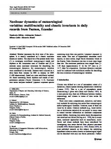
locations of the stations (Legnica, Kołobrzeg, Gdynia, Zakopane, Lesko, Warszawa) were chose so as to allow the testing of models under various climatic conditions of Poland: two of the stations are situated on the coast of the Baltic Sea, two in the mountains, and two in lowland areas in the central and the south-west part of Poland (Fig. 1, Tab. 2). The choice of the models to be tested was subjective, but conforming with the authors’ knowledge that those models should perform the best in the climatic conditions of Poland.
2 Material and methods In the study we verified selected models for the estimation of total radiation (Tab. 1) which were tested on data from 6 locations in the territory of Poland. The
*
Fig. 1. Location of measurement stations in the territory of Poland.
Corresponding author:
[email protected]
© The Authors, published by EDP Sciences. This is an open access article distributed under the terms of the Creative Commons Attribution License 4.0 (http://creativecommons.org/licenses/by/4.0/).
ITM Web of Conferences 23, 00032 (2018) XLVIII Seminar of Applied Mathematics
https://doi.org/10.1051/itmconf/20182300032
Table 1. Summary of the studied formulae.
Name
Formulae
1
Hargreaves [12]
2
Hunt et al. [11]
3
Hunt et al. [11]
4
Wu et al. [13]
5
Kuchar et al.
6
Combined [11,13,16,17]
7
Combined [16,17]
where: a, b, c, d, e, f, g – constants, – diurnal radiation totals , – extraterrestrial solar radiation – diurnal maximum temperature [°C], – diurnal minimum temperature [°C], – diurnal minimum temperature of the next day [°C], P – diurnal precipitation totals [mm], R – binary variable: “did a precipitation phenomenon occur”,
Alt [m]
Lat
Long
[°N]
[°E]
.
independently for each observation, 7 values estimating total radiation were obtained for each of the 7 formulae. Next, errors of approximation were estimated using the Coefficient of Determination (R²) and the Root Mean Squared Error (RMSE) [15].
Table 2. Sites of meteorological stations.
Station
,
Gdynia
2
54
31
8
18
33
33
Kołobrzeg
3
54
10
58
15
34
50
3 Results and Discussion
Legnica
122
51
11
33
16
12
28
Warszawa
106
52
10
10
20
58
5
Lesko
420
49
27
59
22
27
30
Zakopane
855
49
17
38
19
57
37
Comparison of the mean values of diurnal total radiation for the estimates and the observations, in division for the stations and months, is presented in Table 3. The results confirm definitively that, with the exception of estimation using model 1, the mean values of radiation estimated with the use of the presented models are equal to the monthly mean of the measured radiation (with accuracy to one decimal place, with only a few exceptions). The differences in the mean value for model 1 result from the absence of a free term in the first model. On the basis of the estimated values of radiation coefficients R² and RMSE were calculated for all stations and models, in division for the calendar months of the vegetation period (Tab. 4, Tab. 5). Dispersion graphs for the observations and the estimations with the presented models are given in Fig. 2 – 7. The estimation of diurnal total radiation attained the best results at the stations situated in the mountains, i.e. in Lesko and in Zakopane. The highest values of coefficient R² for those stations amount to as much as 0.75, with RMSE in the range of 3.9 – 4.0 for June in Lesko, and 0.75 with RMSE 2.7 for September at the station in Zakopane. Those values were obtained in estimations using models 6 and 7. At those stations, beginning with model 3, all coefficients R² are higher than 0.60, and in many cases their value exceeds 0.70. Moving on to stations situated in the lowland areas of Poland, one can note that the highest values of coefficient R², at the level of 0.75–0.76 with RMSE of 2.4 , were attained for September through
The meteorological data acquired from the Institute of Meteorology and Water Management – National Research Institute cover the 10–year period from 2001 to 2010. In the study we focused on the vegetation period, i.e. the months from April till September. The data included days with no radiation measurements, but those were less than 1% of all observations. The data for the vegetation period were divided into months and stations, i.e. every data set included data from the same station and the same calendar month. For the estimation of diurnal total radiation in the vegetation period 7 different models were chosen (Tab. 1) [11–13], the advantage of which is their simple structure, using standard meteorological data, and their availability. The models include the following variables in their description: extraterrestrial solar radiation (calculated from the formula as a function of geographic latitude, day in the year, declination of the sun, and solar constant), diurnal maximum and minimum temperature – , [°C]. The more complex models additionally take into account the information on precipitations – P [mm]. In the calculations we applied a model verification method of the Cross Validation type, in the version Leave-One-Out. The calculations were made in program R with the use of function lm [14]. In effect,
2
ITM Web of Conferences 23, 00032 (2018) XLVIII Seminar of Applied Mathematics
https://doi.org/10.1051/itmconf/20182300032
Table 3. Mean diurnal total radiation, measured and approximated .
prediction by means of models 6 and 7. Comparing the preceding models with consecutive ones one can note a considerable improvement in the quality of prediction from model number 1 above. From model number 3 the values of coefficient R² as well as of the error of estimation RMSE are at a stabilised level. Analysing the presented results one can note that the most difficult is the prediction of values of diurnal total radiation for the coastal stations (especially for Gdynia). The highest values of coefficient R², of 0.67 at RMSE 2.6 , were noted in Kołobrzeg for September (model 7). In Gdynia, the highest value of coefficient R², 0.58 at RMSE 4.5 , was obtained for May, also using 7. The results for models 4 – 7 are at a similar level. It may be of interest that, with the exception of September, at the coastal stations, in terms of the values of coefficient R² the estimation of diurnal total radiation is better when using model 1 than model 2 (at the remaining stations model 2 produces, in every month, much better results than model 1: even twice as high coefficient R² at a similar or slightly smaller error of estimation RMSE.) It should be noted, however, that in the first model (as opposed to the second) the mean value of diurnal total radiation differs from the observed value (Tab. 3).
Station/ Month
Formulae Obs.*
1
2
3
4
5
6
7
Gdynia
4 Conclusion The most important conclusions that can be drawn from the presented study are the following: The best predictions were obtained using models 6 and 7. These are a combination of the remaining models and an additionally constructed variable used in other non-linear models, analysed in the other studies [16,17]. It was noted that models 3–7 produced better results than models 1 and 2. This probably results from the fact that those models included information on precipitations. Due to the high variation of the results with regard to the station and to the model used, no best months for the prediction of radiation have been indicated. As far as the locations are concerned, the best results were obtained at the mountain stations, and the worst at the costal ones, which is a stimulus for further development of the formulae and for searching for additional variables. Due to the high interest in improving the quality of the models, and extensive literature has been created [18–33].
APR MAY JUN JUL AUG SEP Kołobrzeg
14.0 18.9 20.4 19.4 15.8 11.3
13.7 18.7 20.1 19.1 15.6 11.3
14.0 18.9 20.4 19.4 15.8 11.3
14.0 18.9 20.4 19.4 15.8 11.3
14.0 18.9 20.4 19.4 15.8 11.3
14.0 18.9 20.4 19.4 15.8 11.3
14.0 18.9 20.4 19.4 15.8 11.3
14.0 18.9 20.4 19.4 15.8 11.3
APR MAY JUN JUL AUG SEP Legnica
14.9 18.9 20.9 19.6 15.4 11.0
14.7 18.6 20.5 19.5 15.3 11.2
14.9 18.9 20.9 19.6 15.4 11.0
14.9 18.9 20.9 19.6 15.4 11.0
14.8 18.9 20.9 19.6 15.4 11.0
14.9 18.9 20.9 19.6 15.5 11.0
14.8 18.9 20.9 19.6 15.4 11.0
14.8 18.9 20.9 19.6 15.4 11.0
APR MAY JUN JUL AUG SEP Warszawa
16.0 19.1 20.9 19.8 16.8 11.9
16.2 19.3 21.1 20.1 16.9 12.2
16.0 19.1 20.9 19.8 16.8 11.9
16.0 19.1 20.9 19.8 16.8 11.9
16.0 19.1 20.9 19.8 16.8 11.9
16.0 19.1 20.9 19.8 16.8 11.9
16.0 19.1 20.9 19.8 16.8 11.9
16.0 19.1 20.9 19.8 16.8 11.9
14.6 18.5 20.0 19.5 16.0 11.3
14.9 18.8 20.3 19.7 16.1 11.6
14.6 18.5 20.0 19.5 16.0 11.3
14.6 18.5 20.0 19.5 16.0 11.3
14.6 18.5 20.0 19.5 16.0 11.3
14.6 18.5 20.0 19.5 16.0 11.3
14.6 18.5 20.0 19.5 16.0 11.3
14.6 18.5 20.0 19.5 16.0 11.3
14.2 17.7 19.2 18.9 16.8 11.1
14.6 18.1 19.7 19.3 17.0 11.5
14.2 17.7 19.2 18.9 16.8 11.1
14.2 17.7 19.2 18.9 16.8 11.1
14.2 17.7 19.2 18.9 16.8 11.1
14.2 17.7 19.2 18.9 16.8 11.1
14.2 17.7 19.2 18.9 16.8 11.1
14.2 17.7 19.2 18.9 16.8 11.1
14.1 15.6 16.4 16.7 14.5 10.1
14.5 16.0 16.9 17.2 14.8 10.5
14.1 15.6 16.4 16.7 14.5 10.1
14.1 15.6 16.4 16.7 14.5 10.1
14.1 15.6 16.4 16.7 14.5 10.1
14.1 15.6 16.4 16.7 14.5 10.0
14.1 15.6 16.4 16.7 14.5 10.1
14.1 15.6 16.4 16.7 14.5 10.1
APR MAY JUN JUL AUG SEP Lesko APR MAY JUN JUL AUG SEP Zakopane APR MAY JUN JUL AUG SEP
* – Observed
3
ITM Web of Conferences 23, 00032 (2018) XLVIII Seminar of Applied Mathematics
https://doi.org/10.1051/itmconf/20182300032
Table 4. Measures of fit (R²) in the period of vegetation. Month/ Station
Table 5. Errors of estimation RMSE
Formulae 1
2
3
4
5
6
Month/ Station
7
2
6
7
Gdynia
Gdynia APR
1
Formulae 3 4 5
.
.31
.11
.32
.36
.38
.41
.42
APR
6.0
5.8
5.1
4.8
4.7
4.5
4.5
6.5
6.4
5.6
4.9
4.9
4.6
4.5
MAY
.28
.13
.33
.50
.48
.56
.58
MAY
JUN
.27
.09
.29
.45
.45
.49
.50
JUN
7.0
6.8
6.0
5.3
5.3
5.1
5.1
JUL
.24
.08
.34
.50
.48
.54
.56
JUL
7.0
6.8
5.8
4.9
5.0
4.7
4.6
AUG
.30
.12
.29
.38
.39
.43
.45
AUG
5.2
5.1
4.6
4.3
4.2
4.1
4.0
.48
SEP
3.8
3.8
3.4
3.2
3.2
3.1
3.1
SEP
.32
.28
.40
.45
.45
.48
Kołobrzeg
Kołobrzeg APR
.42
.27
.48
.55
.57
.57
.57
APR
5.3
5.2
4.4
4.0
4.0
3.8
3.8
MAY
.42
.17
.37
.41
.43
.46
.46
MAY
6.5
6.3
5.5
5.2
5.1
5.0
5.0
JUN
.37
.08
.30
.45
.45
.49
.47
JUN
6.9
6.5
5.7
5.1
5.1
4.9
5.0
JUL
.34
.26
.50
.61
.63
.66
.65
JUL
5.9
5.8
4.8
4.2
4.1
3.9
4.0
5.0
5.0
4.2
4.0
3.9
3.7
3.7
3.4
3.3
2.9
2.8
2.7
2.6
2.6
AUG
.31
.22
.45
.47
.50
.55
.55
AUG
SEP
.36
.50
.63
.63
.64
.66
.67
SEP Legnica
Legnica APR
.41
.60
.67
.68
.72
.73
.73
APR
3.8
3.7
3.4
3.3
3.2
3.0
3.1
MAY
.33
.55
.64
.66
.67
.70
.71
MAY
4.8
4.6
4.2
4.0
3.9
3.7
3.7
JUN
.33
.45
.56
.61
.62
.66
.66
JUN
5.1
5.0
4.5
4.2
4.2
4.0
4.0
JUL
.24
.51
.58
.61
.61
.62
.62
JUL
5.0
4.7
4.4
4.2
4.1
4.1
4.1
AUG
.39
.59
.65
.67
.69
.70
.71
AUG
3.8
3.7
3.4
3.3
3.2
3.1
3.1
SEP
.45
.71
.74
.75
.76
.76
.76
SEP
2.9
2.8
2.6
2.5
2.5
2.4
2.4
Warszawa
Warszawa APR
.29
.58
.66
.67
.70
.68
.68
APR
4.2
4.0
3.6
3.4
3.4
3.4
3.4
MAY
.25
.47
.56
.60
.62
.62
.62
MAY
5.1
5.0
4.5
4.4
4.2
4.3
4.2
JUN
.24
.49
.56
.59
.60
.60
.60
JUN
4.9
4.7
4.3
4.2
4.1
4.1
4.1
JUL
.27
.54
.62
.62
.63
.63
.63
JUL
4.3
4.1
3.7
3.8
3.7
3.7
3.7
AUG
.27
.44
.53
.59
.59
.60
.60
AUG
4.1
4.0
3.7
3.4
3.4
3.4
3.4
SEP
.36
.66
.71
.73
.74
.75
.75
SEP
2.9
2.7
2.5
2.5
2.4
2.4
2.4
Lesko
Lesko APR
.27
.57
.65
.68
.70
.70
.70
APR
4.8
4.5
4.0
3.7
3.7
3.6
3.6
MAY
.27
.57
.64
.65
.66
.68
.68
MAY
5.1
4.8
4.4
4.2
4.1
4.1
4.0
JUN
.23
.61
.70
.71
.73
.75
.75
JUN
5.5
4.9
4.3
4.2
4.1
4.0
3.9
5.1
4.5
4.1
3.9
3.8
3.8
3.8
JUL
.25
.63
.70
.72
.73
.74
.74
JUL
AUG
.27
.58
.65
.67
.68
.70
.70
AUG
4.3
4.0
3.7
3.6
3.5
3.4
3.4
SEP
.34
.69
.74
.70
.71
.73
.73
SEP
3.3
3.0
2.8
2.9
2.8
2.7
2.7
Zakopane
Zakopane APR
.25
.55
.65
.64
.67
.68
.68
APR
4.7
4.4
3.9
3.9
3.7
3.7
3.7
MAY
.23
.52
.61
.69
.70
.71
.71
MAY
5.2
4.9
4.4
4.0
4.0
3.9
3.9
JUN
.21
.55
.64
.65
.67
.67
.67
JUN
5.7
5.2
4.6
4.5
4.4
4.4
4.4
JUL
.22
.61
.67
.68
.70
.70
.70
JUL
5.5
4.8
4.5
4.4
4.3
4.3
4.3
AUG
.27
.58
.66
.68
.70
.71
.71
AUG
4.1
3.8
3.4
3.3
3.2
3.2
3.2
SEP
.29
.63
.69
.73
.73
.75
.75
SEP
3.6
3.3
3.0
2.8
2.8
2.7
2.7
4
ITM Web of Conferences 23, 00032 (2018) XLVIII Seminar of Applied Mathematics
https://doi.org/10.1051/itmconf/20182300032
Fig. 2. Comparison of measured and predicted values of radiation for models 2–7 and months of AprilSeptember at station Gdynia.
Fig. 5. Comparison of measured and predicted values of radiation for models 2–7 and months of AprilSeptember at station Warszawa.
Fig. 3. Comparison of measured and predicted values of radiation for models 2–7 and months of AprilSeptember at station Kołobrzeg.
Fig. 6. Comparison of measured and predicted values of radiation for models 2–7 and months of AprilSeptember at station Lesko.
Fig. 4. Comparison of measured and predicted values of radiation for models 2–7 and months of AprilSeptember at station Legnica.
Fig. 7. Comparison of measured and predicted values of radiation for models 2–7 and months of AprilSeptember at station Zakopane.
5
ITM Web of Conferences 23, 00032 (2018) XLVIII Seminar of Applied Mathematics
https://doi.org/10.1051/itmconf/20182300032
24. X. Liu, X. Mei, Y. Li, Q. Wanga, J.R. Jensen, Y. Zhang, J.R. Porter, Agric. For. Meteorol. 149, 1433–1446 (2009) 25. M.G. Abraha, M.J. Savage, Agric. For. Meteorol. 148, 401–416 (2008) 26. J. Almorox, Turk. J. Phys. 35, 53–64 (2011) 27. F. Antonanzas-Torresa, A. Sanz-Garcia, F. J. Martínez-de-Pisón-Ascacíbar, O. PerpiñánLamigueiro, Renew. Energy 60, 604–614 (2013) 28. F. Besharat, A.A. Dehghan, A.R. Faghih, Renew. Sust. Energ. Rev. 21, 798–821 (2013) 29. Mao-Fen Li, Hong-Bin Liu, Peng-Tao Guo, Wei Wu, Energy Convers. Manag. 51, 2575–2579 (2010) 30. S. Rehman, M. Mohandes, Energy Policy 36(2), 571–576 (2008) 31. D.L. Liu, B.J. Scott, Agric. For. Meteorol. 106, 41– 59 (2001) 32. M. Trnka, Z. Žalud, J. Eitzinger, M. Dubrovský, Agric. For. Meteorol. 131, 54–76 (2005) 33. C.M. Dos Santos, J.L. De Souza, R.A. Ferreira Junior, C. Tiba, R.O. de Melo, G.B. Lyra, I. Teodoro, G.B. Lyra, M.A.M. Lemes, Energy 71, 388–398 (2014)
References 1. 2. 3. 4.
5. 6. 7. 8. 9. 10. 11. 12.
13. 14. 15.
16. 17.
18. 19.
20.
21. 22. 23.
S. Bac, S. Iwański, L. Kuchar, Acta Agrophys. 12(2), 305–314 (2008) J. Lu, G. Sun, S. G. McNulty, D. M. Amatya, J. Am. Water Resour. As. 41(3), 621–633 ( 2005) R. Fischer, J. Agric. Science 105(2), 447–461 (1985) N. Deng, X. Ling, Y. Sun, C. Zhang, S. Fahad, S. Peng, K. Cui, L. Nie, J. Huang, Eur. J. Agron. 64, 37–46 (2015) P. Garofalo, M. Rinaldi, Europ. J. Agronomy 64, 88–97 (2015) A. Granier, N. Bre´da, P. Biron, S. Villette, Ecol. Modell. 116, 269–283 (1999) P. Döll, F. Kaspar, B. Lehner, J. Hydrol. 270, 105– 134 (2003) M. Šúri, J. Hofierka, Trans. GIS 8(2), 175–190 (2004) M. Šúri, T. A. Huld, E. D. Dunlop, H. A. Ossenbrink, Sol. Energy 81(10), 1295–1305 (2007) F. Evrendilek, C. Ertekin, Clim. Dyn. 31, 131–149 (2008) L.A. Hunt, L. Kuchar, C.J. Swanton, Agric. For. Meteorol. 91, 293–300 (1998) G. H. Hargreaves, Responding to tropical climates, The 1980–81 Food and Climate Review, The Food and Climate Forum (Aspen Institute for Humanistic Studies, Boulder, Colo), 29–32 (1981) G. Wu, Y. Liu, T. Wang, Energy Convers. Manag. 48, 2447–2452 (2007) G. Daròczi, Mastering Data Analysis with R (Birmingham, Packt Publishing, 2015) R.E. Walpole, R.H. Myers, Probability and Statistics For Engineers and Scientists (New York, McMillan, 1972) K.L. Bristow, G.S. Campbell, Agric. For. Meteorol. 31, 159–166 (1984) M. Donatelli, G.S. Campbell, Proc. ESA Congr., 5th, Nitra, Slovak Republic (28 June–2 July 1998, The Slovak Agric. Univ., Nitra, Slovak Republic), 133–134 (1998) L. Kuchar, S. Iwański, L. Jelonek, W. Szalińska, Geografie 119, 1 (2014) L. Kuchar, S. Iwański, L. Jelonek, E3S Web of Conf. 17, 00046 (2017) doi: 10.1051/e3sconf/20171700046 L. Kuchar, S. Iwański, L. Jelonek, W. Szalińska, Meteorol. Hydrol. Water Manage. 2, 49 (2014) S.E. Hollinger, L. Kuchar, Math. Comp. Symul. 42, 2–3, 293 (1996) L. Kuchar, Int. Agrophys. 8(3), 525 (1994) A. Dumas, A. Andrisani, M. Bonnici, G. Graditi, G. Leanza, M. Madonia, M. Trancossi, Sol. Energy 116, 117–124 (2015)
6