Biogeosciences, 9, 2537–2564, 2012 www.biogeosciences.net/9/2537/2012/ doi:10.5194/bg-9-2537-2012 © Author(s) 2012. CC Attribution 3.0 License.
Biogeosciences
How errors on meteorological variables impact simulated ecosystem fluxes: a case study for six French sites Y. Zhao1 , P. Ciais1 , P. Peylin2 , N. Viovy1 , B. Longdoz3 , J. M. Bonnefond4 , S. Rambal5 , K. Klumpp6 , A. Olioso7,8 , P. Cellier9 , F. Maignan1 , T. Eglin1 , and J. C. Calvet10 1 Laboratoire
des Sciences du Climat et de l’Environnement, UMR8212, CEA-CNRS-UVSQ, 91191 Gif-sur-Yvette, France de Biog´eochimie Isotopique, LBI, Bˆatiment EGER, 78026 Thiverval-Grignon, France 3 INRA, Centre INRA de Nancy, UMR1137, Ecologie et Ecophysiologie Foresti` eres, 54280 Champenoux, France 4 INRA, UMR1263, EPHYSE, 33140, Villenave d’Ormon, France 5 Dream CEFE-CNRS, 1919 route de Mende, 34293 Montpellier, France 6 INRA, Grassland Ecosystem Research, 234 Avenue du Br´ ezet, Clermont-Ferrand, 63039, France 7 INRA, UMR1114, EMMAH, Domaine Saint-Paul, 84914 Avignon Cedex 9, France 8 UAPV, UMR1114, EMMAH, 33, Rue Lois pasteur, 84000, Avignon, France 9 INRA, UMR1091, Environnement et Grandes Cultures, 78850 Thiverval-Grignon, France 10 CNRM/GAME, M´ et´eo-France, CNRS, 42 avenue Coriolis, 31057 Toulouse Cedex 1, France
2 Laboratoire
Correspondence to: Y. Zhao (
[email protected]) Received: 29 November 2010 – Published in Biogeosciences Discuss.: 9 March 2011 Revised: 29 April 2012 – Accepted: 7 May 2012 – Published: 11 July 2012
Abstract. We analyze how biases of meteorological drivers impact the calculation of ecosystem CO2 , water and energy fluxes by models. To do so, we drive the same ecosystem model by meteorology from gridded products and by meteorology from local observation at eddy-covariance flux sites. The study is focused on six flux tower sites in France spanning across a climate gradient of 7–14 ◦ C annual mean surface air temperature and 600–1040 mm mean annual rainfall, with forest, grassland and cropland ecosystems. We evaluate the results of the ORCHIDEE process-based model driven by meteorology from four different analysis data sets against the same model driven by site-observed meteorology. The evaluation is decomposed into characteristic time scales. The main result is that there are significant differences in meteorology between analysis data sets and local observation. The phase of seasonal cycle of air temperature, humidity and shortwave downward radiation is reproduced correctly by all meteorological models (average R 2 = 0.90). At sites located in altitude, the misfit of meteorological drivers from analysis data sets and tower meteorology is the largest. We show that dayto-day variations in weather are not completely well reproduced by meteorological models, with R 2 between analysis data sets and measured local meteorology going from 0.35
to 0.70. The bias of meteorological driver impacts the flux simulation by ORCHIDEE, and thus would have an effect on regional and global budgets. The forcing error, defined by the simulated flux difference resulting from prescribing modeled instead of observed local meteorology drivers to ORCHIDEE, is quantified for the six studied sites at different time scales. The magnitude of this forcing error is compared to that of the model error defined as the modeled-minusobserved flux, thus containing uncertain parameterizations, parameter values, and initialization. The forcing error is on average smaller than but still comparable to model error, with the ratio of forcing error to model error being the largest on daily time scale (86 %) and annual time scales (80 %). The forcing error incurred from using a gridded meteorological data set to drive vegetation models is therefore an important component of the uncertainty budget of regional CO2 , water and energy fluxes simulations, and should be taken into consideration in up-scaling studies.
Published by Copernicus Publications on behalf of the European Geosciences Union.
2538 1
Introduction
The terrestrial biosphere is a key component of the global carbon cycle that receives large attention in terms of climate change mitigation because of its current carbon sink (Prentice et al., 2001; Schimel et al., 2001) and because of potential positive feedbacks with future climate change (Friedlingstein et al., 2006). Process oriented Terrestrial Biosphere Models (TBMs) are useful tools to quantify and understand carbon flux and pool variability at a range of spatial scales, and to predict the response of ecosystems in response to climate and environmental changes. Global or regional meteorological fields on a grid, generated by numerical weather prediction models such as the European Center for Medium-Range Weather Forecasts (ECMWF) or the National Center for Environmental Precipitation (NCEP), or by optimal data interpolation schemes (Mitchell et al., 2009), are commonly used to drive TBMs for regional and global applications. Weather is the main driver of variations in CO2 , H2 O and heat fluxes on short time scales going from days to months (Mahecha et al., 2007). Climate plays a key role in interaction with biotic drivers by controlling fluxes on a seasonal to interannual time scale (Knorr et al., 2005; Peylin et al., 2005; Ciais et al., 2005; Richardson et al., 2007). One of the first studies acknowledging that bias in meteorological drivers affected the estimation of photosynthesis (GPP) by models at regional scale is the one of Jung et al. (2007). They found GPP differences over Europe of 34 % on a seasonal time scale and of 40–60 % on an interannual timescale, given different drivers. However, how bias in meteorology translates into uncertainty on Net Ecosystem Exchange (NEE), Latent Heat (LH) and Sensible Heat (SH) fluxes has rarely been investigated in a systematic approach (Riccuito et al., 2009; Sczcypta et al., 2011). To tackle this problem, we use continuous measurements of CO2 , H2 O and heat fluxes made by an eddy-covariance technique at six flux tower sites in France. The six sites cover three forests, two croplands and one grassland site, growing under contrasted climate conditions. The choice of France as a case study to analyze the effects of meteorological driver biases can be justified because a high-resolution meteorological forcing, SAFRAN (Durand et al., 1993, 1999), is available over the country from the French meteorological service M´et´eo-France on a 8 km by 8 km grid. The SAFRAN regional high resolution forcing can be compared with other products from coarser resolution global weather analyses commonly prescribed as input to TBMs. The TBM used in this study is ORCHIDEE, a processoriented model that simulates ecosystem processes and resulting carbon, water and energy fluxes at the time step of a half-hour. This allows explicit calculation of the diurnal variation of ecosystem fluxes and consistency with the 30 min acquisition time step of flux data (Baldocchi et al., 2001; Reichstein et al., 2005). At each eddy-covariance site, meteorological parameters are measured together with CO2 , H2 O, Biogeosciences, 9, 2537–2564, 2012
Y. Zhao et al.: A case study for six French sites and heat fluxes. Site observed meteorology will serve as a basis against which meteorological analysis data sets can be compared. For applications limited to sites, local meteorology is the best possible driver for TBMs, although it contains uncertainty (Sect. 2.3) and scale mismatch with the footprint of eddy-covariance measurements (Baldocchi et al., 2001). For modeling regional carbon budgets, meteorological forcing is needed on a grid; hence, modelers cannot avoid using imperfect model data sets. Although there is a scale issue between local observations and gridded data from meteorological models, the comparison at site scale is crucial to assess model performance at regional scale. The goal of this study is to investigate how the errors on meteorological variables impact simulated ecosystem fluxes. In specific, we address the following questions: 1. How different is meteorology at flux tower locations between local observation and gridded data-products: change to data sets? 2. Is the error of modeled meteorology random or systemic? 3. What is the uncertainty of simulated ecosystem CO2 , water vapour and heat fluxes (here using the ORCHIDEE model) induced by errors in meteorological drivers relative to model errors? 4. What is the sensitivity of ecosystem fluxes simulated by ORCHIDEE to each specific meteorological driver? These questions are investigated for Net Ecosystem Exchange (NEE), photosynthesis (GPP), Total Ecosystem Respiration (TER), latent (LH) and sensible heat fluxes (SH). The time scales investigated go from hour to year, yet focus on the growing season period. 2
Material and methods
2.1
Eddy-covariance data from six flux towers
The six sites (Table 1) cover a deciduous broad-leaved beech forest (Hesse), a temperate needle-leaved maritime pine forest (Le Bray), a Mediterranean green oak forest (Pu´echabon), an extensively managed grassland (Laqueuille), and two intensive cropland sites, one in the Paris region (Grignon) and one in the south of France (Avignon). The sites’ climate space distribution over France is shown in Fig. 1. The entire data set represents a total of 42 site x years (Table 1). – Hesse (HES) is a 40-yr old beech forest in the northeast of France. The growing season spans from 1 May to mid-October. The forest is thinned each 4–5 yr, and approximately 20 % of the basal area is removed each time. The measured stand was thinned in the winters of 1995/1996, 1999/2000 and 2004/2005.
www.biogeosciences.net/9/2537/2012/
Y. Zhao et al.: A case study for six French sites
2539
Table 1. Summary of eddy flux observation sites used in this study. Site name
Hesse (HES)
Le Bray (LBR)
Pu´echabon (PUE)
Laqueuille (LQE)
Avignon (AVI)
Grignon (GRI)
Vegetation Class
90 % DBF, 10 % grass
80 % ENF, 20 % grass
90 % EBF, 10 % soil
C3 grass
crop
crop
Dominant Species (Age)
Beech (40 yr)
maritime pine (40 yr)
Mediterranean green oak (70 yr)
Extensively grazed grassland
Rotation, wheat-peassorghum
Rotation maizewheatbarley
Mean annual Biomass (gC m2 )
7000
7850
16 600
300
400
225
Location
7.06◦ E, 48.67◦ N
−0.77◦ E, 44.72◦ N
3.6◦ E, 43.74◦ N
2.75◦ E, 45.64◦ N
4.88◦ E, 43.92◦ N
1.95◦ E, 48.84◦ N
Elevation (m)
300
61
270
1040
32
125
Mean annual temperature(◦ C)
14,2
13,2
13,2
7,4
14,2
11,1
Annual precipitation (mm)
975
972
900
1081
480
600
Observation Period
1997–2007
1996–2007
2000–2007
2004–2007
2004–2007
2005–2007
Annual NEE (gC m2 )
335
365
235
245
155
235
References
Longdoz et al. (2008)
Delzon and Loustau (2005) Jarosz et al. (2008)
Rambal et al. (2003)
Soussana et al. (2004)
Olioso et al. (2005)
Cellier et al. (2002)
– Le Bray (LBR) is an even-aged maritime pine forest seeded in 1970, part of the Les Landes forest near the Atlantic ocean. The growing season is almost all year round. The site is managed according to a standard local management strategy and was thinned in 1991, 1996 and 2004. – Pu´echabon (PUE) is a 70-yr old Holm oak forest, typical of Mediterranean southeastern France. It has a Mediterranean climate type. Rainfall mainly occurs during fall and winter with about 80 % between September and April; the summer is very dry. The growing season goes mostly from March to mid-August. – Laqueuille (LQE) is an extensively managed grassland located in Massif Central (central France). The growing season goes from the end of April until October. During that period the grassland is lightly grazed continuously and no fertilizer is applied. – Avignon (AVI) is a long established agricultural site located in southeastern France. Durum wheat, peas and durum wheat are the rotation crops grown during 2003/2004, 2004/2005 and 2005/2006, respectively. All www.biogeosciences.net/9/2537/2012/
are winter crops and their harvest date is at the end of June. In 2007 sorghum, a C4 summer crop, was grown and harvested in the middle of October. Irrigation is applied in particular to sorghum and peas. In the following, we focus the comparison of AVI fluxes with ORCHIDEE simulations (winter C3 crop type) for the periods of winter crop cultivation. – Grignon (GRI) is an intensive cropland site situated in the Paris area. The rotation was maize-wheat-barley in 2005, 2006 and 2007, with mustard as an intercrop between barley and maize. Maize is seeded by early May and harvested at the end of September. Wheat and barley are seeded in the middle of October and harvested around early-to-mid July. The site is managed with superficial tillage and a slurry application every three years at mustard sowing. The growing season (GS) and peak growing season (PGS) are site- and definition- dependent. We define GS as the period going from 1 May to 30 September for all sites, except for PUE where it is from 1 March to 31 August. The PGS, the two-month period after GPP reaches its peak, spans from Biogeosciences, 9, 2537–2564, 2012
2540
Y. Zhao et al.: A case study for six French sites
98
(http://gaia.agraria.unitus.it) for CO2 fluxes, SH, LH and all meteological parameters except longwave radiation, which was complementarily provided by each site manager. Level4 data sets are used for the study, in which flux separation techniques for splitting the observed net carbon fluxes into assimilation and respiration have been employed (Reichstein et al., 2005). 2.2 2.2.1
99 100 101 102 103 104 105 106
Fig. 1. The ecosystem types (DBF = deciduous broad-leaved forEBF = evergreen broad-leaved forest, ENF = evergreen needleleaved forest, CRO = cropland, GRA = grassland) of six selected flux sites over France in the climatic space: mean temperature versus annual precipitation, which are calculated as the mean of SAFRAN results over 1994 to 2007. The observed mean temperature and annual precipitation at each site is indicated. The six sites are: Hesse (HES), Pu´echabon (PUE), La Bray (LBR), Laqueuile (LQE), Avignon (AVI) and Grignon (GRI).
Figure 1est,
107 108 109
1 July to 31 August for HES, LBR and LQE, and 1 May to 30 June for PUE, AVI and GRI. All sites are equipped to measure NEE, SH and LH by the covariance technique at every 30 min time step (Baldocchi et al., 2001). Meteorological data were continuously measured and averaged every half-hour. Because flux measurements are affected by (1) both random and systematic (bias) errors, which arise from limitations of the measurement technique, (2) the stochastic nature of turbulence, and (3) site-specific differences in data processing protocols (Moncrieff et al., 1996; Papale et al., 2006; Richardson et al., 2006, 2008), quality checks of the data were done according to CarboEurope-IP guidelines (Aubinet et al., 2000). Gap-filling was performed according to the marginal distribution sampling (MDS) method (Reichstein et al., 2005), for which uncertainties were quantified in gap-filling by Moffat et al. (2007). The MDS technique showed a consistently good gap-filling performance and low annual sum bias. According to the study of Moffat et al. (2007), the gap-filling techniques are already at or very close to the noise limit of the measurements and the effects of gapfilling on the annual sums of NEE are modest (∼50 gC m−2 yr−1 ). The flux tower data were downloaded from the Carboeurope-IP database Biogeosciences, 9, 2537–2564, 2012
ORCHIDEE model Model description
The ORCHIDEE terrestrial biosphere model describes the carbon, energy and water fluxes, (Krinner et al., 2005) and ecosystem carbon and water dynamics. It contains three submodules: a land surface energy and water balance model, SECHIBA (de Rosnay and Polcher, 1998; Ducoudr´e et al., 1993); a land carbon cycle model, STOMATE; and a model of long-term vegetation dynamics that includes competition and disturbances, adapted from Sitch et al. (2003). In this study, prescribed vegetation is used at each site (5 plant functional types (PFT) – see Table 1 – being relevant in this study). The half-hourly energy and water balance of vegetated and non-vegetated surfaces, as well as canopy-level photosynthesis, is modeled by using coupled leaf-level photosynthesis and stomatal conductance equations (Ball et al., 1987; Farquhar et al., 1980). Stomatal conductance is reduced by the soil water stress (McMurtrie et al., 1990) function of soil moisture and root profiles. Two soil water reservoirs are considered, a surface reservoir which refills in response to rain events and which is brought to zero during dry periods, and a deeper bucket reservoir of 2 m depth updated from evaporation, root uptake, percolation and runoff on a daily time scale. Autotrophic respiration is modeled at a half-hourly time 5 step, and plant growth, mortality, soil carbon decomposition and phenology at a daily time step. Leaf onset is calculated as a function of growing degree-days and chilling days requirements, or as a function of soil moisture changes specific to each PFT (Botta et al., 2000). Assimilated carbon can be allocated to stems, leaves, fruits, carbohydrate reserves, fine and coarse roots. Allocation is controlled by phenology, and by light availability, temperature and soil water (Friedlingstein et al., 1999). Autotrophic respiration is the sum of temperature-dependent maintenance respiration processes and GPP-dependent growth respiration processes. Litter and soil organic matter decomposition are calculated on a daily time step using first-order kinetics for decay of 5 C pools based upon the CENTURY model equations (Parton et al., 1988). 2.2.2
Model set-up for site simulations
ORCHIDEE is run at each site, driven by meteorological data (see Sect. 2.3.1 for the required meteorological variables). www.biogeosciences.net/9/2537/2012/
Y. Zhao et al.: A case study for six French sites The fractional coverage of PFT at each site is prescribed according to site species data (Table 1). Each simulation includes an equilibrium spin-up run followed by a transient run. In the spin-up run, observed meteorology for the period of observation is used cyclically to drive the model for 1500 yr until equilibration of carbon (and water) pools is attained, with / < Bmodel >
(3)
RHmodel opt = RHmodel . < TERobs − RAM model opt − RAGmodel > / < RHmodel >
(4)
TERmodel opt = RHmodel opt + RAGmodel + RAM model opt (5) We apply this optimization procedure to all sites except PUE. The observed total biomass provided by each site manager is www.biogeosciences.net/9/2537/2012/
Y. Zhao et al.: A case study for six French sites 30 25
Tair(°C)
Hourly
HES
25
20
20
15
15
Daily
Monthly
Annual 16 14 12 10 8
10
14 12 10 8 6
14 12 10 8 6
10
8
8
7
6
6
4
5
8 6 4 2 0
7
6 5 4 3 2 1
600
0
350 300 250 200 150 100
300 250 200 150 100 50
450
450
400
450
400
400
375
400
350
350
300
325
250
300
Rain(mm/d)
Qair(g/gk)
10
SW(w/m2)
25 20 15 10 5 0
LW(w/m2)
30
2543
800 400 200
350
350
300
300
30
30
25
25
20
20
LW(w/m2)
SW(w/m2)
Rain(mm/d)
Qair(g/gk)
LBR
Tair(°C) Qair(g/gk)
Aug
375 350
350
300
300
325
300
250
J MM J S N
97 00 03 06
25 20 15 10 5 0
16 14 12 10 8
5 3 1
30
25
25
20
20
15
15
10
10
14 12 10 8 6
600 400
140
200
120
0
450
400
450
400
375
400
350
350
350
350
300
300
300
325
250
300
Aug
30
J MM J S N 16 14 12 10 8
14 12 10 8 6
10
8
8
7
6
6
4
5
8 6 4 2 0
7
6 5 4 3 2 1
350 300 250 200 150 100
300 250 200 150 100 50
5 3 1
SW(w/m2)
450
450
400
400
350
350
350
350
300
300
325
300
250
300
Jul
Aug
LOCAL SAFRAN
7
6
6
4
5
8 6 4 2 0
7
6 5 4 3 2 1
350 300 250 200 150 100
300 250 200 150 100 50
5 3 1
180 160 140 120
450
400 375 350
300
300
325
300
250
Jul
30
30
25
25
20
20
15
15
10
10
14 12 10 8 6
200 0
EC−OPERA ERA−I
8
8
350
120
97 00 03 06
10
350
400
J MM J S N
14 12 10 8 6
350
600
375
97 00 03 06 16 14 12 10 8
400
140
400
300
J MM J S N
400
160
400
120
450
180
450
140
400
800
600
160
25 20 15 10 5 0
6 12 18
GRI
Aug
180
450
97 00 03 06
25 20 15 10 5 0
Jul
30
160
400
6 12 18
AVI
180
450
0
6 12 18
800
Jul
1
350
300 250 200 150 100 50
200
300 250 200 150 100 50
3
400
350 300 250 200 150 100
400
6 5 4 3 2 1
5
350
6 5 4 3 2 1
800
7
400
7
14 12 10 8 6
5
8 6 4 2 0
400
8 6 4 2 0
10
6
4
400
5
10
7
6
450
4
15
8
8
450
6
20
10
450
6
25
14 12 10 8 6
0
7
15
10
14 12 10 8 6
120
8
20
15
10
200
10
25
20
15
140
8
30
20
400
14 12 10 8 6
0
Annual 16 14 12 10 8
600
14 12 10 8 6
200
Monthly 25 20 15 10 5 0
160
10
400
Daily
25
180
15
600
30
350 300 250 200 150 100
10
800
Hourly
800
LW(w/m2)
Rain(mm/d)
1
15
6 12 18
PUE
3
Jul
Tair(°C)
6 12 18
5
LQE 30 25
Aug
300
J MM J S N
97 00 03 06
25 20 15 10 5 0
16 14 12 10 8
14 12 10 8 6
10
8
8
7
6
6
4
5
8 6 4 2 0
7
6 5 4 3 2 1
350 300 250 200 150 100
300 250 200 150 100 50
5 3 1
180 160 140 120
450
400
450
400
375
400
350
350
350
350
300
300
325
300
250
450 400
6 12 18
Jul
Aug
300
J MM J S N
97 00 03 06
REMO Calculated LW
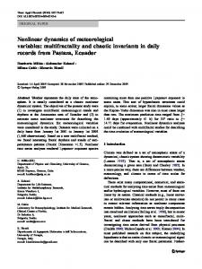
Fig. 2. Meteorological drivers in in situ and in gridded data sets at six sites. First column: hourly mean diurnal cycle over peak growing season (PGS). Second column: daily mean with a running mean of 3 days for July–August of 2003 at HES, LBR and PUE and of 2005 for LQE, AVI and GRI. Rainfall is calulated as 5-day aggregated values: third column: monthy mean seasonal cycle; fourth column: annual mean. The hourly mean diurnal cycle and monthly mean seasonal cycle correspond to 2004–2007 except for EC-OPERA (2003 to 2006). In the case of site-year without measured LWdown , calculated LWdown is plotted in dash lines. See text Sect. 2.1 for the definiton of PGS.
www.biogeosciences.net/9/2537/2012/
Biogeosciences, 9, 2537–2564, 2012
2544
Y. Zhao et al.: A case study for six French sites
7000, 7850, 300, 400 and 225 gC m−2 yr−1 at HES, LBR, LQE, AVI and GRI, respectively. The biomass disequilibrium factors are respectively 0.35, 0.55, 0.45, 0.58 and 0.27, and the soil disequilibrium factors are respectively 0.60, 0.77, 0.85, 0.67 and 0.30 at these five sites. In other words, heterotrophic respirations are overestimated by ORCHIDEE from 18 % at LQE to 220 % at GRI. This optimization procedure for TER is not applied to the Mediterranean forest site PUE because the overestimated TER at this site is caused by both discrepancies in carbon allocation between root and aboveground reservoirs and the equilibrium assumption: calculation from the above procedure would give negative RHmodel opt , which is not realistic. We thus simply optimized the simulated TER with the average observed TER. The ratio of averaged observed to simulated TER is about 0.67, indicating that TER is overestimated by ORCHIDEE by about 49 % at PUE. Thus NEE is optimized for all six sites according to NEEmodel opt = TERmodel opt − GPPmodel .
(6)
In the study, the optimized TER and resulting NEE are presented and discussed without specification.
water fluxes, because conversion of daily to hourly forcing is common practice for TBMs. The average diurnal cycles of Tair and SWdown are well simulated by all gridded products, with R 2 from 0.51 to 0.97 (p < 0.01) (Fig. 3). The daytime values of Tair between 06:00 and 19:00 UMT appear, however, to be overestimated at the forest sites, but within 2 ◦ C of local observations at the crop sites. This may reflect local evaporative cooling over forests (Zaitchik et al., 2006; Teuling et al., 2010). The pronounced diurnal cycle of Qair presented in REMO is found neither in LOCAL, nor in any other gridded data set. This spurious diurnal amplitude is most likely caused by our conversion of daily to hourly values, rather than a structural bias of the REMO physics (Campbell and Norman, 1998). The observed LWdown diurnal amplitude (≈40 Wm−2 ) at LBR, PUE, AVI and GRI is underestimated by SAFRAN, EC-OPERA and ERA-I, which give values of 22, 26 and 34 Wm−2 , respectively, while it is overestimated by Eq. (1) when applied to daily REMO output (60 Wm−2 ). At LBR, HES and GRI, the diurnal cycle of LWdown in SAFRAN is opposite to that of other models. 3.2
3
Comparing gridded meteorology forcing against flux tower data
Figure 2 shows a comparison between observed (LOCAL) and modeled meteorology from hourly to interannual time scales based on aggregated time series Xi (i = 1, 4). Due to the short length of records, some sites were excluded: GRI, where the first year of observations is 2005 and whereas ECOPERA forcing data is only available till 2006. Figure 3 shows the R 2 of LOCAL vs. gridded meteorology on different time scales (Eq. 2). Figure 4 shows the MAE; hourly and daily statistics are calculated only during the PGS, and monthly statistics during the GS. 3.1
Hourly time scale
Strictly speaking, the analyses-observation comparison on an hourly time scale is only appliable to SAFRAN set because the time resolutions in the other three gridded sets are lower than hourly (Table 2). However, ORCHIDEE includes an interpolator to convert 6-h or less into half-hours; that is, the coarse time step of SWdown is converted into half-hourly time steps as a function of solar zenithal and site location. The other meteorological variables are linearly interpolated between two measured times. Daily time series (in the case of REMO) are disaggregated into a half-hourly scale following the procedure described in Sect. 2.3.1 for gap-filling, when downscaling daily to half-hourly is required. Thus, analysesobservation comparison on an hourly scale provides an opportunity for insight on how good the conversion procedure from coarse time scale to half-hourly is, and whether the spurious behavior has any impact on the simulated carbon and Biogeosciences, 9, 2537–2564, 2012
Daily time scale
Comparison between tower data and gridded model products is focused on the summer 2003 heat-wave (July–August) period at HES, LBR and PUE, and on summer 2005 at LQE, AVI and GRI (Fig. 2). The main result is that the synopticscale variability of daily Tair , Qair and SWdown is well captured by all gridded data sets when compared to LOCAL. For daily variability of Tair during July–August 2003 or 2005, the mean R 2 of LOCAL and models is 0.87 (from 0.79 in REMO to 0.94 in SAFRAN, p < 0.01). The synoptic variability of Tair is best captured at HES, where the mean R 2 of the four models is 0.96. The July–August mean Tair at LQE is overestimated by all models, from 1.1 ◦ C in SAFRAN to 4.2 ◦ C in ERA-I. This summer bias must be compared to the annual mean Tair bias of 0.8 ◦ C in SAFRAN and 3.3 ◦ C in ERA-I, due to unresolved topography. Concerning Rainfall, SAFRAN is in good agreement with LOCAL for daily values during July–August at all sites, except for LBR. At LBR, SAFRAN produces a mean Rainfall of 101 mm against 23 mm only in LOCAL, but the rain gauge data quality was poor during 2002 to 2006 due to instrumental failure (Loustau, personal communication, 2010). The mean summer 2003 Rainfall is 71 mm in SAFRAN and 75 mm in LOCAL across the six sites, excluding LBR. REMO overestimates Rainfall by 80 mm in summer 2003, which would cause problems for simulating the response of plants to drought during the dry 2003 summer. The daily variability of Qair is characterized by overall mean R 2 values between models and LOCAL of 0.72, REMO having the lowest correlation (0.44) and SAFRAN the highest (0.86). The AVI site has the highest R 2 between observed and modeled Qair during July–August 2005 (R 2 = 0.90, p < 0.01). The LQE www.biogeosciences.net/9/2537/2012/
Y. Zhao et al.: A case study for six French sites
2545
R2: Meteor. Analysis vs. Local Obs. Daily
Monthly
Annual
0.92
0.91
0.72
0.97
0.95
0.96
0.69
0.99
0.99
0.99
0.95
0.96
0.97
LBR 0.89
0.86
0.9
0.67
0.93
0.85
0.91
0.66
0.94
0.97
0.99
0.91
0.56
0.72
PUE 0.93
0.91
0.91
0.74
0.94
0.74
0.66
0.59
0.99
0.98
0.98
0.95
0.94
0.7 −
LQE 0.81
0.81
0.8
0.51
0.97
0.94
0.92
0.68
0.98
0.98
0.96
0.88
AVI 0.96
0.95
0.93
0.8
0.99
0.95
0.83
0.66
1
0.99
0.97
0.95
GRI 0.92
0.95
0.9
0.77
0.98
0.97
0.88
0.77
0.97
0.97
0.91
0.9
HES 0.35
0.29
0.37
0.06
0.81
0.79
0.82
0.54
0.9
0.93
0.93
0.79
0.32
0.31
0.88
0.8
0.84
0.4
0.95
0.96
0.98
0.91
0.45 − 0.29 −−
0.81
LBR 0.33 PUE 0.68
0.4
0.37
0
0.95
0.86
0.86
0.41
0.98
0.97
0.98
0.79
0.36 −−
0.37 − 0.27 −− 0.29 −− 0.29 −− 0.52 −
LQE 0.43
0.23
0.2
0.08
0.63
0.56
0.45
0.34
0.66
0.67
0.66
0.61
0.02
0.96
0.91
0.82
0.5
0.97
0.98
0.97
0.75
0.93
0.92
0.72
0.46
0.96
0.98
0.95
0.87
0.45
0.37 −
0.07 −−
0.96
0.33
0.39 −
0.72
0.48
0.9
0.6 0.06 −− 0.09 −− 0.46 −− 0.5 −
AVI 0.75
0.54
0.4
GRI 0.5
0.41
0.08
0.04 −
0.02 −−
0.9 0.78
0.04
0.04
0.5
0.22
0.23
0.11
0.87
LBR 0.12
0.08
0.04
0.4
0.22
0.2
0.07
0.7
0.13 −
PUE 0.21
0.15
0
0.49
0.33
0.19
0.13
0.92
0.77
0.8
0.65
LQE 0.41
0.05
0.04
0.68
0.26
0.18
0.09
0.86
0.68
0.49
0.33
AVI 0.34
0.04
0.07
0.68
0.55
0.6
0.17
0.99
0.87
0.15
0.06
0.65
0.47
0.4
0.14
0.71
0.91 0.35 −− 0.43 −
0.51
GRI 0.13 HES 0.88
0.94
0.94
0.86
0.63
0.67
0.7
0.38
0.97
0.95
0.98
0.91
0.06 −−
0.57
LBR 0.91
0.94
0.95
0.89
0.52
0.4
0.47
0.12
0.92
0.98
0.97
0.84
0.33
0.72
PUE 0.94
0.95
0.94
0.91
0.54
0.55
0.38
0.19
0.94
0.97
0.96
0.85
0.83
0.57 0.23 −− 0.54 −
LQE 0.8
0.76
0.74
0.74
0.42
0.34
0.22
0.14
0.69
0.72
0.69
0.49
AVI 0.96
0.97
0.96
0.94
0.75
0.62
0.51
0.27
0.96
0.98
0.96
0.92
GRI 0.9
0.95
0.95
0.87
0.59
0.74
0.69
0.33
0.96
0.99
0.98
0.85 0.52 −
0.39 −
0.06 −−
HES LBR 0.03
0.61
0.7
0.28
0.4
0.74
0.76
0.17
0.79
0.98
0.96
0.69
PUE 0.03
0.33
0.35
0.32
0.5
0.47
0.43
0.18
0.63
0.7
0.71
0.59
0.63
0.65 −
0.36
0.68
0.85
0.8
0.14
0.82
0.97
0.97
0.72
0.59
0.37
0.25
0.75
0.64
0.24
0.83
0.95
0.74
0.54
ERA−I
REMO
SAFRAN
EC−OPERA
ERA−I
REMO
SAFRAN
EC−OPERA
ERA−I
REMO
0.0
0.2
0.4
0.6
0.8
REMO
0.5
0.63
ERA−I
0.56
GRI 0.02
SAFRAN
AVI 0.08
EC−OPERA
LQE
SAFRAN
LWdown
0.6
HES 0.13
EC−OPERA
SWdown
Rainfall
Qair
Tair
Hourly
HES 0.89
1.0
Fig. 3. Squared correlation (R 2 ) between meteorological gridded data and in situ data over 2004 to 2007, except for EC-OPERA which covers 2004–2006. Panels of R 2 from left to right are for hourly, daily, monthly and annual time scales, respectively. Time series used to calculate R 2 correspond to growing season (GS). See text Sect. 2.1 for the definiton of GS. The default statistical confidence level of R 2 is p < 0.01. Otherwise, the signal “–” at the upright indicates a confidence level of p < 0.05 and “– –” for p > 0.05.
site has the smallest R 2 (0.20, p < 0.01), with low Qair observed during July, and early August being captured by none of the models. The daily variability of SWdown has a mean R 2 across the six sites of 0.49, with a range going from 0.27 in REMO to 0.68 in EC-OPERA. The HES forest has the highest R 2 for SWdown (0.63) and the PUE Mediterranean forest the lowest (0.32). But the value of R 2 between LOCAL and analysis data is lower for SWdown than for Tair or Qair , and thus errors in SWdown will be a concern in driving TBM models like ORCHIDEE by gridded products (see Sect. 5.4). The LWdown daily variability is well represented by SAFRAN, EC-OPERA and ERA-I, with R 2 values going from 0.55 (p < 0.01) in SAFRAN to 0.78 (p < 0.01) in EC-OPERA across the sites at which LWdown measure-
www.biogeosciences.net/9/2537/2012/
ments were collected during summer 2003; REMO gives poor performances (R 2 = 0.25, p < 0.01). Observed LWdown (excluding gap-filling values) in summer 2003 and 2005 is about 365 W m−2 , which is about 5 % (p < 0.01) underestimated by SAFRAN, EC-OPERA and ERA-I, but 18 % overestimated by REMO (p < 0.01). 3.3
Monthly time scale
The mean seasonal cycle of Tair , Qair , SWdown and LWdown is well captured by all gridded products (Fig. 2), with mean R 2 above 0.95 (df = 10, p 0.05) for Tair , Qair , Rainfall and SWdown , respectively (Fig. 3). A conclusion can not be made for LWdown as there is only one site (LBR) with long observed records, but R 2 tends to be low (0.40–0.65). The main result is that the weather models are only able to reproduce correctly, i.e. R 2 and p < 0.01, the interannual variablity of Tair , but the variability of other drivers is poorly captured. In particular, the interannual variability of SWdown is not well reproduced. The interannual variability of Rainfall is faithfully reproduced at HES (R 2 = 0.96, p < 0.01) and PUE (R 2 = 0.90, p < 0.01) by SAFRAN. This gives higher confidence in SAFRAN meteorology to drive carbon flux on a year-to-year basis. At the LBR site, this conclusion can not be made because of rain gauge disfunction in some years (Loustau, personal communication, 2010). The mismatch of
www.biogeosciences.net/9/2537/2012/
Y. Zhao et al.: A case study for six French sites Rainfall between the measurement and alysis data at LBR was also identified by Chen et al. (2007). 3.5 3.5.1
Summary of gridded data sets performance Correlations between modeled and observed variability
In general, gridded data sets compare better with local observations on the monthly scale than other time scales (Fig. 3). The overall mean monthly R 2 across 5 variables, 6 sites and 4 modeled data sets is 0.82 ± 0.21 (p