Estimation of divergence times from molecular sequence data Jeffrey L. Thorne1 and Hirohisa Kishino2 1
2
Bioinformatics Research Center Box 7566 North Carolina State University Raleigh NC 27695-7566, U.S.A.
[email protected] Laboratory of Biometrics Graduate School of Agriculture and Life Sciences University of Tokyo Yayoi 1-1-1, Bunkyo-ku, Tokyo 113-8657, Japan
[email protected]
Introduction On page 143 of his 1959 book The Molecular Basis of Evolution, Christian B. Anfinsen listed some of the main components of the then–nascent field of molecular evolution: “A comparison of the structures of homologous proteins (i.e., proteins with the same kinds of biological activity or function) from different species is important, therefore, for two reasons. First, the similarities found give a measure of the minimum structure for biological function. Second, the differences found may give us important clues to the rate at which successful mutations have occurred throughout evolutionary time and may also serve as an additional basis for establishing phylogenetic relationships.” Three years later, Zuckerkandl and Pauling (1962) combined paleontological information with molecular sequence data to fulfill Anfinsen’s prediction that rates of molecular evolution can be estimated. Zuckerkandl and Pauling applied their estimate of the chronological rate of hemoglobin evolution to infer both times since gene duplication and times since speciation events. They noted that: “It is possible to evaluate very roughly and tentatively the time that has elapsed since any two of the hemoglobin chains present in given species and controlled by non-allelic genes diverged from a common chain ancestor. The figures used in this evaluation are the number of
2
Jeffrey L. Thorne and Hirohisa Kishino
differences between these chains, the number of differences between corresponding chains in different animal species, and the geological age at which the common ancestor of the different species in question may be considered to have lived.” (Zuckerkandl and Pauling 1962, pp. 200-201). Based on their finding that vertebrate hemoglobins change at an approximately constant rate, Zuckerkandl and Pauling (1965, p. 148) later concluded that there “... may thus exist a molecular clock.” However, these authors acknowledged that the assumption of a constant chronological rate of molecular evolution was regarded by some investigators as biologically implausible. They wrote: “Ernst Mayr recalled at this meeting that there are two distinct aspects to phylogeny: the splitting of lines, and what happens to the lines subsequently by divergence. He emphasized that, after splitting, the resulting lines may evolve at very different rates, and, in particular, along different lines different individual systems – say, the central nervous system along one given line – may be modified at a relatively fast rate, so that proteins involved in the function of that system may change considerably, while other types of proteins remain nearly unchanged. How can one then expect a given type of protein to display constant rates of evolutionary modification along different lines of descent?” (Zuckerkandl and Pauling, 1965, p. 138). In the decades that have passed since Anfinsen’s prescient statement and Zuckerkandl and Pauling’s work, what has changed regarding the estimation of evolutionary divergence times from molecular sequence data? The most obvious development is that today there is a much greater availability of DNA and protein data to analyze. Unfortunately, techniques for analyzing data have improved at a slower pace than have those for collecting data. During most of the period following Zuckerkandl and Pauling’s seminal papers, divergence time estimation from molecular sequence data has centered on the hypothesis of a constant chronological rate of sequence change. One set of methods (e.g., Hasegawa et al. 1985) aims to estimate divergence times if this hypothesis of a constant rate of evolution is true. Another group of methods (e.g., Langley and Fitch 1974; Felsenstein 1981; Wu and Li 1985; Muse and Weir 1992; Tajima 1993) aims to test this null hypothesis versus the alternative that rates change over time. One extreme perspective is that the developers and users of both groups of methods have been misguided. This view posits that a constant chronological rate of molecular evolution is biologically implausible. Rates of molecular evolution are the outcome of complex interactions between the features of biological systems and their environments. Indisputably, biological systems and their environments change over time. Therefore, rates of molecular evolution must change.
Estimation of divergence times from molecular sequence data
3
For example, rates of molecular evolution are affected by the mutation rate per generation as well as by the generation length, and both of these depend intricately on biology. As biological systems evolve, generation lengths and mutation frequencies will vary. Moreover, the probability of fixation of mutations that are not selectively neutral depends on population size (e.g., Ohta 1972). Population size itself fluctuates as do the selective regimes to which genomes are exposed. The extreme perspective is that evolutionary rates are never constant and therefore the molecular clock should never be applied to the estimation of divergence times. Likewise, if the molecular clock hypothesis of constant chronological rates is always false, there is little value in making this a null hypothesis and then testing a hypothesis that is already known to be false. A more reasonable perspective may be that, in many cases, evolutionary rates are approximately – if not exactly – constant. Because evolutionary rates are largely determined by the biological systems that they affect, they may be likely to be nearly identical in two biological systems that are closely related and therefore highly similar. The molecular clock assumption may always be formally incorrect but it may sometimes be almost correct. An unsolved question is: when do the weaknesses of the molecular clock assumption outweigh its convenience? Until recently, all practical approaches for estimating evolutionary divergence times relied upon the molecular clock hypothesis. In 1997, Sanderson introduced a pioneering technique that allowed for the estimation of evolutionary divergence times without the restriction of a constant rate. Soon after, multiple other approaches were formulated for estimating divergence times without relying upon a constant rate (e.g., Thorne et al. 1998; Huelsenbeck et al. 2000; Sanderson 2002). Our goal here is to overview these newer divergence time estimation methods. In particular, we emphasize the Bayesian framework that we have been developing (Thorne et al. 1998; Kishino et al. 2001; Thorne and Kishino 2002). Before doing this, we highlight the statistical issues that arise even if a constant chronological rate of molecular evolution could be safely assumed.
Branch lengths as products of rates and times Amounts of evolution are usually expressed as expected numbers of nucleotide substitutions or amino acid replacements per site. To convert between the observed percentage of sites that differ between sequences and the expected number of substitutions or amino acid replacements, probabilistic models of sequence change can be adopted. These models range in complexity from the simple process of nucleotide substitution proposed by Jukes and Cantor (1969) to comparatively realistic descriptions. Widely used models of sequence change are well summarized elsewhere (e.g., Swofford et al. 1996; Felsenstein 2004). We make no attempt to overview them here, but we do emphasize two
4
Jeffrey L. Thorne and Hirohisa Kishino
points. The first is that models of sequence evolution are typically phrased in terms of rates, but these are relative rates rather than rates with chronological time units. Second, a poor model may lead to inaccurate divergence times. There may exist no sets of parameter values for which a particular model is a good description of the evolutionary process. The effects on divergence time estimates of poor model choice are conceivably quite large but are generally difficult to assess. One potential impact of poor model choice is biased branch lengths. Because the bias in a branch length estimate is likely to be a nonlinear function of the branch lengths, flawed evolutionary models can lead to systematic errors in divergence dating. When solely DNA or protein sequence data are available, amounts of evolution can be estimated but rates and times are confounded. This confounding is problematic whether or not the molecular clock hypothesis is correct. For instance, imagine two homologous DNA sequences that differ by about 0.065 substitutions per site. One possibility is that their common ancestral sequence existed 6.5 million years ago and that substitutions per site have been accumulating at a rate of approximately 0.01 per million years. One of arbitrarily many alternative possibilities is that the two sequences had a common ancestor 1 million years ago and the substitutions have been accumulating at a rate of 0.065 per million years. The number of substitutions per site is an amount of evolution and the expected amount of evolution is the rate multiplied by the time duration. In the absence of fossil or other information external to the sequence data, the rates and times cannot be separated and only their product, the expected amount of evolution, can be estimated. Although infinitely long sequences could conceivably lead to a perfect estimate of the expected amount of evolution per site, the confounding of rates and times means that, even in the ideal situation of infinitely long sequences, neither rates nor times can be estimated solely from molecular data (see Figure 1). When constant evolutionary rates are assumed, paleontological information can disentangle rates and times. Because the expected amount of evolution is the product of rate and time, a known time leads to an estimated rate. With a molecular clock, the resulting rate can then be employed to infer other divergence times. For a rate of 0.1 substitutions per site per million years, a branch with an expected 0.065 substitutions per site would have a time duration of 0.65 million years (Figure 2). By mapping available paleontological information to a phylogeny and then calibrating the chronological rate of molecular change, the molecular clock allows divergence times to be estimated for phylogenetic groups where fossil data are sparse or absent. Because the fossil record is very incomplete, there has been great interest in supplementing it with molecular data via the constant evolutionary rate assumption. Often, a statistical test of the constant chronological rate assumption is applied prior to divergence time estimation. With the null hypothesis of a constant rate, the expected amount of difference between a common ancestral sequence and its descendants should not vary among descendants. This
Estimation of divergence times from molecular sequence data
5
reasoning underlies the most widely applied approaches that purport to test the constant chronological rate assumption. However, widely used approaches actually correspond to a more general null hypothesis than a constant chronological rate. When evolutionary rates do not vary over time, the expected amount of evolution is the product of the rate and the amount of time during which evolution occurs. If the evolutionary rate is instead variable over time, the expected amount of evolution b on a branch that begins at time 0 and ends at time T would be Z
T
b=
r(t)dt t=0
where r(t) is the rate at time t. We will refer to the path of r(t) between 0 and T as a rate trajectory. Now consider a second branch that begins at the same node as the branch with length b. If the second branch also has time duration T , then the length of the second branch will be b∗ =
Z
T
r∗ (t)dt,
t=0
where r∗ (t) represents the rate of evolution at time t on the second branch. There are infinitely many possible trajectories of rates for r(t) and r∗ (t) that yield b∗ = b. Widely applied tests (e.g., Felsenstein 1981; Wu and Li 1985; Muse and Weir 1992; Tajima 1993) evaluate a more general null hypothesis than a molecular clock. They do not examine whether the rates of evolution on different branches of an evolutionary tree are all identical and invariant. Instead, these tests focus on whether the sum of branch lengths between a root node and its descendant tips is the same for all tips. One biologically plausible situation is that the rates on all branches that are extant at any given instant are identical but that this shared rate itself changes over time. This “shared-rate” scenario could occur when all evolutionary lineages belong to a single species that experiences changes in evolutionary rates over time due to fluctuations in population size or environment (Seo et al. 2002; see also Drummond and Rodrigo 2000). A good fossil record can help to differentiate between the shared-rate scenario and the molecular clock hypothesis, but often it can be challenging to compare these two possibilities when all sequences in a data set are isolated at effectively the same time. For RNA viruses and other quickly evolving organisms, the shared-rate and molecular clock hypotheses can be more easy to distinguish. A retroviral sequence isolated five years ago may be substantially more similar to a common ancestral sequence than is a sequence isolated today. By incorporating dates of sequence isolation into procedures for studying divergence times, the rate of a molecular clock can be inferred even in the absence of fossil information (Li et al. 1988; Leitner and Albert 1999; Korber et al. 2000; Rambaut 2000).
6
Jeffrey L. Thorne and Hirohisa Kishino
Non-contemporaneously isolated (i.e., serially sampled) viral sequence data sets can be an especially rich source of potential evolutionary information. With serially sampled data, the “shared-rate” and clock hypotheses can be distinguished because rates of evolution during different time periods can be estimated and statistically compared (Seo et al. 2002; see also Drummond and Rodrigo 2000). By exploiting serially sampled data, Drummond et al. (2001) have convincingly demonstrated that rates of viral evolution can change when the treatment regime of an infected patient is modified. The relatively high information content of serially sampled data is one reason that the study of viral change appears to be among the most promising avenues for understanding the process of molecular evolution.
Beyond the classical molecular clock The overdispersed molecular clock When defining branch lengths as the expected amount of change, a fixed rate trajectory is assumed. The actual number of changes per sequence for a fixed rate trajectory with independently evolving sequence positions has either exactly or very nearly a Poisson distribution, depending on the details of the substitution model (e.g., see Zheng 2001). For a Poisson distribution, the mean is equal to the variance. One focus of classic work in population genetics has been to examine whether a Poisson distribution accurately summarizes the process of molecular evolution or whether the process can be characterized as overdispersed because the variance of the number of changes exceeds the mean (see Gillespie 1991). Most existing models of molecular evolution assume independent change among sites. In reality, however, a change at one site is apt to affect the rate of change at other sequence positions. Dependent change among positions can produce overdispersion. When sequence positions evolve in a compensatory fashion but independent change is modelled, the variance in branch length estimates may be underestimated. As a result, a hypothesis test based on an independent change model may be prone to rejecting the null hypothesis of a constant rate even when that null hypothesis is true. Cutler (2000) developed an innovative procedure for inferring divergence times. Although this procedure assumes a constant chronological rate of change, it accounts for the overdispersion of branch length estimates that can arise when sites do not change independently. It does this by inflating the variance of branch length estimates beyond what is expected with the particular independent change model that is used to infer branch lengths. It might be preferable to explicitly model the dependence structure among sites and limited progress is being made toward evolutionary inference when sequence positions change in a dependent fashion due to overlapping reading frames (Jensen and Pedersen 2000; Pedersen and Jensen 2001) or constraints
Estimation of divergence times from molecular sequence data
7
imposed by protein tertiary structure (Robinson et al. 2003), but a variance adjustment such as suggested by Cutler (2000) may be the most practical alternative for the near future. Local clocks With maximum likelihood and a known rooted tree topology, divergence dating via the molecular clock and a single calibration point is relatively simple. Let X represent an aligned data set of molecular sequences and T denote the node times on the tree. With the molecular clock hypothesis, only a single rate R is needed. A probabilistic model of sequence evolution may include other parameters (e.g., the transition-transversion rate, the stationary frequencies of the nucleotide types), but these are minor complications that will be omitted from our notation and discussion. The likelihood is then p(X|R, T ), the probability density of the data given the rate and node times. The values of R and T fully determine the branch lengths B on the tree. Because rates and times are confounded with molecular sequence data, p(X|B) = p(X|R, T ). b that maximize p(X|B) are therefore the maximum The branch lengths B likelihood estimates. Not all sets of branch lengths B are consistent with the molecular clock assumption. Specifically, a constant chronological rate means that the sum of branch lengths from an internal node to a descendant tip will not differ among descendant tips. The branch lengths are therefore constrained by the b only considers sets of molecular clock and the maximization that yields B b are branch lengths that satisfy these constraints. When the branch lengths B obtained, a node that serves as the single calibration time immediately yields estimates for both the rate R and the node times T . Because maximum likelihood estimators have so many appealing statistical properties (e.g., Mood et al. 1974), it is desirable to apply them to the estimation of divergence times without relying upon the unrealistic molecular clock hypothesis. Conceivably, there could be a separate parameter representing the evolutionary rate for each branch and also a parameter representing each node time on the rooted topology. A difficulty with such a parameter– rich model is that the molecular sequence data only have information about branch lengths and external evidence is necessary to disentangle rates and times. Fortunately, maximum likelihood can be salvaged as a divergence time estimation technique for models that are intermediate between the single rate clock model and the parameter–rich model. One possibility is to construct a model where each branch is assigned to a category with the total number of categories being substantially less than the total number of branches and with all branches that belong to the same rate category being forced to share identical rates (Yoder and Yang 2000; see also Kishino and Hasegawa 1990; Uyenoyama 1995; Rambaut and Bromham 1998; Yang and Yoder 2003). This scheme has been referred to as a local clock model (Yoder and Yang 2000)
8
Jeffrey L. Thorne and Hirohisa Kishino
because it has clocklike evolution within prespecified local regions of a tree but also allows the clock to tick at different rates among the prespecified regions. With a local clock model, multiple calibration points can be incorporated so that the rates of branches belonging to individual categories can be more accurately determined. Although assignment of branches to rate categories prior to data analysis is not absolutely necessary for local clock procedures, preassignment is computationally attractive and has been a feature of previously proposed local clock techniques. Often, it may not be clear how many categories of rates should be modelled. Likewise, assignment of branches to individual rate categories can be somewhat arbitrary. Despite these limitations, local clock models appear to yield divergence time estimates that are similar to those produced by the Bayesian methods described below (Aris-Brosou and Yang 2002; Yang and Yoder 2003). Penalized likelihood A very different strategy for divergence time estimation has been developed by Sanderson (2002; 2003). Underlying this strategy is the biologically plausible notion that evolutionary rates will diverge as the lineages that these rates affect diverge. This node dating technique allows each branch to have its own average rate. Rather than have R represent a single rate, we use R here to denote the set of average rates for the different branches on the tree. Instead of maximizing the likelihood p(X|B) = p(X|R, T ), Sanderson (2002) finds the ˜ T˜) of rates R and times T that obeys any constraints on node combination (R, times and that maximizes log(p(X|R, T )) − λΦ(R), where Φ(R) is a penalty function and where λ determines the contribution of this penalty function. There are many possible forms for the penalty function Φ(R), but the idea is to discourage though not prevent rate change. One form of Φ(R) explored by Sanderson (2002) is the sum of two parts. The first part is the variance among rates for those branches that are directly attached to the root. The second part involves those branches that are not directly attached to the root. For each of these branches, the difference between its average rate and the rate of its ancestral branch is squared and these squared differences are then summed. Only positive values of λ are permitted. Small λ values allow extensive rate variation over time whereas large values encourage a clocklike pattern of rates. To select the value of λ, Sanderson (2002) has developed a clever cross-validation strategy that will not be detailed here. For computational expediency, existing implementations of this penalized likelihood technique (Sanderson 2002; Sanderson 2003) do not fully evalu˜ and T˜. Instead, a two step procedure is ate log(p(X|R, T )) when finding R followed. The first step yields an integer-valued estimate of the number of
Estimation of divergence times from molecular sequence data
9
nucleotide substitutions or amino acid replacements that have affected the sequence on each branch of the tree. The second step treats the integer-valued estimate for a branch as if it were a directly observed realization from a Poisson distribution. The mean value of the Poisson distribution is determined from R and T by the product of the average rate and time duration of the branch. The penalized log-likelihood can be connected to Bayesian inference. The posterior density of rates and times is p(R, T |X) =
p(X|R, T )p(R, T ) . p(X)
Taking the logarithm of both sides, log(p(R, T |X)) = log(p(X|R, T )) + log(p(R, T )) − log(p(X)). Because p(X) is only a normalization constant, the rates R and times T that maximize the posterior density are those values that maximize log(p(X|R, T ))+ log(p(R, T )). Because the penalized likelihood procedure maximizes log(p(X|R, T ))−λΦ(R), the −λΦ(R) term is analogous to the logarithm of the prior distribution for rates and times log(p(R, T )). In other words, the penalized likelihood procedure is akin to finding the rates and times that maximize the posterior density p(R, T |X). There is a subtle but important point about the uncertainty of divergence times that are inferred by the penalized likelihood procedure. If the branch lengths B were known, maximizing log(p(X|R, T )) − λΦ(R) = log(p(X|B)) − λΦ(R) over rates R and times T would be equivalent to maximizing −Φ(R) ˜ and T˜ represent the rates and times that optimize over R and T . Although R the penalized likelihood criterion, any rates and times are possible in this artificial scenario if they are consistent with both the known branch lengths and the constraints on node times. Since the branch lengths are being considered ˜ and T˜ would not be influenced by known, the penalized likelihood estimates R the data X. Therefore, this artificial scenario would yield the same rate and time estimates for any nonparametric bootstrap replicate data set that is created by sampling sites with replacement (see Felsenstein 1985; see also Efron ˜ and T˜ would not be the only possible set of and Tibshirani 1993). Because R rates and times that yield the branch lengths B, there must be uncertainty about the rates and times that the nonparametric bootstrap does not reflect. The problem is that the nonparametric bootstrap procedure can adequately summarize uncertainty of branch lengths but it cannot adequately reflect the uncertainty in rates and times conditional upon the branch lengths. Although this flaw of the nonparametric bootstrap procedure is more apparent when the branch lengths are considered known, it is also present in the more realistic situation where the branch lengths are unknown. A more satisfactory procedure than solely the nonparametric bootstrap for quantifying rate and time uncertainty with the penalized likelihood approach
10
Jeffrey L. Thorne and Hirohisa Kishino
would be an attractive goal for future research. In a standard maximum likelihood situation, the variances and covariances of parameter estimates can be approximated by the curvature of the log-likelihood surface around its peak (Stuart and Ord 1991; pp. 675-676). This approximation improves with the amount of data because, as the amount of data grows, the shape of the loglikelihood surface near its peak asymptotically approaches (up to a constant of proportionality) a multivariate normal distribution. This asymptotic behavior is subject to certain regularity conditions being satisfied. Lack of parameter identifiability due to times and rates being confounded can lead to variances and covariances of estimated rates and times being poorly approximated by the curvature of the log-likelihood surface. Nevertheless, there may be certain penalty functions Φ(R) that would lead to variances and covariances of rates and times being well approximated by the curvature of the penalized log-likelihood surface.
Bayesian divergence time estimation Bayesian inference of divergence times can be performed when a chronologically constant rate of molecular evolution is assumed. An advantage of Bayesian inference with the molecular clock is that prior information about rates and times can be better exploited. Consider the time that has elapsed since a common ancestral gene of human and chimp homologues. Before seeing or analyzing the sequence data, an expert might believe that there is a high probability of the elapsed time being within some interval that spans only several million years. Likewise, without inspecting the sequence data, the expert could confidently state that the rate of nucleotide substitution in the human and chimp lineages is likely to be somewhere in a range encompassing only a few orders of magnitude. When biological systems are not as well studied as the human and chimp case, the prior distributions of rates and times will be less concentrated but even very diffuse prior information can be combined with sequence data to separate rates and times to some extent. Figure 1 shows that, in the absence of prior information, even an infinite amount of sequence data cannot separate rates and times. In Figure 1, neither a time of 10 seconds nor a time of 10 million years can be excluded. Nevertheless, Figure 1 reveals that the actual rate and time must be some point on a one-dimensional slice through the two-dimensional parameter space of rates and times. The problem is that sequence data are no help in determining which points on the one dimensional slice are most reasonable. Figure 3 shows a possible prior distribution for rates and times. By combining the prior distribution summarized in Figure 3 with the sequence information summarized in Figure 1, the posterior distribution of rates and times in Figure 4 is generated. As with Figure 1, Figure 4 again illustrates that the true rate and time must be a point on the one-dimensional slice through the two-dimensional parameter space of rate and time. However, Figure 4 indicates that some rates
Estimation of divergence times from molecular sequence data
11
and times have higher posterior density than others. The relative posterior densities of the points on the slice are determined by the prior distribution depicted in Figure 3. Constraints on times are especially helpful because they can concentrate the posterior distribution (Figure 5). When rates are not assumed constant, the divergence time estimation problem becomes more challenging but Bayesian inference can still be performed. Here, we focus on our techniques for Bayesian dating (Thorne et al. 1998; Kishino et al. 2001; Thorne and Kishino 2002). Other Bayesian techniques have been introduced (Huelsenbeck et al. 2000; Korber et al 2000; Aris-Brosou and Yang 2002) but these are generally similar to our approach and we highlight only the most important differences. To allow rates to change, we adopt a stochastic model (see Kishino et al. 2001). We assume the average rate on a branch is the mean of the rate at the nodes that begin and end the branch. This assumption is a weakness of our approach and can be interpreted as forcing rates to change in a linear fashion from the beginning to ending node of a branch. Alternatively, we simply view the mean of the beginning and ending rates on a branch as a hopefully good approximation of its average rate. A more satisfactory treatment of rates would not have the average rate on the branch be a deterministic function of the rates at the nodes. In this sense, the approach of Huelsenbeck et al. (2000) is superior. These investigators had rates change in discrete jumps that were statistically modeled so that they could occur at any point on any lineage on the rooted tree. Because the average rates on branches for our Bayesian procedures are completely determined by the rates at nodes, we employ a stochastic model for the node rates. Given the rate at the beginning of a branch, our simple model assigns a normal distribution to the logarithm of the rate at the end. The mean of this normal distribution is set so that the expected rate at the end of the branch (and not the expected logarithm of the rate) is equal to the rate at the beginning. The variance of the normal distribution is the product of a rate variation parameter ν and the time duration of the branch. When ν = 0, there is a constant chronological rate of sequence change. As the value of ν increases, the tendency to deviate from a clocklike pattern of evolution increases. Because this model describes the probability distribution for the rate at the node that ends a branch in terms of the beginning node rate and because the root node on a tree is the only node that does not end a branch, we assign a prior distribution for the rate at the root node. Letting R now represent the rates at the nodes on a tree, the prior for the rate at the root coupled with the model for rate change together specify p(R|T, ν), the probability density of the rates R given the node times T and the rate change parameter ν. Aris-Brosou and Yang (2002) explored diverse other models for rate change. They concluded that, while the data may contain enough information for comparing the adequacy of competing rate change models, the details of the rate change model have little impact on divergence time estimates as
12
Jeffrey L. Thorne and Hirohisa Kishino
long as rate change is permitted. The conclusions of Aris-Brosou and Yang (2002) coincide with our experience that divergence time estimates do not seem to be very sensitive to either the value of ν or its prior distribution. In contrast to their comparisons of different rate change models, ArisBrosou and Yang (2002) found that divergence time estimates were sensitive to whether rates were allowed to change or whether they were forced to be constant. By comparing analyses performed with a molecular clock (ν = 0) and without (ν > 0), we find that the similarity between clock and non-clock divergence time estimates varies widely among data sets (pers. obs.). However, because they account for stochasticity of evolutionary rates, credibility intervals for node times tend to be wider when produced by non-clock analyses than they do when clocks are enforced (Kishino et al. 2001; Aris-Brosou and Yang 2002; Aris-Brosou and Yang 2003). Bayesian procedures also require a prior distribution p(T ) for the node times T . Unfortunately, it is difficult to appropriately quantify this prior distribution p(T ). Our implementation specifies p(T ) in two parts. The first component of p(T ) is a gamma distribution for the prior of the time since the root node. For a given root node time, every other interior node time can be specified by the time between the node and its descendant tips divided by the time separating the root and the tips. To handle these proportional times, our implementation invokes a prior that is a generalization to rooted tree structures of the Dirichlet distribution (Kishino et al. 2001). The primary advantages of the generalized Dirichlet are its simplicity and its relative flexibility. A disadvantage is the lack of a biological rationale for its form. Prior distributions for node times can also be generated via a stochastic process with explicit descriptions of speciation, extinction, and taxonsampling (Aris-Brosou and Yang 2002). Although this latter class of prior distributions has the strong advantage of being biologically interpretable, it is unclear to us whether these prior distributions are realistic enough to improve rather than hamper divergence time estimation. Aris-Brosou and Yang (2002) showed that the value of a parameter related to the intensity of taxon– sampling in their prior distribution for divergence times had a substantial influence on the posterior distribution. Both the prior mean and prior variance of a parameter can affect the posterior distribution. In the absence of strong biological justification for having divergence time prior distributions with small variance, we believe a large prior variance is preferable. It would be interesting to investigate the relationship between the prior variance for divergence times and the value of the taxon–sampling parameter of Aris-Brosou and Yang (2002). To incorporate fossil and other evidence about divergence dates that is external to the sequence data, we follow Sanderson (1997) by adopting constraints on node times. We find by simulation that evolutionary dating is greatly aided if at least one interior node time is bounded by a constraint that forces it to exceed some age and if at least one node time is bounded by a constraint that forces it to be less than some age (data not shown).
Estimation of divergence times from molecular sequence data
13
The credibility intervals on node times in a tree should become narrower as the times become more severely constrained. The improvements in divergence time estimation that stem from incorporation of constraints are so large as to suggest to us that research effort invested in gathering and interpreting fossil data will often be more productive for evolutionary dating than is effort invested in collecting additional sequence data. We denote the constraints on node times by C. The prior distribution for divergence times has density p(T ) and is often much different than the distribution conditional upon the constraints which has density p(T |C). Even when the unconditional divergence time distribution can be analytically studied, formulae for means and variances of node times may be complicated to express for the distribution with density p(T |C). For example, the prior distribution for the time of the root node might be a gamma distribution with mean 80 million years and standard deviation 10 million years. If a constraint that some interior node time must exceed 100 million years is then added, the root node time will also have to exceed 100 million years and cannot continue to have a prior mean of 80 million years. Rather than deriving explicit formulae for the effects of constraints on the means and variances of our generalized Dirichlet prior distributions, we usually summarize the distribution with density p(T |C) in a less elegant manner. Specifically, we randomly sample times T from the distribution with density p(T |C). If the sample yields a biologically implausible distribution of node times, we modify the mean and variance of the distribution with density p(T ) until the distribution with density p(T |C) more adequately reflects our beliefs. Only after finding a suitable distribution with density p(T |C) will we analyze the sequence data X (Kishino et al. 2001). We employ the Metropolis-Hastings algorithm (Metropolis et al. 1953; Hastings 1970) to approximate p(T, R, ν|X, C), the distribution of the times T , rates R, and rate change parameter ν conditional upon the sequence data X and the node time constraints C. We can do this because p(T, R, ν|X, C) can be written as a ratio with a denominator that is not a function of the parameters T , R, and ν and with a numerator that is a product of terms that we can calculate, p(T, R, ν|X, C) =
p(X, T, R, ν|C) p(X|C)
=
p(X|T, R, ν, C)p(T, R, ν|C) p(X|C)
=
p(X|T, R, ν, C)p(R|T, ν, C)p(T |ν, C)p(ν|C) . p(X|C)
The structure of our model permits further simplification,
14
Jeffrey L. Thorne and Hirohisa Kishino
p(T, R, ν|X, C) = =
p(X|T, R)p(R|T, ν)p(T |C)p(ν) p(X|C) p(X|B)p(R|T, ν)p(T |C)p(ν) . p(X|C)
In the numerator of the final expression, p(R|T, ν) is defined by our model for rate evolution and p(ν) is the prior for the rate change parameter. The density p(T |C) is identical up to a proportionality constant to the density p(T ). The proportionality constant adjusts for the fact that many possible node times T are inconsistent with the constraints C. Fortunately, this proportionality constant need not be calculated to apply the Metropolis-Hastings algorithm. The most problematic term in the numerator of the final expression is the likelihood p(X|B). For widely used models of sequence evolution that have independent changes among positions, p(X|B) can be calculated via the pruning algorithm (Felsenstein 1981). Unfortunately, the pruning algorithm is computationally demanding and the Metropolis-Hastings procedure can require evaluations of p(X|B) for many different sets of branch lengths B. As computing speeds inevitably improve, the requirement to repeatedly evaluate the likelihood p(X|B) will become less onerous. In fact, the pruning algorithm has been applied to Bayesian data with and without a clock in studies done by Aris-Brosou and Yang (2002; 2003). However, full evaluation of p(X|B) can still be so onerous as to make statistical inference with some data sets impractical. Because multivariate normal densities are quick to calculate, we have approximated p(X|B) up to a constant of proportionality with a multivariate normal distribution centered about the maximum likelihood estimates of b (Thorne et al. 1998). The covariance matrix of this multivaribranch lengths B ate normal distribution is estimated from the curvature of the log-likelihood surface (i.e, the inverse of the information matrix – Stuart and Ord 1991, pp. 675-676). A defect of this multivariate normal approximation is that it is likely to be inaccurate when maximum likelihood branch lengths are zero or are very short. We have addressed this inaccuracy with ad hoc procedures, but Korber et al. (2000) improved upon the approximation by using the gradient of the log-likelihood surface for branch lengths with maximum likelihood estimates of zero. The Poisson approximation of p(X|B) by Sanderson (1997; 2002) may be superior to the multivariate normal when branch lengths are short. In contrast, when branch lengths are long, the multivariate normal may be a better approximation than the Poisson distribution. One unexplored option would be to construct a hybrid approximation that uses the Poisson distribution for some short branch lengths and the multivariate normal distribution for the other branch lengths.
Estimation of divergence times from molecular sequence data
15
Discussion Uncertainties in the estimated divergence times Model choice is not the only consideration when inferring divergence times from molecular sequence data. Here, we discuss several other potential sources of inaccuracy (see also Waddell and Penny 1996). The effects of some of these sources are straightforward to quantify while the effects of others are more difficult to assess. How many changes actually occurred? With only occasional exceptions, the process of evolution is not amenable to direct observation. Therefore, the changes that have transformed DNA sequences over time can only be inferred. This inference can be relatively accurate when the sequences being analyzed are closely related. When the sequences are fairly diverged, the changes may be so numerous as to have altered individual positions multiple times. In this situation, the estimated number of changes that occurred on a branch could be substantially different than the actual number. Some implementations of divergence dating techniques involve estimating the number of changes on a branch, but then treating the estimates as if they were actual observations (Langley and Fitch 1974; Sanderson 1997; Cutler 2000; Sanderson 2002). One concern might be whether these implementations are prone to underestimating the uncertainty in divergence dates because they treat estimated numbers of changes as if they were actual numbers of changes. Fortunately, this source of uncertainty is not an important practical problem because it can be reflected with a nonparametric bootstrap approach that involves sampling sites with replacement. Actual versus expected number of changes Given only a trajectory of rates over time, the expected number of changes can be determined but the actual number is a random variable. This randomness increases the uncertainty of divergence dating. Provided the model is correct, this increased uncertainty is properly reflected with dating techniques that rely upon a probabilistic model of sequence change. Stochasticity in rates of evolution over time One source of overdispersion is dependent change among sequence positions, but overdispersion can even arise with independently evolving positions. Earlier, we gave an example where two sister branches existed for the same amount of time but experienced different rate trajectories that led to differing branch lengths b and b∗ . With independently evolving sequence positions, the actual number of changes occurring on one branch would be exactly or very nearly a
16
Jeffrey L. Thorne and Hirohisa Kishino
realization from a Poisson distribution with mean b whereas the actual number of changes occurring on the other branch would be exactly or very nearly a sample from a Poisson distribution with mean b∗ . However, rates of evolution can themselves be considered random variables and expectations over possible rate trajectories can be taken. Because branch lengths vary among rate trajectories, the evolutionary process is overdispersed when there is stochasticity of rate trajectories. Therefore, the stochasticity of evolutionary rates is yet another factor that can increase the uncertainty of node timing on a phylogeny. This explains why credibility intervals for node times are wider when a clock is not assumed than when it is (Kishino et al. 2001). Fossil uncertainty Conventionally, fossil information has been incorporated into molecular clock analyses in the form of calibration points. Adoption of a calibration point implies that fossil evidence can precisely pinpoint the time of an internal node. Unfortunately, fossil data are not usually so directly informative. Geological dating of fossils has associated uncertainty. Moreover, the probability is almost zero that a particular fossil is a remnant of exactly the organism that harbored the ancestral gene corresponding to a specific node on a phylogeny. Rather than specify calibration points, Sanderson (1997) translated fossil evidence into constraints on node times. This treatment has subsequently been adopted by others (Cutler 2000, Kishino et al. 2001). Typically, it is more straightforward to determine from fossils that a particular node must exceed some age than it is to determine that a node must be less than some age. Although an improvement over calibration points, constraints on node ages are still a primitive summary of fossil data. More sophisticated treatments of fossil evidence have been proposed (e.g., Huelsenbeck and Rannala 1997; Tavar´e et al. 2002) and could be combined with molecular information in future divergence time analyses. Topological uncertainty By treating the topology as known, methods for divergence time estimation that require a prespecified topology are prone to underestimating uncertainty in divergence times. In practice, we believe this topological source of uncertainty in divergence times should often be small because the parts of a topology that are the most prone to error are likely to involve branches with short time duration (see also Yoder and Yang 2000). Cases where topological error is most relevant to divergence time estimation may be at two extremes. One extreme is so much evolution that some branches are saturated for change. With saturated branches, topological errors may involve branches with long length and the wrong topology may substantially impact divergence time estimates. At the other extreme, some data sets may consist almost exclusively
Estimation of divergence times from molecular sequence data
17
of very closely related sequences. With these data sets, the topology may be difficult to determine and the few nucleotide substitutions that occur can each have a relatively significant impact on divergence dating. Multigene analyses Variances of branch length estimates that are based upon a single gene may be substantial. When these variances are large, accurate determination of divergence dates becomes unlikely. One way to reduce the variance of branch length estimates is to collect and then concatenate multiple gene sequences from each taxon of interest. The concatenated data can then be analyzed as if they represented a single gene (e.g., Springer et al. 2003). There is also a less general potential benefit of concatenation than variance reduction. By virtue of its bigger size, a concatenated multigene data set should yield more evolutionary changes per sequence than would a data set of only a single gene. The multivariate normal approximation of the likelihood surface is apt to be particularly poor when branches are represented by zero or no more than a few changes per sequence. This means that shortcomings of the multivariate normal approximation may be less problematic for concatenated data sets than for data sets with only a single gene. Advantages of concatenation depend on the extent of correlation of rate change over time between genes. Concatenation can reduce variance in divergence time estimates that is generated by branch length uncertainty but it does not reduce the variance in divergence time estimates that stems from the stochasticity of evolutionary rates. If rate change is mainly gene–specific rather than lineage–specific, it may be preferable to allow each gene in a multigene data set to have its own rate trajectory but to assume that all genes share a common set of divergence times (Thorne and Kishino 2002; Yang and Yoder 2003). For determining node times, the benefit of allowing rate trajectories to differ among genes is potentially large. However, the process of molecular evolution is poorly characterized and the relative contributions of gene–specific versus lineage–specific factors toward rate variation over time are unclear. To some extent, the relative contributions of these factors can be assessed by studying the posterior distribution of rates and times when the prior distribution has genes change rates independently of one another (Thorne and Kishino 2002). Still, it is clear that concatenation would be preferred if all rate variation over time were exclusively lineage–specific. For multigene analyses with independent rate trajectories among genes, poorly chosen prior distributions for rates and rate change can have a substantial and misleading impact on posterior distributions for rates and times (Thorne and Kishino 2002). Future models of rate change could incorporate both lineage–specific and gene-specific components. The assumption that all loci share a common set of divergence times should be satisfactory when all taxa are rather distantly related. For closely related
18
Jeffrey L. Thorne and Hirohisa Kishino
taxa, variation in histories among genes should not be ignored and the assumption of a common set of divergence times among loci is unwarranted. Therefore, we caution against making this assumption for closely related taxa. Correlated rate change Although the focus of this chapter is divergence times, better tools for inferring node dates are likely to be better tools for characterizing rate variation over time and could lead to much–needed improvements in the understanding of molecular evolution. These tools could help to identify groups of genes that have had strongly correlated patterns of rate change over time. Genes with correlated patterns of rate evolution may have a shared involvement in generating some phenotype that has been subjected to natural selection. Identification of genes with correlated patterns of rate change would thereby be a potential means of functional annotation. A crude test for detecting correlated rate change among genes has been proposed (Thorne and Kishino 2002). Synonymous and nonsynonymous rate change Rate variation over time could have different patterns at different sites within a gene or for different kinds of changes within a gene. For protein–coding genes, it is natural to distinguish between the synonymous nucleotide substitutions that do not alter the amino acid sequences of a protein and the nonsynonymous nucleotide substitutions that do change the protein sequence. Variation in synonymous substitution rates over time may be largely explained by changes in generation time or mutation rate whereas variation in nonsynonymous rates could also be attributable to changes in natural selection or population size. By comparing patterns of synonymous and nonsynonymous rate variation over time, the forces affecting sequence change can be better understood. With conventional approaches, only amounts of synonymous and nonsynonymous change and their ratio are examined. By using codon–based models where both synonymous and nonsynonymous rates can change over time, Bayesian techniques for studying protein–coding gene evolution permit the estimation of chronological rates of both synonymous and nonsynonymous change (Seo et al., in press). In addition to providing improved tools for studying the process of protein–coding gene evolution, a codon–based Bayesian approach potentially leads to improved estimates of divergence times.
Conclusion For more than thirty years following the groundbreaking molecular clock work by Zuckerkandl and Pauling (1962; 1965), divergence time estimation from
Estimation of divergence times from molecular sequence data
19
molecular sequence data was dominated by the constant chronological rate assumption. A recent burst of activity has led to improved techniques for separating rates of molecular evolution from divergence times. Just as the interest in divergence time estimation seems to have grown, we expect that the ability of newly introduced methods to better determine chronological rates of sequence change will soon become better appreciated by those who study the process of molecular evolution. We anticipate that methods for characterizing evolutionary rates and times will continue to advance at a rapid rate.
Acknowledgements We thank St´ ephane Aris-Brosou, David Cutler, Michael Sanderson, Eric Schuettpelz, and Tae-Kun Seo for helpful discussion. This work was supported by the Institute for Bioinformatics Research and Development of the Japanese Science and Technology Corporation, the Japanese Society for the Promotion of Science, and the National Science Foundation (INT–9909348, DEB–0089745, DEB–0120635).
20
Jeffrey L. Thorne and Hirohisa Kishino
References [Anf59] Anfinsen, C.B.: The Molecular Basis of Evolution. John Wiley and Sons, Inc. New York (1959) [AY02] Aris-Brosou, S., Yang, Z.: Effects of models of rate evolution on estimation of divergence dates with special reference to the metazoan 18S ribosomal RNA phylogeny. Syst Biol., 51, 703–714 (2002) [AY03] Aris-Brosou, S., Yang, Z.: Bayesian models of episodic evolution support a late Precambrian explosive diversification of the Metazoa. Mol. Biol. Evol., in press (2003) [Cut02] Cutler, D.J.: Estimating divergence times in the presence of an overdispersed molecular clock. Mol. Biol. Evol., 17, 1647–1660 (2002) [DR00] Drummond, A., Rodrigo, A.G.: Reconstructing genealogies of serial samples under the assumption of a molecular clock using serial–sample UPGMA. Mol. Biol. Evol., 17, 1807–1815 (2000) [DFR01] Drummond, A., Forsberg, R., Rodrigo, A.G.: The inference of stepwise changes in substitution rates using serial sequence samples. Mol. Biol. Evol., 18:1365–1371 (2001) [ET93] Efron, B., Tibshirani,R.J.: An introduction to the bootstrap. Chapman and Hall, New York (1993) [Fel81] Felsenstein, J. Evolutionary trees from DNA sequences: a maximum likelihood approach. J. Mol. Evol., 17, 368–376 (1981) [Fel85] Felsenstein, J.: Confidence limits on phylogenies: An approach using the bootstrap. Evolution, 39, 783–791 (1985) [Fel04] Felsenstein, J.: Inferring phylogenies. Sinauer Associates, Sunderland Mass. (2004) [Gil91] Gillespie, J.H.: The causes of molecular evolution. Oxford University Press, New York. (1991) [HKY85] Hasegawa, M., Kishino, H., Yano, T.: Dating of the Human-Ape Splitting by a molecular clock of mitochondrial DNA. J. Mol. Evol, 22, 160–174 (1985) [Has70] Hastings, W.K.: Monte Carlo sampling methods using Markov chains and their applications. Biometrika, 57, 97–109 (1970) [HLS00] Huelsenbeck, J.P., Larget, B., Swofford, D.L.: A compound Poisson process for relaxing the molecular clock. Genetics, 154, 1879–1892 (2000) [HR97] Huelsenbeck, J.P., Rannala, B.: Maximum likelihood estimation of phylogeny using stratigraphic data. Paleobiology, 23, 174–180 (1997) [JP00] Jensen, J.L., Pedersen, A.-M.K.: Probabilistic models of DNA sequence evolution with context dependent rates of substitution. Adv. Appl. Prob., 32, 499–517 (2000) [JC69] Jukes, T.H., Cantor, C.R.: Evolution of protein molecules. In: Munro, H.N. (ed) Mammalian Protein Metabolism. Academic Press, New York. (1969) [KH90] Kishino, H., Hasegawa, M.: Converting distance to time: an application to human evolution. Methods in Enzymology, 183, 550–570 (1990) [KTB01] Kishino, H., Thorne, J.L., Bruno, W.J.: Performance of a divergence time estimation method under a probabilistic model of rate evolution. Mol. Bio. Evol., 18, 352–361 (2001) [KMT00] Korber, B., Muldoon, M., Theiler, J., Gao, F., Gupta, R., Lapedes, A., Hahn, B.H., Wolinsky, S., Bhattacharya, T.: Timing the ancestor of the HIV-1 pandemic strains. Science, 288, 1789–1796 (2000)
Estimation of divergence times from molecular sequence data [LF74]
21
Langley, C.H., Fitch, W.M.: An examination of the constancy of the rate of molecular evolution. J. Mol. Evol., 3, 161–177 (1974) [LA99] Leitner, T., Albert, J.: The molecular clock of HIV-1 unveiled through analysis of a known transmission history. Proc. Natl. Acad Sci. USA, 96, 10752–10757. (1999) [LTS88] Li, W.-H., Tanimura, M., Sharpi, P.M. Rates and dates of divergence between AIDS virus nucleotide sequences. Mol. Biol. Evol., 5, 313–330 (1988) [MRR53] Metropolis, N., Rosenbluth, A.W., Rosenbluth, M.N., Teller, A.H., Teller, E. Equations of state calculations by fast computing machines. J. Chem. Phys., 21, 1087–1092 (1953) [MGB74] Mood, A.M., Graybill, F.A., Boes, D.C.: Introduction to the theory of statistics, third edition. McGraw-Hill, New York (1974) [MW92] Muse, S.V., Weir, B.S. Testing for equality of evolutionary rates. Genetics, 132, 269–276 (1992) [Oht72] Ohta, T. Population size and rate of evolution. J. Mol. Evol., 1, 305–314 (1972) [PJ01] Pedersen, A.-M.K., Jensen, J.L. A dependent-rates model and an MCMCbased methodology for the maximum likelihood analysis of sequences with overlapping reading frames. Mol. Biol. Evol., 18, 763–776 (2001) [Ram00] Rambaut, A.: Estimating the rate of molecular evolution: incorporating non–contemporaneous sequences into maximum likelihood phylogenies. Bioinformatics, 16, 395–399 (2000) [RB98] Rambaut, A., Bromham, L.: Estimating divergence dates from molecular sequences. Mol. Biol. Evol., 15, 442–448 (1998) [RJK03] Robinson, D.M., Jones, D.T., Kishino, H., Goldman, N., Thorne, J.L.: Protein evolution with dependence among codons due to tertiary structure. Mol. Biol. Evol., 20, 1692–1704 (2003) [San97] Sanderson, M.J.: A nonparametric approach to estimating divergence times in the absence of rate constancy. Mol. Biol. Evol., 14, 1218–1232. (1997) [San02] Sanderson, M.J.: Estimating absolute rates of molecular evolution and divergence times: A penalized likelihood approach. Mol. Biol. Evol., 19, 101– 109 (2002) [San03] Sanderson, M.J.: R8S: Inferring absolute rates of molecular evolution and divergence times in the absence of a molecular clock. Bioinformatics, 19, 301–302 (2003) [STH02] Seo, T.-K., Thorne, J.L., Hasegawa, M., Kishino, H.: A viral sampling design for estimating evolutionary rates and divergence times. Bioinformatics, 18, 115–123 (2002) [SKT04] Seo, T.-K., Kishino, H., Thorne, J.L.: Estimating absolute rates of synonymous and nonsynonymous nucleotide substitution in order to characterize natural selection and date species divergences. Mol. Biol. Evol. (in press) [SME03] Springer, M.S., Murphy, W.J., Eizirik, E., O’Brien, S.J.: Placental mammal diversification and the Cretaceous-Tertiary boundary. Proc. Natl. Acad. Sci. U.S.A. 100, 1056–1061 (2003) [SO91] Stuart, A., Ord, J.K.: Kendall’s advanced theory of statistics. Vol. 2, ed.5. Oxford University Press, New York. (1991) [SOW96] Swofford, D.L., Olsen, G.J., Waddell, P.J., Hillis, D.M.: Phylogenetic inference. In: Hillis, D.M., Moritz, C., Mable, B.K., (eds) Molecular Systematics, 2nd ed. Sinauer Associates, Sunderland, Mass. (1996)
22
Jeffrey L. Thorne and Hirohisa Kishino
[Taj93] Tajima, F.: Simple methods for testing the molecular evolutionary clock hypothesis. Genetics 135, 599–607 (1993) [TMW02] Tavar´e, S., Marshall, C.R., Will, O., Soligo, C., Martin, R.D. Using the fossil record to estimate the age of the last common ancestor of extant primates. Nature, 416, 726–729 (2002) [TKP98] Thorne, J.L., Kishino, H., Painter, I.S.: Estimating the rate of evolution of the rate of molecular evolution. Mol. Bio. Evol., 15, 1647–1657 (1998) [TK02] Thorne, J.L., Kishino, H.: Divergence time and evolutionary rate estimation with multilocus data. Syst. Biol., 51, 689–702 (2002) [Uye95] Uyenoyama, M.K.: A generalized least–squares estimate for the origin of sporophytic self-incompatibility. Genetics, 139, 975–992 (1995) [WP] Waddell, P.J., Penny, D.: Evolutionary trees of apes and humans from DNA sequences. In: Lock, A.J., Peters, C.R. (eds) Handbook of Human Symbolic Evolution Oxford University Press, Oxford, England (1996) [WL85] Wu, C.-I., Li, W.-H.: Evidence for higher rates of nucleotide substitution in rodents than in man. Proc. Natl. Acad. Sci. U.S.A., 82, 1741–1745 (1985) [YY03] Yang, Z.H., Yoder, A.D.: Comparison of likelihood and Bayesian methods for estimating divergence times using multiple gene loci and calibration points, with application to a radiation of cute-looking mouse lemur species. Syst. Biol., 52, 705–716 (2003) [YY00] Yoder, A.D., Yang, Z.H.: Estimation of primate speciation dates using local molecular clocks. Mol. Biol. Evol. 17, 1081–1090 (2000) [Zhe01] Zheng, Q.: On the dispersion index of a Markovian molecular clock. Mathematical Biosciences. 172, 115–128 (2001) [ZP62] Zuckerkandl, E., Pauling, L.: Molecular disease, evolution, and genic heterogeneity. In: Kasha, M., Pullman, B. (eds) Horizons in Biochemistry: Albert Szent-Gy¨ orgyi Dedicatory Volume. Academic Press, New York. (1962) [ZP65] Zuckerkandl, E., Pauling, L.: Evolutionary divergence and convergence in proteins. In: Bryson, V., Vogel, H.J. (eds) Evolving Genes and Proteins Academic Press, New York. (1965)
Estimation of divergence times from molecular sequence data
23
Figure legends Figure 1: Rates and times that yield an expected amount of evolution equal to 0.065 substitutions per site. Because the expected amount of evolution on a branch is equal to the product of the average evolutionary rate multiplied by the time duration of the branch, a perfectly estimated amount of sequence evolution would not suffice to allow rates and times to be disentangled. In this figure as well as in Figures 2 through 5, the time units are millions of years and the rate units are 0.1 expected substitutions per site per million years.
Figure 2: When the expected amount of sequence evolution on a branch is 0.065 substitutions per site, knowledge that the evolutionary rate is 0.1 substitutions per million years implies that the time duration of the branch is 0.65 million years.
Figure 3: A contour plot of the prior distribution for rates and times. Prior densities are highest for rates and times within the innermost ellipse and are lowest for rates and times outside the largest ellipse.
Figure 4: Prior information about rates and times combined with a perfectly estimated branch length of 0.065 substitutions per site leads to a posterior distribution of rates and times. All points of the posterior distribution that have positive density are found on the line corresponding to the product of rate and time being 0.065 substitutions per site. The points with the highest posterior density are those on the line with the highest prior density.
Figure 5: The effect on the posterior distribution of constraints on time. The green vertical lines represent the highest and lowest possible values for the time duration of the branch. When the branch length is known to be 0.065 substitutions per site, the constraints represented by the vertical lines force the posterior distribution of rates and times to be confined to relatively small intervals. Due to the prior density and the constraints, the rates and times with the highest posterior density are those combinations where the time duration slightly exceeds the lower bound on time.
5
Rate
4
3
2
1
1
2
Time 3
4
5
5
Rate
4
3
2
1
1
2
Time 3
4
5
5
Rate
4
3
2
1
1
2
Time 3
4
5
5
Rate
4
3
2
1
1
2
Time 3
4
5
5
Rate
4
3
2
1
1
2
Time 3
4
5