Estimation of Gillnet and Hook Selectivity using Log-linear Models

ICES Journal of Marine Science, 54: 471–477. 1997

Estimation of gillnet and hook selectivity using log-linear models Russell B. Millar and Rene´ Holst Millar, R. B., and Holst, R. 1997. Estimation of gillnet and hook selectivity using log-linear models. – ICES Journal of Marine Science, 54: 471–477. The log-linear modelling capabilities of existing statistical software permit a generalization of Holt’s indirect estimation method by allowing several different selection curve models to be fitted to catch data from an arbitrary number of mesh sizes. This also facilitates the use of formal inferential procedures such as model selection, assessment of relative fishing powers, estimation of standard errors, and permits inclusion of knowledge regarding the shape of the population length distribution. This methodology is equally applicable to estimation of hook selectivity. ? 1997 International Council for the Exploration of the Sea

Key words: count data, gillnet selectivity, hook selectivity, log-linear models, selection curves, SELECT method, maximum likelihood. Received 30 December 1995; accepted 12 September 1996. R. B. Millar*: Department of Mathematics and Statistics, University of Otago, P.O. Box 56, Dunedin, New Zealand. R. Holst: ConStat, The North Sea Centre, P.O. Box 104, DK-9850 Hirtshals, Denmark. Email: [email protected]

Introduction Knowledge of the size-selectivity of commercial fishing gears is crucial to management of a fishery for purposes of maximizing yield and protecting juvenile fish (Gulland, 1983; Wileman et al., 1996). Moreover, fishing gears may be used as research tools for monitoring the length distribution of the stock by using the sizeselectivity of the gears to adjust the length distribution of the catches. Gillnets are widely used for this purpose (Hamley, 1975). Gillnet selectivity experiments are typically implemented by the simultaneous fishing of several gillnets of differing mesh sizes. If the length distribution of the fished population is ‘‘known’’ then selectivity can be estimated directly. Good knowledge about the population length distribution is rare and in practice one might consider an experiment that used only the recaptures of a tagged sub-population of Fish (e.g. Hamley and Regier, 1973; Myers and Hoenig, in press). More commonly, direct estimation is not feasible, whence indirect estimates of gillnet selectivity are obtained by comparing the observed catch frequencies across the various meshes fished. Methods for calculating indirect estimates of gillnet selectivity from comparative catch data have been *Present address: Department of Statistics, University of Auckland, Private Bag 92019, Auckland, New Zealand. Email: [email protected] 1054–3139/97/040471+07 $25.00/0/jm960196

provided by Holt (1963), Regier and Robson (1966), Hamley (1975), Kirkwood and Walker (1986), Boy and Crivelli (1988), Helser et al. (1991, 1994), Henderson and Wong (1991), Millar (1992), and others (see Holst and Moth-Poulsen (1995) for a brief description of several of these methods, including their application to a common dataset). The methods of Kirkwood and Walker (1986) and Millar (1992) utilize the same underlying statistical model, and it is this model that is developed further here. The other approaches do use statistical tools (e.g. linear or non-linear regression) to varying degrees, but they are used outside of the context of a statistical model appropriate to gillnet catch data. For example, the linear regression approach of Holt (1963) does not model the data as counts and must be applied multiple times because it can only be applied to pairs of gillnets. Hence, the statistical properties of the resulting selectivity estimates are largely unknown. The recent studies of Helser et al. (1991, 1994) and Henderson and Wong (1991) do not model selectivity but instead follow an historical approach (Hamley, 1975) of referring to the catch length distribution as the selection curve. Such approaches do not estimate retention probabilities and hence are not of interest to this present study. In this paper we present a general statistical model that is appropriate for the estimation of gillnet selection curves (i.e. retention probabilities) from comparative gillnet catch data. In many cases the model is log-linear. Indeed, it was the log-linear reduction that was utilized by Holt (1963) to estimate normal shaped selection ? 1997 International Council for the Exploration of the Sea

472

R. B. Millar and R. Holst

curves using catch data from pairs of similar sized mesh gillnets. Here we refine the approach and make it appropriate to count data from an arbitrary number of mesh sizes, to other selection curve shapes, and explicitly consider the issue of relative fishing power of the meshes. Several such models are fitted to gillnet catch data of Fraser River sockeye salmon (Holt, 1963) using standard statistical software.

Materials and methods For a given length class, L, the numbers of fish, yLj, that encounter gillnet j are assumed to be observations of independent Poisson random variables, YLj2Po(pjëL) where the expected count, pjëL, is the product of the abundance of length class L fish, ëL, and the relative fishing intensity of gillnet j, pj. Relative fishing intensity (Millar, 1992) of a gillnet is a combined measure of fishing effort and fishing power. If a count has a Poisson distribution then its variance is equal to its expected value (McCullagh and Nelder, 1989). However, count data from biological experiments often exhibit variances well in excess of this. This phenomenon is known as overdispersion, and in this present application it could be caused by grouping behaviour such as the schooling of fish. To allow for overdispersion the data could alternatively be modelled as observations of independent negative binomial random variables. However, general practice indicates that the effect of overdispersion on estimated parameters is negligible and inferential procedures can be suitably amended (McCullagh and Nelder, 1989, p. 200). Denote the retention probability of length L fish in gillnet j by rj(L). The number of length L fish caught in gillnet j, NLj, is then distributed (Feller, 1968) as NLj2Po(pjëLrj(L)).

(1)

Without loss of generality it can be assumed that the selection curves rj(·) for each gillnet have unit height because any differences in fishing powers of the gillnets is modelled through the relative fishing intensities pj. So far, the model has been presented in full generality. In practice the researcher will be required (Millar, 1995) to make assumptions and/or inferences about the form of pj, ëL and rj(·). Options to be considered include: 1. If the gillnets are fished with equal effort then should the relative fishing intensities, pj, be assumed equal, proportional to mesh size, some other function of mesh size, or should no assumptions be made? (For a detailed discussion see Hamley, 1975).

2. Is it reasonable to postulate a form for the population length distribution (through specification of ëL)? For example, is the population length distribution normally distributed, lognormally distributed, bimodal, or should no assumptions on ëL be made? 3. Is the selection curve normal, gamma, lognormal shaped, or perhaps bimodal? Does the principle of geometric similarity (length of maximum retention and spread of selection curve both proportional to mesh size, Baranov, 1948) apply? In all cases, one can use the Poisson distribution of the NLj in Equation (1) to apply maximum likelihood for purposes of statistical estimation and inference. Many of these maximum likelihood fits can be programmed with moderate effort if a reliable optimizing algorithm is available. However, a thorough statistical analysis will require programming that implements a number of the different options listed above. It will be necessary to calculate model deviances (likelihood ratio goodness of fit statistics) from each fit, and the ability to plot residuals is highly desirable. Fortunately, for many choices the expected value, vLj =pjëLrj(L), of the catch of length L fish in gillnet j can be expressed in log-linear form. That is, log (vLj) is a linear combination of the form

where fi(j,L) denotes a term that is a function of only j and/or L. In such cases the maximum likelihood model is a log-linear model and hence can be easily fitted using existing statistical software. Model deviances and residuals are routinely provided by such software. By way of example, if (i) the gillnets have equal fishing intensity, (ii) the form of the population length distribution is not assumed, and (iii) the selection curves are assumed to be normal shaped and to observe geometric similarity (i.e. mean and spread proportional to mesh size) then the selection curve parameters are estimated from a fit of the log-linear model (appendix A) log(vLj)=factor(L)+â1 · xLj +â2 · x2Lj

(2)

where xLj =L/mj and mj is the mesh size of gillnet j. Here, factor(L) denotes that length class is fitted as a factor in the model. The maximum likelihood fit of this model is included in most general purpose statisical software packages and in Appendix B we provide the implementation of this model in SAS (1988) and Splus (Becker et al., 1988; Chambers and Hastie, 1992).

Estimation of gillnet and hook selectivity

473

Table 1. Normal (fixed spread), normal (proportional spread), gamma, and log-normal selection curves. All are of unit height because relative fishing intensity is modeled separately. The right hand column gives the last two terms in the log-linear model. See Equations (2) and (4) for the normal (proportional spread) example. Model

Selection curve

[â1]{f1(j,l)}+[â2]{f2(j,l)}

Normal: fixed spread Normal: spread O mj Gamma spread O mj Lognormal spread O mj

Table 2. Fraser River sockeye catch data from Holt (1963). Fork length (cm)

13.5

14.0

14.8

Meshsize (cm) 15.4 15.9

16.6

17.8

19.0

52.5 54.5 56.5 58.5 60.5 62.5 64.5 66.5 68.5 70.5 72.5

52 102 295 309 118 79 27 14 8 7 0

11 91 232 318 173 87 48 17 6 3 3

1 16 131 362 326 191 111 44 14 8 1

1 4 61 243 342 239 143 51 23 14 2

0 2 13 26 100 201 185 122 59 16 4

0 0 3 4 10 39 72 74 65 34 6

0 3 1 3 11 15 25 41 76 33 15

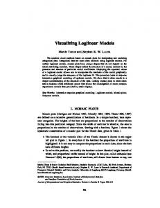
Example Log-linear modelling was used to fit normal (fixed spread), normal (proportional spread), gamma and lognormal selection curves (Table 1) to Fraser River sockeye salmon data (Table 2). The latter three selection curves observe geometrical similarity. Each selection curve was fitted twice, first under the assumption of equal fishing power of the gillnets and then again assuming fishing power to be proportional to mesh size (Table 3, Fig. 1). Each mesh size was fished with equal effort and hence fishing power is the same as fishing intensity in this example. For both normal selection curve models (fixed and proportional spread) the model deviance was lower (indicating a better fit) under the assumption of equal fishing power of the different sized meshes (Table 3). The model deviances from the gamma and lognormal

0 4 17 95 199 202 133 52 25 15 5

selection curve models were not influenced by the fishing power assumption. Overall, the lognormal selection curve provided the best fit. However, the model deviance of 704.3 on 75 d.f. does indicate overdispersion and/ or severe lack of fit. A plot of deviance residuals (McCullagh and Nelder, 1989) shows that there is indeed lack of fit (Fig. 2). These deviance residuals are precisely the same for both the equal fishing intensity and proportional fishing intensity fits of the lognormal shaped selection curve. The residual plot reveals some curious features of these data. It appears that the fishing powers of the smallest (13.5 cm) and largest (19.0 cm) meshes are greater than modelled because of the predominance of positive residuals. Also, for these two meshes the biggest (positive) residuals are for catches of the smaller and larger length classes, suggesting that they caught substantially higher than expected catches of these sizes of

474

R. B. Millar and R. Holst salmon. The converse appears to apply for the other six mesh sizes, with less of the smaller and larger length classes caught than expected.

Normal (fixed spread)

1 0.8

Discussion

0.6 0.4 0.2 0 40

50

60

70

80

90

100

50

60

70

80

90

100

50

60

70

80

90

100

1

Normal

0.8 0.6 0.4 0.2 0 40 1

Gamma

0.8 0.6 0.4 0.2 0 40 1

Lognormal

0.8 0.6 0.4

The approach of Holt cannot use the full set of catch data (Table 2) because it calculates ratios of catches across pairs of gillnets and to avoid highly variable (or non-existent) ratios it is necessary to exclude counts that are not considered sufficiently large (Holt, 1963, p. 108). In contrast, the analysis presented above does use the full data because the likelihood obtained from Equation (1) is appropriate to count data and hence is valid for small or zero catches. With no prior assumptions on the population length distribution the length class variable is fitted as a factor and the model is then equivalent (McCullagh and Nelder, 1989, p. 209) to the SELECT (Share Each Length’s Catch Total) model of selectivity (Millar, 1992; Millar and Walsh, 1992). When a population length distribution is assumed the general model may reduce to the log-linear form in some circumstances. For example, assuming a normal population length distribution and normal shaped selection with proportional spread, the log-linear form is attained (Appendix A). For the Fraser River data this resulted in a population length distribution with an estimated mean length of 60.5 cm and standard deviation of 4.5 cm. The model deviance was 987.3 on 83 d.f. In comparison to the model with no assumed length distribution this is an increase in deviance of 214.5 on a difference of 8 d.f. Notwithstanding the lack of fit noted in the previous section, this suggests that the assumed normal shaped length distribution is not appropriate. In many populations the mixture of different yearclasses of recruited fish will result in a bimodal or multimodal length distribution curve. The genera l model does not reduce to the log-linear form in these cases. However, some statistical software have implemented recently developed smoothing techniques (Hastie and Tibshirani, 1990; Chambers and Hastie, 1992) which enable the user to specify that the population length distribution be a ‘‘smooth function’’ of length without the need to specify a parametric form (Appendix B). The model does not reduce to the log-linear form if the selection curve is of the bimodal form that results from a combination of two selection mechansims

0.2 0 40

50

60

70 80 Length (cm)

90

100

Figure 1. The selection curves (Table 3) fitted to the Fraser River sockeye salmon data. These curves assume equal fishing power of the gillnets – the curves obtained assuming fishing power proportional to mesh size are virtually indistinguishable from these.

Estimation of gillnet and hook selectivity

475

Table 3. Log-linear fits to the data of Table 2. The model deviance is the likelihood ratio goodness of fit statistic and it has 75 degrees of freedom for each of the models shown. Fishing power O mesh-size

Equal fishing powers Model Normal: fixed spread spread O mj Gamma: spread O mj Lognormal: spread O mj

Parameters

Model deviance

Parameters

Model deviance

(k, ó)=(4.044, 5.148) (k1, k2)=(4.095, 0.1035)

862.9 772.8

(k, ó)=(4.072, 5.180) (k1, k2)=(4.120, 0.1029)

883.6 773.2

(á, k)=(158.3, 0.02592)

719.3

(á, k)=(157.3, 0.02592)

719.3

(ì1, ó)=(4.012, 0.0803)

704.3

(ì1, ó)=(4.006, 0.0803)

704.3

19

Mesh size (cm)

18 17 16 15 14 13

55

60

65

70

Length (cm) Figure 2. Deviance residual plot for the lognormal selection curve fits (Table 3) to Fraser River sockeye salmon data. Solid and open octagons represent positive and negative residuals respectively. The area of the octagon is proportional to the square of the residual.

(Hamley, 1975) such as wedging and tangling. Also, the fixed spread gamma selection curves specified by Kirkwood and Walker (1986) cannot be put in log-linear form because the scale parameter â (see Equation 7 on p. 693 of Kirkwood and Walker, 1986) cannot be expressed in the form kf(m). Here k is a parameter to be estimated and f(m) denotes a function of mesh size, m. In these cases the researcher will need to develop customized software to fit the curves using the likelihood derived from Equation (1). Direct experiments of Hamley and Regier (1973) and Borgstrøm (1989) provide strong evidence of increased fishing power with mesh size in their studies (see also Hamley, 1975). If the relationship between mesh size and fishing power is assumed known then it can be included in the log-linear model (Appendix A) through the use of offsets (McCullagh and Nelder, 1989). Otherwise, it can be estimated within the general framework of the model presented here.

This present work is not intended to be a complete analysis of the Fraser River data, but rather to show how indirect estimation from gillnet catch data should proceed and the possibilities for exploration that already exist using existing statistical software. Future research will explore the possibilities and limitations of this general methodology and its ability to make inference associated with gillnet selectivity, including questions about relative fishing powers, population length distributions and shapes of selection curves. One known limitation of indirect estimation is that two different models may give precisely the same fit (Millar, 1995). Therefore, it can never be established that a particular selection curve is the ‘‘right one’’. The inability to distinguish models occurred in the current analysis – fits of gamma or lognormal selection curves do not change when the fishing powers of the gillnets are assumed proportional to mesh size because the offset is confounded with parameters already in the model. Thus, the

476

R. B. Millar and R. Holst

researcher must make a decision concerning the relative fishing powers of the gillnets if fitting gamma or log-normal selection curves. The data cannot do it for her.

References Baranov, F. I. 1948. Theory and assessment of fishing gear. In Theory of fishing with gillnets. Chap. 7. Pishchepromizdat, Moscow. (Translation from Russian by Ontario Dept of Lands, Maple, Ont., 45 pp.) Becker, R. A., Chambers, J. M., and Wilks, A. R. 1988. The new S language. Wadsworth and Brooks/Cole. 702 pp. Borgstrøm, R. 1989. Direct estimation of gill-net selectivity for roach (Rutilus rutilus (L.)) in a small lake. Fisheries Research, 7: 289–298. Boy, V., and Crivelli, A. J. 1988. Simultaneous determination of gillnet selectivity and population age-class distribution for two cyprinids. Fisheries Research, 6: 337–345. Chambers, J. M., and Hastie, T. J. 1992. Statistical models in S. Wadsworth and Brooks/Cole. 608 pp. Feller, W. 1968. An introduction to probability theory and its applications. Vol. I, 3rd edit. Wiley, New York. Gulland, J. A. 1983. Fish stock assessment. A manual of basic methods. FAO/Wiley series on food and agriculture, Vol. 1. Hamley, J. M. 1975. Review of gillnet selectivity. Journal of the Fisheries Research Board of Canada, 32: 1943–1969. Hamley, J. M., and Regier, H. A. 1973. Direct estimates of gillnet selectivity to walleye (Stizostedion vitreum vitreum). Journal of the Fisheries Research Board of Canada, 30: 817–830. Hastie, T. J., and Tibshirani, R. J. 1990. Generalized additive models. Chapman and Hall, London. 335 pp. Helser, T. E., Condrey, R. E., and Geaghan, J. P. 1991. A new method of estimating gillnet selectivity, with an example for spotted seatrout, Cynocion nebulosus. Canadian Journal of Fisheries and Aquatic Sciences, 48: 487–492. Helser, T. E., Geaghan, J. P., and Condrey, R. E. 1994. Estimating size composition and associated variances of a fish population from gillnet selectivity, with an example for spotted seatrout Cynoscion nebulosus. Fisheries Research, 19: 65–86. Henderson, B. A., and Wong, J. L. 1991. A method for estimating gillnet selectivity of walleye (Stizostedion vitreum vitreum) in multimesh multifilament gill nets in Lake Erie, and its application. Canadian Journal of Fisheries and Aquatic Science, 48: 2420–2428. Holst, R., and Moth-Poulsen, T. 1995. Numerical recipes and statistical methods for gillnet selectivity. ICES CM 1995B/:18, 22 pp. Holt, S. J. 1963. A method for determining gear selectivity and its application. ICNAF Special Publication, 5: 106–115. Kirkwood, G. P., and Walker, T. I. 1986. Gill net mesh selectivities for Gummy Shark, Mustelus antarcticus Gu¨nther, taken in south-eastern Australian waters. Australian Journal of Marine and Freshwater Research, 37: 689–697. McCullagh, P., and Nelder, J. A. 1989. Generalized linear models, 2nd edit. Chapman and Hall, London. 511 pp. Millar, R. B. 1992. Estimating the size-selectivity of fishing gear by conditioning on the total catch. Journal of the American Statistical Association, 87: 962–968. Millar, R. B., and Walsh, S. J. 1992. Analysis of trawl selectivity studies with an application to trouser trawls. Fisheries Research, 13: 205–220.

Millar, R. B. 1995. The functional form of hook and gillnet selection curves can not be determined from comparative catch data alone. Canadian Journal of Fisheries and Aquatic Science, 52: 883–891. Myers, R. A., and Hoenig, J. M. In press. Estimates of gear selectivity from multiple tagging experiments. Canadian Journal of Fisheries and Aquatic Science. Regier, H. A., and Robson, D. S. 1966. Selectivity of gillnets, especially to lake whitefish. Journal of the Fisheries Research Board of Canada, 23: 423–454. SAS Institute Inc. 1988. SAS/STAT User’s guide, release 6.03 Edition. SAS Institute Inc. Cary, NC. 1028 pp. Wileman, D. A., Ferro, R. S. T., Fonteyne, R., and Millar, R. B. 1996. Manual of methods of measuring the selectivity of towed fishing gears. ICES Cooperative Research Report. No. 215, Copenhagen. 126 pp.

Appendix A By way of example, if the selection curves are assumed to be normal shaped then

If geometric similarity is assumed then the spread of gillnet j, ój, is proportional to the mesh size, mj. A convenient parameterization is ìj =k1·mj and ó2j =k2·m2j,

(3)

where parameters k1 and k2 are to be estimated. Then,

where

and xLj =L/mj. If no form of the population length distribution is assumed then log(ëL) is fitted as a factor. In doing so, the constant â0 becomes redundant as it is confounded with the overall level of the log(ëL) factor. If, in addition, equal relative fishing intensities are assumed then the log(pj) terms can be ignored and the model is given by Equation (2) in the text. Estimates of k1 and k2 are derived from the fitted estimates of â1 and â2. In this case â1 =k1/k2

Estimation of gillnet and hook selectivity and â2 = "1/2k2, and hence k2 = "1/2â2 and k="â1/ 2â2. If it is assumed that the fishing intensities are proportional to mesh size then (to within a constant that can be ignored), log(pj)=log(mj) and the model becomes log(vLj)=log(mj)+factor(L)+â1 · xLj +â2 · x2Lj which is fitted by treating log(mj) as an offset (Appendix B). In some cases the log-linear form will also result from models where a population length distribution is assumed. For example, if the population length distribution is assumed to be normal with mean è and variance ô2 then

In this case,

477

var1