roughness and zero frequencies in order to equate scores from different tests. Attention is given to .... in (1) is a linear function of the log Pi (although the normalizing constant, a, in. (6) makes the ...... (m ~)3/2 (i.12 ,^#)3/2. Z 3 = ,. (57) ... basic-skills test is given in Table 1. There are 19 ...... sis: Theory and Practice. Cambridge ...
Journal of Educational and Behavioral Statistics Summer 2000, Vol. 25, No. 2, pp. 133-183
Univariate and Bivariate Loglinear Models for Discrete Test Score Distributions Paul W. Holland University o f California, Berkeley
Dorothy T. Thayer Educational Testing Service
Keywords: histograms, data smoothing, test equating, goodness-of-fit diagnostics The well-developed theory of exponential families of distributions is applied to the problem of fitting the univariate histograms and discrete bivariate frequency distributions that often arise in the analysis of test scores. These models are powerful tools for many forms of parametric data smoothing and are particularly well-suited to problems in which there is little or no theory to guide a choice of probability models, e.g., smoothing a distribution to eliminate roughness and zero frequencies in order to equate scores from different tests. Attention is given to efficient computation of the maximum likelihood estimates of the parameters using Newton's Method and to computationally efficient methods for obtaining the asymptotic standard errors of the fitted frequencies and proportions. We discuss tools that can be used to diagnose the quality of the fitted frequencies for both the univariate and the bivariate cases. Five examples, using real data, are used to illustrate the methods of this paper
Discrete univariate and bivariate distributions of test scores occur in a variety of ways throughout the many uses of tests and assessments. It is rare that these empirical distributions follow any of the familiar classical discrete distributions such as the binomial, hypergeometric, or beta-binomial (also called the negative hypergeometric, Keats & Lord, 1962), even though these classical forms are sometimes very useful for special purposes (Lord & Novick, 1968). This paper discusses the general class of exponential families of discrete distributions, which we simply refer to as loglinear models, that are appropriate for fitting a wide variety of discrete empirical distributions. This is an enormous and flexible class of models for score data that can be used to give good fits to real test score data with a relatively small number of parameters. We consider both the univariate and bivariate cases, and discuss diagnostic tools that can be used to assess the fit of these models. The material discussed here has applications far beyond those of educational testing and assessment, but we will concentrate on and give most of our examples from educational test applications because they often exhibit a variety of problematic properties that can be easily handled by the models we discuss. In the univariate case some of these problems are: (a) the range of possible 133
Holland and Thayer score values is not just the non-negative integers, 0, I, . . . T, but can be any finite set of values, x~, x2 . . . , x r that may include both positive or negative values; (b) moments beyond the second may be needed to adequately describe the data; (c) the pattern of the frequencies can be skewed, u-shaped or have multiple modes; (d) the frequencies can exhibit regular "teeth" that are not due to sampling error; (e) individual frequencies can substantially depart from the smoother pattern that the other frequencies exhibit; (f) and more generally, different types of models might be needed to fit the frequencies from different parts of the score scale. In the bivariate case the situation can be even more complex with some of the above problems occurring for one variable and others for the other variable. The models described here are purely empirical in the sense that their parameters and forms do not necessarily have simple interpretations in terms of underlying structures such as latent proficiencies or "true scores." This fact is often true of Ioglinear models for other discrete multivariate distributions, although not always (see Cressie & Holland, 1983; Tjur, 1982; Clogg & Goodman, 1984). In fact, because these are exponential families of models, they are often most usefully described in terms of their sufficient statistics (or sample "moments") rather than their "natural" or exponential parameters because, for exponential families of distributions, maximum likelihood estimation corresponds exactly to estimation based on the "method of moments" whereby the sample moments that correspond to the sufficient statistics are fit perfectly by the corresponding fitted moments of the model (see Lehmann, 1986; Rao, 1965; Barndorff-Nielsen, 1978). The models described here are useful for purposes that involve the raw test-score data--such as histogram smoothing, or preliminary fitting for use in subsequent procedures such as test equating (Holland & Thayer, 1989; Holland, King, & Thayer, 1989; Kolen & Brennan, 1995). While the classical models for discrete distributions can have from one to four parameters, from the binomial with one parameter to the four-parameter beta-binomial (Lord, 1965; Little & Rubin, 1994), our experience suggests that univariate score distributions may need more than four parameters to describe them adequately--see Hanson (1996) for more examples of this. More complex data may require considerably more parameters (see the examples in Section 5) but, of course, sample size plays an important role here. Little in this paper is original, except for one of the computational formulas for the standard errors in Theorem 2 of Section 3 and possibly some of our suggestions for diagnosing the fit of these models in Section 4. Our goal is to publicize loglinear models for score distributions to a wide audience who may often encounter score distributions, to organize some useful results about them, and to describe how to assess their fit to real data in one place. Related discussions can be found in Agresti (1984, 1990), Bishop, Fienberg, and Holland (1975), Darroch and Ratcliff (1972), Haberman (1974a, 1974b, 1978), Hanson
134
\
\
\ \
Univariate and Bivariate Loglinear Models
(1996), and Rosenbaum and Thayer (1987). Much of the technical material in this paper was originally brought together in an ETS report, written by Holland and Thayer (1987). The rest of the paper is organized as follows. In Section I, we describe the general class of models of interest to us and then, in Section 2 give some examples and relate them to various classical models where possible. Section 3 is devoted to maximum likelihood estimation for these models, discussing Newton's Method, starting values, and convergence criteria. In Section 3 we also indicate efficient computations for asymptotic standard errors and confidence intervals and in Section 4 we discuss various diagnostic tools for assessing the fit of these models for both univariate and bivariate distributions of scores. Section 5 illustrates the discussion with five examples that include test-scores and other distributional data.
1. Loglinear Models for Score Distributions We begin with a general description of the models and then discuss some specific examples. First of all, let n denote a (column) vector of cell frequencies with entries, nl, n 2. . . . , n T, so that T denotes the total number of "cells" in the histogram or bivariate distribution, in the univariate case, T is the number of possible values of the random variable, whereas in the bivariate case, T is (usually) the product of the number of possible values for the two random variables--but in the last "triangular" example of Section 5 it is not. Associated with each cell there may be one or more numerical values which we will call "cell values." Cell values are the "possible values" for random variables with a discrete distribution. We will ignore the cell values until Section 2 because they play no essential role until we examine specific examples. If the data are arranged in a two-way array (i.e., a bivariate distribution) then we regard it as a vector by stacking the columns of the array on top of each other starting with the first column on top. More complex examples, i.e., triangular or other incomplete arrays, are likewise put into a single vector form by similar conventions. The particular convention used in any case only affects the form of the B-matrix and u-vector discussed below. We give examples of these in Section 3. The total number of cases is N ~ n i , and the frequencies themselves are i non-negative integers, n i > 0, some of which could be zero. If we regard the data in a univariate or bivariate frequency distribution as a sample of N independent observations of a discrete random variable (or, equivalently, a random sample from an infinite population of discrete values), then we may make the distributional assumption that n has the multinomial distribution, M(N,p), where p denotes the (column) T-vector of population cell probabilities, Pa, P2 . . . . . Pr, corresponding to the cell frequencies nt, n z . . . . . nr, and we assume that Pi > 0 and ~ Pi |" =
:
i
135
Holland and Thayer
This assumption will be satisfied in those cases where it is reasonable to regard the data as a sample from a larger population for which each possible value is, indeed, "possible" if not actually observed. Sometimes, for example, when the data represent the entire population of test takers of a given test, the data are a population rather than a sample from one. In such cases, it may still be useful to use these models, for example, to smooth out inessential irregularities in the pattern of the frequencies in order to focus on their main features. In many testing applications the actual population is not well specified. Under the assumption of a multinomial distribution, the probability of the cell frequencies, i.e., the data, n I, n 2. . . . . nT, is proportional to I-I P'/~; hence, taking i
logs, we see that the log-likelihood function for this problem is L=
~n ilogpi.
(1)
i
It is well-known and easy to show the mean vector and covariance matrix of the M(N, p)-distributed vector, n, are E(n) = Np
(2)
Coy(n) = N(Dp - pp'),
(3)
and
where Dp denotes the diagonal matrix based on the vector p and pt denotes the vector transpose o f p (Bishop et al., 1975). It is convenient to have a single notation for the expected value of n, so we denote it by m, i.e., m = N p . In terms of m and N, Cov(n) may be expressed as (4)
Cov(n) = D m - N - 1 m i n t = Y'm"
The covariance matrix in (4) occurs sufficiently often in this paper to deserve its own notation, Zm. In this notation, the vector m on which ~Z is based, must have non-negative elements that sum to N; this fact is used later on in equation (37).
Definition o f Loglinear Models
:
The vector p satisfies a loglinear model if the multinomial parameters, {Pl}, have the form log P i
= a + U, + bi13,
(5)
where: log denotes logarithm to the base e; u i is a known constant for each i; b i is a (row) K-vector of known constants for each i; and 13 is a (column) K-vector of K free parameters. The values {u,} are used to specify the "null" distribution to which the Ioglinear model reduces when the parameter 13 is set to zero. When 13 = 0 the pi are proportionalrto exp(u~), where exp(x) denotes the exponential function e x. The term a is the "normalizing constant" that makes the s u m o f the p~ equal to i. Hence, solving for a in terms of I~ yields: 136
Univariate and Bivariate Loglinear Models
et = (x(13) = - l o g ( ~ exp(uj + Oil3)). J
(6)
Loglinear models defined in the log-p scale in (5) can also be expressed in the p-scale (where c~ disappears) as: exp (u i + bi13)
(7)
P i ' = Eexp(uj + b~13) ' J
The Likelihood Function for Loglinear Models
.
An important rationale for using the Iog-p scale is that the likelihood function in (1) is a linear function of the log Pi (although the normalizing constant, a, in (6) makes the likelihood function non-linear in 13). If the Ioglinear model for Pi in (5) is substituted into the likelihood function in (1) we find that: L = Z n i ( o t + u i ']- bi13) = o N i
-~- E niui + Zrlibi13 i i
(8)
or
L = a N + E n i u i + Z (Enibik)fSk, i
k
(9)
i
and hence the sufficient statistics for such a model can be read off the loglikelihood function as the K coefficients of the components of 13 and they are the "generalized sample moments": S k = ~nibik, for k = I to K,
(10).
i
where b~ is the kth component of the (row) v e c t o r b i. Maximum Likelihood and Moment Matching "Moment matching" will play an important role in this discussion and it always takes the following form. Parameters estimated by maximum likelihood are such that the sample moments that comprise the sufficient statistics of the model are equated to their expected values under the model. This means that E(S,) = Sk,
(11)
~ r h i b i k = ~nibik or ~fiibik = ~,(ni/N)bik for k = 1 to K, i. i i i
(12)
or equivalently that
where r~i and /~/ denote the fitted or estimated values of m i and Pi under the model. We note that if p satisfies a Ioglinear model, then m will satisfy the same model with a replaced by ot + log N. 137
Holland and Thayer In matrix notation, a loglinear model for p (or m) can be expressed as log(p) = a + u +B[3
(13)
where: log(p) denotes the (column) T-vector whose coordinates are the natural logarithms of the coordinates of p; ot is the normalizing constant specified in (6); u is the (column) T-vector of known constants, u i, in (5); B is the T by K matrix of known constants of rank K formed by arranging the row vectors, b;, one on top of the other; and [3 is a (column) K-vector of free parameters---called the "natural" or exponential parameters of the model. A fundamental restriction is that K < T 5o that there are fewer parameters in [3 than there are degrees of freedom in p. The T by K B-matrix is analogous to the design matrix or "X-matrix" of multiple regression. It is used to specify loglinear models in the same way that the design matrix is used to specify linear models in regression.
The Role of the u-Vector As mentioned earlier, the role of u in (13) is to specify a "null" distribution for the exponential family that holds when the parameter [3 = 0, i.e., the null model. Any loglinear model can be thought of as centered on its "null distribution." For example, if u = 0, then from (7) we see that the null distribution is the discrete uniform distribution over the set of possible cells or categories. In the next section we show that for the binomial distribution the choice of u :~ 0 and the null distribution for the binomial is not the uniform distribution.
Equivalent Loglinear Models It is easy to see from (7) that if each u i is changed to u i + c for some constant c then the loglinear model is unchanged. Similarly, if the rows of the B-matrix are changed to biA+c, and the parameter [3 replaced by the new parameter A - t[3, where A is a non-singular K by K matrix and c is a (row) K-vector, then the loglinear model for p is unchanged. These transformations are useful for specifying alternative equivalent forms of a given Ioglinear model. Examples of equivalent toglinear models that have u-vectors or B-matrices that differ by the transformations indicated above are given in the next section.
2. Some Cases of Loglinear Models Discrete distributions have two components---cell-probabilities and cellvalues. In the univariate case each cell has a single cell-value associated with it. In the bivariate case there are two cell-values associated with each cell, one for each variable. In this paper the cell-values are regarded as given by the nature of the data, and are not quantities to be estimated. So far, the cell-values of the distribution have played no role. They do influence the choice of the [3-matrix and the u-vector in (13) and we illustrate them in several cases in this section. A loglinear model for p is linear in the unknown parameter, [3, when p is expressed in the log-scale. The model is specified by the known "null model" vector u and the known "design" matrix B that specifies the sample and 138
Univariate and Bivariate Loglinear Models
population moments that, along with u, uniquely describes the Ioglinear model. In this section we discuss various e x a m p l e s of these models and the types of flexibility they can exhibit. C a s e A: The Discrete U n i f o r m D i s t r i b u t i o n
Set u = 0, B = anything, [3 = 0. From (7), for this case, we have
1
(14)
Pi = ,~.
In the univariate case, the cell-values for the uniform distribution could be any set of T distinct values, x~, x2, . . . , x T, and in the bivariate case, any set of T discrete pairs of values, (xi,y.i). From our c o m m e n t s earlier about the effect of transforming the u-vector, we see that the condition u = 0 could be replaced by u = c for any constant, c, and the result would still be the uniform distribution over the set of cell-values. Case B: The B i n o m i a l Distribution, B(C, rr), the N u m b e r o f S u c c e s s e s in C Trials with S u c c e s s P r o b a b i l i t y rr
In this case the cell-values associated with the cells of the distribution are the non-negative integers, 0, I . . . . C, so we let: T=C+I;
xi=i -
K = l; I3 and we set u~ = log
1, f o r / =
I to T;
b i = (Xl), for i = 1 to T;
= (/3);
[(c)] xi
, where
C)
Xi
denotes the binomial coefficient,
"C
choose Xi". Inserting these values into (7) yields the familiar formula for the binomial Pi:
Pi =
(C) xi
7rX; (1 - 'rr)C-x;,
(15)
where 7r = et3/(l + et3). This is the B(C, -n') distribution. The sufficient statistic from (10) is given by, S I = ~nibil = ~nix i = ~ni(ii
i
1) = ~ i n i - N.
i
(16)
i
To obtain the usual form of the sufficient statistic for the B(C, rr) distribution, instead of settling x; = i - 1, we use the linear transformation, new b i = N - I b i + N - I , 139
Holland and Thayer to obtain an equivalent Ioglinear model where S I becomes the sample mean, ~i(n~/N), which is the usual form of the sufficient statistic for the binomial i
parameter, "rr.
Case C: Models that Involve Both the Mean and the Variance The flexibility of the binomial distribution just discussed is limited to fitting only the mean of the distribution of the data. The higher moments of the resulting fitted distribution are then determined by this estimated mean value. For many problems this will not produce a satisfactory fit to the data and various models have been proposed for accommodating "over" and "under" dispersion in the binomial case (see Breslow, 1984; Dean, 1992; Efron, 1986). For example, if 'rr in (15) is given a prior distribution (such as the beta distribution), then the resulting "compound binomial distribution" will have a variance that is larger than that of the binomial distribution with the same mean value. Similarly, if instead of assuming a common value of "rr across all C trials, we let the values of "rri be different on each trial, the resulting distribution has a variance that is smaller than that of the binomial distribution with the same mean value. These models can be used to fit distributions on 0, 1. . . . C, that have variances that are not the same as that of the binomial distribution with the same mean value as the data, N/~ = Y f i ( n i / N ). i
Within the families of distributions that we are considering here it is a straight-forward matter to specify a variety of models that can fit means, variances and other moments of the data distribution exactly. These models generally give fits that are clearly better than simpler ones. For example, consider the loglinear model l o g p i = o. + u i + xi~ t + x~[32.
(17)
In this case, b i = (x i, x~) and ~ ' = (13 I, 1132).Regardless of the choice of the u i, and the values of the xi, the sufficient statistics for this model are ~ x i n i , and ~x2ini, i
i
which are linear transformations of the first two sample moments, ~ and ~
x2(ni/N).
xi(ni/N )
i
The
"moment-matching" property of maximum likelihood
i
estimation for exponential families in (12) means that the maximum likelihood estimates, (13~,132), will force the estimated probabilities, Ifiil, to satisfy these two moment-matching conditions:
Z xi i = Z x,(ni/N), i
X
=X
i
i
(18)
These two moment-matching equations are equivalent to forcing the mean and variance of the data to be fit exactly by the mean and variance of the distribution specified by the cell-values and the fitted proportions,/3~. 140
Univariate a n d Bivariate Loglinear Models
If u; and x i have the values given for the binomial distribution in Case B, then the distribution in (17) is a generalization of the binomial distribution (i.e., it is exactly the binomial when 13l = 0). It can fit data that have either under- or over-dispersion for otherwise binomial-like data. If, on the other hand, u i = 0, then (17) corresponds to a different 2-parameter family of distributions that does not contain the binomial as a special case. It also exactly fits the mean and variance of the sample. Neither of these models corresponds exactly to the variations on the binomial distribution mentioned at the beginning of this example, and for data-smoothing purposes they may be regarded as competitors to these models. Of course they are more flexible than models like the compound binomial because they are not restricted to being over-dispersed relative to the binomial with the same mean value, and the cell-values, x~, can be any set of numbers, not just non-negative integers. In addition, as we shall see in the examples of Section 5, we can add higher moments than the second moment to the list of sufficient statistics and obtain models with more parameters that can fit more complicated data distributions.
Case D: Other Univariate Moments The ath "power moment" of the population and of the sample are, respectively,
x~ p i and ~ x~ (hi~N). i
(19)
i
Such sample moments will be the sufficient statistics for a loglinear model if the corresponding powers of x i are included in the model, as illustrated for the case of a = I and 2 in (17). The power moments are useful because of the general familiarity of distributional measures based on the first four moments, i.e., mean, variance, skewness, and kurtosis. In our experience, we have often found it necessary to include power moments as high as five or six to obtain good fits to univariate data distributions, although this clearly depends on several factors including the sample size, N. Loglinear models that use the power moments are sometimes called polynomial loglinear models, Hanson (1996). However, the power moments are not the only ones that have utility in fitting univariate distributions. A very useful class of alternative moments are the "subset moments" defined as follows. A subset, S, of cells is identified, and the indicator function for S, Is(i), is used to define the "subset moment for S,"
~', Pi = ~ Is(i)pi,
iES
i
(20)
where Is(i) = 1 if i E S, and Is(i) = 0, otherwise. Subset moments have several uses. For example, if the frequency for one cell of a histogram does not seem to follow the pattern of those for the other cells then it is often useful to isolate that cell so that it does not distort the fit for the remaining ones. Thus, if cell 1 is the problematic one, then S = {1}, a n d / c ~ l ( i ) = 0 for all i except i = 1. In (17) this 141
Holland and Thayer could be accomplished by using the model I o g p i = a + u i + xi[31 -[- x~[32 q-
/{11 (i)[33'
(21)
In this case, b i = (xi, x,2., Ill ~ (i)), [3'= (13 I, [32, [33) and u i could be any of the choices discussed previously. Another use for subset moments is to fit one set of power moments to one part of the data and another set of power moments to another part of the data. This could be clone by using a model of the form log Pi = e~ + u i + xi[31 + x~ ~52 + Is(i)[33 + xils(i)[~ 4.
(22)
In this case, bi = (xi, xZi, Is(i), xi Is(i)), [3' = ([31, [32, [33, [34) and ui could be any of the choices discussed previously. The model in (22) will match the first two moments of the cell values for the entire distribution, the total frequency in the cells denoted by S, and the mean of the cell values for the cells in S. This is very useful when the cells indexed by S are different in systematic ways from the others as happens when the frequencies exhibit non-random features like "teeth" spaced at regular intervals along the score scale.
Case E: Models f o r Discrete Bivariate Distributions A bivariate distribution of test scores will consist of a doubly indexed set of f r e q u e n c i e s , f = {fo}, plus a set of cell-values for the scores corresponding to the rows, {xi}, and another set of cell-values for the scores corresponding to the columns, [ yj}. The value o f f : i is the number of cases in the sample where the row score is xi, and the column score is yj. The various (power) moments of this bivariate distribution can be expressed as linear combinations of the frequencies, e.g., x~' y~ ( f i N ) .
(23)
I,J
When b = 0, this is the ath moment of the distribution of the row scores, and if a = 0, this is the bth moment of the distribution of the column scores. When a and b are both positive, these are the cross moments of the joint distribution of the row and column scores, e.g., a = b = I is the cross moment related to the covariance and correlation between the two scores. Associated with the frequencies are the population cell-probabilities, {Pij}. Loglinear models for the cell-probabilities may be specified in a manner that is similar to (17) for the univariate case, for example, log PO = a + uij -k- xi[3x I + X~[3x2
"[- Yi[3yl + Y~[3y2 + xiYi[3xyll"
(24)
In this case, [3' = ([3xl, 13.,-z, [3yl, [3yZ, [3.,yl0. It is harder to describe the elements of the B-matrix since it must reflect the stacking of the columns o f f on top of each other. If the subscript "j(i)" denotes the ith row of t h e j t h column o f f , then 142
Univariate and Bivariate Loglinear Models let bj~ij denote the row of the B-matrix corresponding to the ith row of the jth column o f f . We can then express bjm as:
bjli) = (x,, xZi, yj, y~, xiYj).
(25)
The five-parameter model in (24) is an analog of the bivariate Normal distribution and it has the same sufficient statistics--the sample means, variances and the covariance. Each choice of "null distribution", u, in (24) results in a different model with these sufficient statistics. We have found that in many applications satisfactory fits to data occur when we choose u = 0, even though this does not result in a generalization of the binomial distribution. In the special case wherex i = i I,fori=l toC+ I,and))=j1 f o r j = l t o D + l, i f w e set u o equal to u 0 = log
xi
YJ
,
(26)
then (24) reduces to two independent binomial variates, B(C, ~t) and B(D, -rr2), when 13.,.2, 13y2, and 13.~vlt all equal zero. Hence, (24) can be used to give a generalization of two independent binomial variates. However, it ought to be pointed out that, in general, the marginal distributions of (24) are not binomial distributions--this failure of "marginal inheritance" is typical of exponential families of distributions (see Barndorff-Nielsen, 1978). As mentioned earlier, we have often found it necessary io include powers as high as five or six to adequately fit the univariate margins of bivariate distributions. However, our experience also suggests that for many problems the joint distribution is adequately represented by models that include as sufficient statistics the cross-moments of the form (23) with a, b < 2. In the bivariate case there are three classes of parameters/moments that arise: those that are only associated with the row score (x~), e.g., 13.,.~ and 13.,.2; those that are only associated with the column score (yj), e.g., ~yl and 13y2; and those that are associated with both, e.g., 13.,~q~. Because unusual features of the marginal distributions often propagate into the cells of the bivariate distribution, it is important to consider all three types of parameters when examining the fit of a model (we discuss this further in Section 4. As with univariate distributions, it is sometimes, helpful to use subset.moments as well as power moments to adequately describe bivariate distributions. In the bivariate case, row and column totals are examples of subset moments. These can also be used to create models with row and column "effects" as discussed in Rosenbaum and Thayer (I 987). In such models, there is no smoothing of the row or column distributions and we have found that for many applications to test score distributions it is important to smooth the observed marginal distributions. This is why we concentrate on such "smoother" models in the examples of this paper. In the bivariate case, subset moments also can be used 'to define the sums of the upper and lower off-diagonal cells of the array. 143
Holland and Thayer This forces a match of the total cell frequency in these areas of the bivariate region with that of the fitted cell frequencies, ~i./, for that region.
Case F: Square Triangular Arrays Triangular bivariate distributions are examples of distributions with structural zeros (Bishop et al., 1975; Holland & Wang, 1987). They can arise when certain combinations of values for the two variables, X and Y, are impossible. Although there are many ways these can arise in real data, we will consider only the "square" case in which the two variables have the same number of possible values, C. (However, by manipulating the B-matrix appropriately any type of incomplete array can be handled in a manner similar to what we do here.) One way the square case can arise with score data is when the scores are "before and after" ratings with the special property that the ratings can only stay the same or improve over time. This will result in the initial rating X always being less than or equal to the subsequent rating, Y. If we array the frequencies, {f/j}, as a two-way square array, and if the cell values are xi = i, i = I to C, and yj =j, j = 1 to C, then necessarily the frequencies, f:/for i > j will be equal to zero since it is impossible for X to exceed Y. This results in a triangular array in which the lower-left triangle-half of the array is all zeros and the only place where non-zero cells can occur is in the upper-right triangle-half of the array. We can express the structure of triangular arrays in much the same way that we express two way arrays, as stacked vectors, but this time of varying length. Again, if we let '~j(i)" be a subscript that denotes the ith row of the jth column of the triangular array, we need only add the restriction, i -->j, to restrict the cells to the upper-right triangular-half of the two-way array. In this way we can specify models for the square triangular array just like the one indicated in (24) except that they are restricted to the upper-right triangular-half of the array. In this case, 13'= (13xl, 13.,.2, [3vl, 13y2, 13xyll). AS in Case E, let bj:i) denote the row of the B-matrix correspondi'ng to the ith row of the jth column o f f with the restriction that i -->j. We can then express bj:i) as before:
bj(i) = (xi, x~, yj, y2, xiYy).
(27)
For any choice of uij, e.g., u U = 0, such a model will produce a fitted distribution that matches the means and variances of the row and column distributions, and the correlation coefficient of the triangular bivariate distribution. (For other discussions of incomplete triangular arrays see Bishop et al., 1975).
3. Maximum Likelihood Estinmtion, Asymptotic Standard Errors and Conf'aience Intervals This section is intended as a summary of several technical issues regarding the implementation of maximum likelihood estimation for the loglinear models described above. 144
Univariate and Bivariate Loglinear Models
Maximum likelihood estimation proceeds by maximizing the likelihood function given in (I). When a loglinear model of the form (5) is substituted for log Pi in (1), L becomes a well-behaved function of [3, L([3) and usually can be maximized by differentiating L and solving the resulting likelihood equations, i.e., by solving OL
--=0 0[3
(28)
for [3. The solution, [~, is the maximum likelihood estimate (role) of [3. We will refer to/;i = p,.(l~) and mi = m/([]) as the roles (or role fitted values) of the cell probabilities and cell frequencies, respectively. Applying well-known results (Lehmann 1983; Barndorff-Nielsen, 1978), the role, [3, is asymptotically Normal with mean [3 and covariance matrix
cov( ) = (
o2L )-, '
0[30[3/
(29)
Hence, to implement maximum likelihood estimation and the corresponding confidence intervals and standard errors for these models we need expressions of the derivative vector and second derivative matrix of L. These are summarized in Theorem I, which we state without proof. (For details see Holland & Thayer, 1987.)
Theorem ]
For the Loglinear Model Specified in (5) or (13)
(a) ~OL= B t ( n - m ) ,
(30)
op
O2L (b) 0130-----~= - (Bt
~mO),
(3 l)
where n is the vector of cell frequencies, m is the vector of fitted cell frequencies satisfying (5), B is the B-matrix of the model, and Zm is the covariance matrix defined in (4). Setting the derivative vector in (30) to zero and simplifying yields the following matrix version of the moment matching equation (12): Btn = Btm.
(32)
In (32) m is a non-linear vector function of the natural parameter [3 and Newton's Method is often used to solve (32) for the role, [~. In this setting it is useful to describe Newton's Method as follows. 145
Holland and Thayer Newton's Method for Obtaining MLEs (a) initialize the iterate, I~(°~, to some starting value, (b) at iteration n, update 13~") by solving the linear system
(B t E , n B ) 8 ( . +
(33)
I) = B i n _ B t m
for ~(,,+l), set [l("+° = 13(") + ~(.+o, and recompute in, Btm and Bt~.mB from the new value of [3("+l)' (c) repeat (b) until a convergence criterion is satisfied. There are two types of computational issues that should be mentioned here. First, the computation of Bt~,,,,B should be done directly rather than forming the potentially huge T by T matrix, ~,,,, and multiplying it by the others. In fairly routine bivariate applications it often occurs that T exceeds 2000, so that Y.,,,, would contain over 4 million entries. It is easy to show that the (r,s)th entry of Bt~,,,B can be computed directly as
~b,rbi.,.m i - N - ' ( ~ b i r m i ) ( ~ j bj.dnj),
(34)
which does not involve forming a large matrix or summing over more than T terms at a time. Similarly, the rth component of Btm is directly computed as: ~birmi .
(35)
i
The second computational issue is solving the system in (33). It can and should be done using standard linear algebra routines that do not require the computation of the inverse of (B~mB) (Dongarra et al., 1979; Searle, 1982). To implement the above version of Newton's Method one needs to specify both a starting solution, [3(°), and a convergence criterion. We have found the following to be useful in this regard for a variety of problems.
Starting Solutions (This is based on a suggestion in Rosenbaum & Thayer, 1987). First set
a i = pni + (1 - o)(N/T),
(36)
where we have often found p = 0.8 to be useful; having the parameter p to vary however, provides a flexible tool for trying to find a satisfactory starting solution for Newton's Method. Equation (36) produces a smoothed set of "frequencies" that are shaped like the {nil have the same sum, N, but are non-zero even if some of the n i = 0. Denote the column vector whose components are the a~ by a. Next, solve the linear system
(Bt]f, aB)[3 (°) = BtY-a [log(a) - u] 146
(37)
Univariate and Bivariate Loglinear Models for 13(o), where, log(a) is the vector whose components are log a r Because the a i are positive and sum to N, X,, in (37) is a legitimate matrix of the form D, - N - laat. The geometric effect of (37) is to project the vector log(a) - u into the linear subspace spanned by the columns of B, and then to recover the corresponding value of 13 that produces this projection of log(a) - u. As long as not too many of the {ni} are zero, we have found the solution to (37) to yield a useful automatic starting solution for Newton's Method in this case. Formula (34), with m replaced by a, can be used as a computationally efficient way of computing the elements of Bt~,aB in (37). Similarly, the rth element of Bt~.,a[Iog(a) - u] in (37) may be directly computed as:
~i bi,.ai[log(ai) - ui] - N-'(~,i birai)(~j aj[Iog(aj) - uj]).
(38)
As in step (b) of Newton's Method, the solution of (37) for 13(o) can be accomplished without inverting the matrix Bt]BaB.
Convergence Criteria There are two basic criteria that can be monitored during this application of Newton's Method. The first is the quantity that is being maximized by the algorithm, the likelihood function, L, in (1). The second concerns the satisfaction of the likelihood or moment matching equations (28), (12) or (32) which must occur when the maximization of L is uniquely determined by its first derivatives being zero. The criterion that the iterate, 13oo, does not change much at each iteration is an indirect check on the progress of the algorithm and may not always be as useful as the two direct checks on the convergence indicated above, although it is clearly related to them through the smooth relationship between L (and m) and 13. Checking the maximization of L proceeds as follows. At the end of the nth iteration of step (b) above compute ot(''+° from 13(,,+1) via formula (6) and then the (n+l)st value of L, L (''+E), via formula (9), which is preferred over (8) since it does not require recomputing the sufficient statistics at each iteration. One natural convergence criterion is to require that the relative change in the log likelihood function be less than some specified value, i.e., that
L(,,+ i) [
_
--L (')
L(n)
< e.
(39)
Checking the approximate satisfaction of the likelihood equations proceeds as follows. At the beginning of the nth iteration of step (b) above compute the relative error made in each fitted moment and require that it be less than some specified value:
Zbi,& -- ~,bik,,,~")[ ~bikn i J< &
(40) 147
Holland and Thayer When the kth sample moment, ~,bikni, is zero, then (40) should be replaced by the absolute value of the kth fitted moment, 2,oiffn ~(,0, to avoid dividing by zero. In the implementation of Newton's Method for this problem we have found that it is often useful to center and scale the column of the B-matrix so that ~
~bik = i
0
-
and ~b/2~ = 1. i
(41)
This tends to give better numerical stability to the algorithm, but it makes it necessary to rescale the mles of [3 to get back into the original scale, if this is of interest. However, for most applications this rescaling of 13 is not important since the natural parameters are usually of much less interest than the fitted moments of the distribution.
Confidence Intervals and Standard Errors We begin with the well-known observation that (29) and (31) together imply that the large sample standard errors of ~ can be approximated by
Coy((3) = (Bt~,,B) -'.
(42)
The K by K matrix in (42) can be used to obtain standard errors for I~ and confidence intervals for [3 using the usual methods. However, these are not usually of much direct interest in many problems because of the general lack of interpretability of the natural parameters in exponential families. But there is often direct interest in standard errors in the fitted values, either/3 i = pi([~) or rh i = mi((3). For example, in our work on test equating (Holland, King, & Thayer, 1989; Holland & Thayer, 1989), it is crucial to obtain an estimate of the full covariance matrix of the fitted values, fi~ = p;(l~), as an intermediate step in the process of finding the "standard error of equating," a measure of the accuracy of the estimated equating function. The mapping of 13 into rh~ = mi(($ ) is differentiable so that the asymptotic (as N---) oo) covariance matrix of th can be formed using the 8-method formula (Bishop et al., 1975). This formula is:
Cov(rh) =
where
(Om) -~
^l/Om'~ t
Cov(~)~-~ ) ,
(43)
denotes the T by K partial derivative matrix of the vector-function
m([3) with respect to ~, Cov(~) is the K by K covariance matrix in (42) and, as usual, the superscript t denotes matrix transpose. It is straightforward (Holland & Thayer, 1987) to show that the partial derivative matrix in (43) is given by
148
Univariate and Bivariate Loglinear Models Combining (43), (42), and (44) reveals the following formula for the covariance matrix of the fitted cell expected values: Cov(rn) = ~,mB(B~,m B) - I B t ] ~ m.
(45)
For the same reasons that it is often computationally more efficient to avoid computing directly with the matrix ~m in (33), formula (45) is not a good way to compute the elements of this covariance matrix. A better way to compute the elements of the matrix in (45) is given in Theorem 2, which is proved in detail in Holland and Thayer (1987).
Theorem 2 In the notation above, Cov(th) = ~,mB(B~mB) - IBt]~ m = CC t
(46)
where C is the T by K matrix formed as follows: (a) C =__Dv7ff Q, where D~,-~ denotes the diagonal matrix .with diagonal entries ~v/mi, and
(b) Q is the "Q" part of the "QR" factorization (Dx/--d- N-'~/--m--m')B = QR ,
(47)
where Q is a T by K matrix with orthogonal columns, and R is a K by K upper triangular matrix. Dongarra et al. (1979) describe an algorithm for computing the QR factorization of a T by K matrix. The entries of the matrix in (47) to be factored can be computed efficiently in a manner similar to the discussion of the matrices occurring in Newton's Method. The (i, k)th coordinate of the matrix on the left-hand-side of (47) is directly computed by
{bik - N-t(~'~bjkmi)}, )
(48)
and once the Q-matrix for the QR factorization of this matrix has been found, the (k, k)th entry of the matrix C in Theorem 2 is obtained as ~/miiqik"
(49)
If confidence intervals are desired for the fitted cell frequencies, mi, then asymmetric, non-negative intervals for them can be obtained by first finding confidence intervals for log(mi), and then exponentiating them to obtain the confidence intervals for mi. This produces asymmetric intervals for the expected cell frequencies that do not contain zero or negative values. The covariance matrix for Iog(th) can be shown to be the matrix in (45) pre- and post-multiplied 149
Holland and Thayer
by the diagonal matrix, D , 2 (Holland & Thayer, 1987). The resulting covariance matrix can be computed in the manner indicated in Theorem 2, with the matrix C defined as C~O
-[ vTffQ
(50)
where Q is the same matrix as in Theorem 2. The obvious analog of (49) can then be used to compute the entries of (50).
4. Tools for Diagnosing the Fit of These Models We take the position that examining the fit of a model is not a simple all-or-none process in which a decision is made that a model either fits or fails to fit the data. Rather, models are adequate in some respects and inadequate in others. The tools we discuss are designed to highlight where these adequacies and inadequacies arise in a given set of data. We begin with the univariate case and then consider the bivariate case. An alternative discussion can be found in Haberman (1974a). The Univariate Case
We think that graphical and tabular displays as well as formal test statistics can help us assess the adequacy of the fit of a distribution. In the univariate case the usual graphical display of the histogram of observed frequencies {hi} with the fitted cell means {Phi} superimposed on it can give a quick visual summary of how well the fitted values track the observed data. It is, of course, well-known that the greatest departures of the data from the fitted cell means will arise where the fitted cell means are the largest because that is where the largest sampling variability is. This occurs in the regions of the modes of the distribution, and can mislead attention away from other places where the fit is in fact relatively worse. To give a better assessment of these discrepancies, we have found the FreemanTukey residuals, +
+
-
(5,)
to be a very useful tool. These residuals are a smoothed version of the usual square-root transformation for Poisson variates, and they are most useful when T and N are reasonably large. If the model fits the data, then these residual are approximately normally distributed with mean 0 variance I. Because of this, it is also helpful to display the residuals in a Normal Probability Plot in which the ordered residuals (as y) are plotted against an x-axis of the expected values of the N(0, l)-order-statistics (Normal Scores). If this plot follows the line of slope I through the origin then this is good evidence that the model fits the data. More formal goodness-of-fit tests are based on the likelihood-ratio-test statistic, or "likelihood-ratio chi-square", or "G 2'' given by: G2 = 2~nilog(ni/~ti)" i
150
(52)
Univariate and Bivariate Loglinear Models
Other goodness of fit chi-square statistics that usually give similar results are the Pearson Chi-square statistic.
x~, = Y~ (hi - *hi)2, i
(53)
r?li
and the Freeman-Tukey Chi-square statistic, X~r = • { V ~ / +
~
+ 1 - V~i
+ 1}2.
(54)
i
If the model is correct, then each of these chi-square statistics has an approximate (for large N) chi-square distribution with T - 1 - K degrees of freedom. Nested models easily arise in this setting. If we fit a two-parameter loglinear model of the form indicated in (17) to some data and then decide to see if the fit can be improved by adding a cubic term in xi to the model, i.e., the t e r m Xi3[~3, then the original two-parameter model is a special case of the larger threeparameter model with linear, quadratic, and cubic terms in x i. The likelihoodratio chi-square statistics for the two models may be subtracted to give a test statistic for the significance of the improvement of the fit of the three-parameter model over the two-parameter model. Under the null hypothesis that the twoparameter model is the correct model, the improvement in the fit due to adding the extra parameter is just noise, and the difference between the likelihood-ratio chi-square statistics reflects this by having an approximate chi-square distribution with one degree of freedom. This is a general result for any pair of nested models. When the two models differ by more than one parameter, the distribution of the difference between the likelihood-ratio chi-square statistics has a chi-square distribution with degrees of freedom equal to the difference in the number of parameters of the two nested models. The use of nested models can give more power for detecting inadequacies in a model because it is focused on specific types of departures from the model with fewer parameters. In general, the other goodness-of-fit chi-square statistics do not have this subtraction property for nested models because the method of estimation used here is maximum likelihood (which is equivalent to choosing the fitted values, m i, to minimize (52)). Mles need not minimize either (53) or (54). Because of the asymptotic equivalence of (52), (53), and (54), when the model is correct, taking differences between the other two types of chi-square statistics for nested models often gives similar results but this is not a certainty. The Bivariate Case
Our approach to fitting a bivariate distribution is to work from the "outside" (i.e., the two univariate margins) "in" to the full bivariate distribution. By this we mean that we first find satisfactory models for the two univariate marginal distributions of the bivariate distribution using the tools described above for the univariate case. Once this is done, we fit a model to the full bivariate distribution that has the sufficient statistics indicated by the two models for the marginal
151
Holland and Thayer distributions and then add additional parameters to these models that involve terms that contain both xi and yj, such as the last term in the model specified by (24). This approach allows us to concentrate on the three natural pieces of a bivariate distribution: the row distribution, the column distribution, and the dependencies between them. We will illustrate this approach in the next section. In our experience, the residuals from the fit of bivariate distribution are not all that useful unless there is an enormous amount of data because, in many real problems with test score data, there are many zero frequencies. For this reason we do not think that even the Freeman-Tukey residuals are very helpful in indicating how to improve the fit to a typical bivariate score distribution. Instead, we find that it is helpful to examine the two sets o f conditional distributions (row given column and column given row) when diagnosing the fit of a bivariate distribution. Once adequate models for the marginal distributions have been found, we investigate the dependencies between the two variables by calculating the conditional means, standard deviations, and skewnesses of the two fitted conditional distributions and comparing them to the corresponding values for the two observed conditional distributions. By looking at moments we avoid spreading the data too thinly. In addition, these three moments can pick up a large variety of important departures of the fitted conditional distributions from the observed conditional distributions. Differences in location, scale, and skew between the observed and fitted conditional distributions are easy to see and interpret. Furthermore, if the model reproduces this level of detail in the data it will be satisfactory for many purposes. We have found that it is helpful to compute "Z-values" to help guide our attention to the locations on either the row or column variable where the conditional moments are not well described by the model. For example, let
z,
m~-~
(55)
N
log(m~) - I o g ( l a ~ ) Z2 =
,
(m ~)3/2
(56)
,^#)3/2 (i.12
Z3 =
,
(57)
X/6 / N where m~ denotes an ith conditional central sample moment i = 2, 3, (but ml# is the conditional sample mean) and i.t ^#i denotes the corresponding ith conditional central moment estimated from the fitted conditional distribution for i = 2, 3, 4 (but IJ ~ is the conditional mean estimated from the fitted conditional distribu152
Univariate and Bivariate Loglinear Models tion). Here, N denotes the number of cases with the fixed value of the conditioning variable, i.e., the number in a given row if we are conditioning on the row variable, and so forth. Thus, N is the appropriate sample size for the conditional distribution. The numerators of the Z i are the differences between the conditional moment in the sample and the corresponding moment computed from the fitted distribution. The denominators are estimates of the (asymptotic) standard error of the sample moment in the numerator using the smoother values from the fitted distribution rather than the raw data frequencies. For comparingvariances we use log variances because they often exhibit more approximate Normality than the variances themselves. The denominator of Z 3 is the correct asymptotic value for data from the Normal distribution and is used to give a rough index that should not be taken too seriously except when it is very large. Examples of plots of these Z-values are given in Examples 3 and 4 of the next section. Related to the likelihood-ratio chi-square, G 2, is the Akaike Information Criterion, AIC, which is used in model selection in a number of different applications (Akaike, 1981, 1987; Bozdogan 1987). The AIC criterion is obtained by adding twice the number of parameters estimated by the model to the value of G z for the model (or 1 + log(N) times the number of parameters in Bozdogan's modification of AIC). We do not consider the AIC further here because it gives information about the overall fit of a model that is essentially the same as that given by G 2. Instead, we focus more on the details of the fit using residuals and so forth.
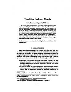
5. Numerical Examples In this section we discuss five real data examples that illustrate these models in both one- and two-dimensional situations. Example 1. High School Mathematics Test Score Data The score distribution from the mathematics section of a high-school-level basic-skills test is given in Table 1. There are 19 test items so the total numberright score, X, can take on any one of the 20 values 0, 1, 2 . . . . . 19. The sample size is N = 9889. We fit three nested loglinear models to these data, each with u = 0. Model 1 expands the two parameter model in (17) to include a cubic term; model 2 adds a fourth power-moment term to that; and model 3 adds a fifth power-moment to that. These models fit 3, 4, and 5 parameters to the data, and have the first 3, the first 4, and the first 5 sample moments as sufficient statistics, respectively. The fit statistics and degrees of freedom are given in Table 2. All three fit statistics tell a similar story. Model 3 fits well, and the difference in chi-square values between models 2 and 3 is over 10 with one degree of freedom indicating that it does a substantially better job than model 2 does. The oddities of this example are easier to see in the histogram shown in Figure 1. There is a large group of examinees concentrated at the low scores with a slow drop in frequencies over the higher scores. For many examinees this is an easy 153
Holland and Thayer
TABLE 1 Distribution of the Number-right Scores of 9889 Examinees on a 19 Item Test, Example 1 Score Frequency Score Frequency 0 153 10 536 522 308 2 470 12 456 3 568 13 518 14 628 463 5 668 15 450 6 633 16 474 7 17 564 465 18 481 8 548 19 434 9 550
TABLE 2 Chi-Square Statistic
Model 1
Model 2
Model 3
Likelihood Ratio
122.90
25.54
15.10
Pearson
118.95
25.51
15.07
Freeman-Tukey
125. I 1
25.51
15.09
15
14
Degrees of Freedom
16
test, and for a large group it is very hard. This is not the classic bell curve. The frequency for X = 13 appears to stand out from those around it. Figure 2 is a line plot of the Freeman-Tukey deviates against score value and indicates that the improvements in fit of model 3 over model 2 is not concentrated in a single place but is spread over most of the score range. The deviate for score X = 13 for model 3 is not particularly large with reference to the N(0,1) distribution, suggesting that its deviation from the rest of its neighboring score frequencies is compatible with random variation. The Normal probability plot of the Freeman-Tukey deviates given in Figure 3 also suggests that the fit of model 3 is very good. This is an example where we need a "five moment fit" to adequately reproduce the data using a Ioglinear model. Example 2. The Keats and Lord Univariate "WMi" Data
We include this example because of its historical interest. Lord (1962) and Keats (1964) used it as an example that was not fit well by a 4-parameter compound-binomial score distribution model. The W M I data come from a 30 item test scored by number right. There are 1000 examinees in the sample. Table 4 gives the score distribution for the 31 possible values, 0, I . . . . . 30. The histogram of score values in Figure 4 indicate that W M I is a relatively easy test for the examinees in the sample (i.e., it is negatively skewed), but that 154
Univariate and Bivariate Loglinear Models 0
o
Number RIItht ScOrl
FIGURE
I.
High School Mathematics Test Data Observed and Fitted Frequencies
.
/ I
2
~
•
6
6
7
ii
ii
1o
Ii
12
1~1
14
15
16
17
III
is
20
N ~ r ~ r l~lOat
FIGURE 2,
High School Mathematics Test Data Freeman-Tukey Deviates 155
Holland and Thayer 3
-
2
-
~
i
-
~
o
~
-1
=
.2
e~ 0
./. [..
I -3
-2
-1
0
I
Normal Scores FIGURE 3.
High School Mathematics
Test D a t a
o
0
I
2
3
4
5
e
7
8
9
1011121314151BITIS~92021222324252827282930
Score
FIGURE 4. 156
W.M.I. D a t a O b s e r v e d a n d F i t t e d F r e q u e n c i e s
I
I
2
3
Univariate and Bivariate Loglinear Models TABLE 3 Chi-Square Statistic
Model I
Model 2
Likelihood Ratio
41.12
25.40
Pearson
40.77
24.38
Freeman-Tukey
39.13
23.7 I
Degrees of Freedom
27
26
TABLE 4 Distribution of the Number-right Scores of 1000 Examinees on a 30 Item Test (WMI), Example 2 Score Frequency Score Frequency Score Frequency 0 0 10 5 20 37 I 0 I1 14 21 48 2 I 12 10 22 40 3 2 13 12 23 50 4 4 14 10 24 74 5 6 15 14 25 78 6 7 16 17 26 85 7 2 17 16 27 103 8 3 18 22 28 112 9 4 19 27 29 114 30 83
the score distribution has a very long left tail. We fit two nested loglinear models to these data, both with u = 0. They were, respectively, model I and model 2 of Example I, a 3- and 4-parameter model, respectively. The fit statistics and degrees of freedom are given in Table 3. Again, the message from all three goodness of fit statistics is the same. Model 2 with four parameters fits substantially better than model 1 does with three parameters. The fit of these models is illustrated in various ways in Figures 4, 5, and 6 which parallel Figures I, 2, and 3 of Example I, and indicates that model 2 is a very accurate description of the data. This example shows that the reported poor fit by the 4-parameter compoundbinomial model can be substantially improved upon by a 4-parameter loglinear score distribution model.
Example 3. A Bivariate Distribution o f Rounded Formula-Scores that Exhibit "Teeth" in One Margin This example is based on data from 26,330 examinees who took a national admissions test which included two verbal subtests. Table 5 gives the joint distribution of the observed frequencies of the rounded (to integers) formulascores (i.e., scores "corrected for guessing" in the usual way) for both of these 157
Holland and Thayer - .-,-i---. Fllelmlln-TuluFi ~ I .~ Ftleml~Ttd~/I~v~Id~alJ/ -
-
Z ~ , ~ erie
2'
Ii
po
t
•
!
n
oq,'.
/
•
i o -1
!/'?
/
Score
FIGURE 5.
W.M.I. Data Freeman-Tukey Deviates
• m D mare
"Jim
o
-3
I
-2
I
-1
Normal FIGURE 6.
158
W.M.I. Data
0
I
I
I
1
2
3
Scores
TABLE 5 Joint distribution of grouped formula scores of 26,330 examinees on two verbal tests, Example 3
~,
9 10 11 12 13 14 15 16 17 18 19 20 21 22 23 24
49.5 47.5 45.5 43.5 41.5 39.5 37.5 35.5 33.5 31.5 29.5 27.5 25.5 23.5 21.5 19.5 17.5 15.5 13.5 11.5 9.5 7.5 5.5 3.5
1
2
-7.0
-2.0
0 0 0 0 0 0 0 0 0 0 0 0 0 0 0 0 0 1 2 1 4 ! 3 4
0 0 0 0 0 0 0 0 0 0 0 0 0 l 1 2 3 7 7 8 14 12 19 24
3
4
3.0
8.0
0 0 0 0 0 0 0 0 0 0 0 2 4 9 5 26 16 27 44 48 56 45 54 51
0 0 0 0 0 0 1 1 4 4 15 17 39 41 43 87 75 111 115 102 139 82 56 44
5
6
7
8
9
13.0
18.0
23.0
28.0
33.0
0 0 0 0 0 1 0 11 20 17 47 42 71 121 101 181 141 158 213 120 122 77 59 42
0 0 0 I 2 9 16 29 63 51 126 113 186 238 178 287 205 242 187 113 104 49 38 19
0 0 2 9 11 29 41 96 148 122 217 217 329 312 230 290 194 208 149 64 49 30 19 7
0 0 7 23 30 72 83 180 263 195 361 267 390 337 234 258 131 122 101 31 35 14 14 5
I 4 17 62 65 165 158 275 420 248 395 283 333 298 147 179 104 67 45 15 9 8 2 0
10
11
12
13
14
15
16
17
18
19
38.0
43.0
48.0
53.0
58.0
63.0
68.0
73.0
78.0
83.0
36 49 53 36 17 23 5 8 2 1 1 0 0 0 0 0 0 0 0 0 0 0 0 0
34 14 23 11 8 3 1 0 0 0 0 0 0 0 0 0 0 0 0 0 0 0 0 0
I 10 28 97 118 237 196 368 379 243 329 199 232 172 113 90 35 27 20 9 I 2 0 0
5 19 74 187 129 300 243 343 312 204 246 118 132 94 42 43 23 11 6 7 2 0 0 0
13 26 i10 215 156 307 194 269 212 137 151 70 61 31 24 17 9 0 4 1 0 0 0 0
22 44 147 244 142 271 141 191 161 70 73 33 32 16 6 3 1 3 0 0 0 0 0 0
34 53 142 229 105 186 67 105 67 22 36 9 12 5 4 2 I 0 0 0 0 0 0 0
49 52 141 154 85 109 64 57 20 9 18 4 3 0 0 0 0 0 0 0 0 0 0 0
36 43 106 97 41 34 24 21 12 3 5 1 0 0 0 0 0 0 0 0 0 0 0 0
7 4 6 4 0 1 0 "0 0 0 0 0 0 0 0 0 0 0 0 0 0 0 0 0
"" c~
TABLE 5---Continued
Joint distribution of grouped formula scores of 26,330 examinees on two verbal tests, Example 3
25 26 27 28 29
1.5 -0.5 -2.5 -4.5 -6.5
1
2
-7.0
-2.0
2 3 0 0 0
6 13 3 1 1
3
4
3.0
8.0
18 18 5 6 2
22 13 8 3 0
5
6
7
8
9
13.0
18.0
23.0
28.0
4 6 0 0 0
2 0 0 0 0
0 0 0 0 0
!1 8 4 I 0
10
11
12
13
14
15
16
17
18
19
33.0
38.0
43.0
48.0
53.0
58.0
63.0
68.0
73.0
78.0
83.0
0 0 0 0 0
0 0 0 0 0
0 0 0 0 0
0 0 0 0 0
0 0 0 0 0
0 0 0 0 0
0 0 0 0 0
0 0 0 0 0
0 0 0 0 0
0 0 0 0 0
0 0 0 0 0
Univariate and Bivariate Loglinear Models
verbal subtests. The scores for the row test, X, are grouped into 29 intervals, whereas those of the column test, Y, are grouped into 19 intervals. We have used the midpoints of the intervals as the "scores" for each interval. For the rows the midpoints range from 49.5 to - 6.5 in steps of 2, and for the columns they range from - 7 to 83 in steps of 5. Figures 7 and 8 show the row and column frequencies (along with the fitted values from several models). It is evident that the row distribution exhibits "teeth" in the sense that there is a regular pattern of cells wherein the frequencies are much lower than those of the neighboring cells. This phenomenon is due to the use of rounded formula scores and the concomitant presence of substantial amounts of omitting on the row test items. The distribution of the column test does not exhibit teeth because of the more severe grouping that has been done in constructing Table 5 - - f i v e scores in a column-interval versus two in a rowinterval. An examination of Table 5 shows that the teeth in the marginal distribution, X, propagate themselves into frequencies of the body of the table. This phenomenon has nothing to do with sampling variability, and we will need to account for it in the models we use for these data. Our approach to finding a good model for the joint distribution is to first find adequate models for the margins of the joint distribution (i.e., the "outside") and then to use these to find a good model for the entire joint distribution (i.e., the "inside"). We do this because important features of the marginal distributions constrain the joint distribution, and it is easier to look at one variable at a time. In order to fit the two smooth trends in the row frequencies seen in Figure 7, we divided the rows into those with row numbers given by S = 12, 5, 7, 10, 12, 15, 17, 20, 22, 25, 27 } and the rest. The rows indexed by S have frequencies that are lower than their neighbors due to rounded formula s c o r e s - - t o ascertain this we did not use the frequencies themselves, but other information about the test. In this case it is the large number of test t a k e r s w h o omitted no items so that S is determined by the scores that are impossible to achieve by the rounded formula scores of such test takers. Expanding the models illustrated in (21) and (22), we constructed a model for the row distribution that has as its sufficient statistics: the first five moments of the row distribution, plus the total of the cell frequencies in the rows indexed by S, plus the first five moments of the row distribution restricted to the cells in S. This has the effect of "fitting the teeth" as we see from the fitted values in Figure 7. We also constructed a model for the column distribution that has its first five moments as its sufficient statistics because there was no need to fit "teeth" to the column distribution. Finally, to get a joint distribution for X and Y, we let them be independent with these special models for their marginal distributions so that there were no terms in the model for the joint distribution involving products of X and Y values. We called this initial model, model 1. It has 5+5+1+5 = 16 parameters out of a possible 29x19 - 1 = 550. The fitted marginal distributions for X and Y from model 1 are shown in Figures 7 and 8, respectively. The likelihood-ratio chiTsquare statistic for model I is 24,187.26 on 161
Holland and Thayer
,11111
aeo ,
o
•4 n
4.s .21 -oJ
t.s
1.5 i . ~
ll
7 . s t s I I . s 11.5 I I S ST.~I I t . s I I.S 13.5 ~5 5 l T . J l ' l S I I.J ' l l 5 '15,S 37.~ 19.5 ~I.S 41.5 I S S i ~ . l *O.S
Rounded Formczls S c w t s
FIGURE 7. Rounded Formula Scores Row Margins: Observed and Fitted Frequencies
~"]
o
Q,,~.,,
/
~
~mKL~
-t
"
I
. . . .
o
•7
,2
S
e
lS
lS
2~
2a
SS
Se
4#
Rounded Formula
FIGURE 8. Roututed Formula Scores Column Margins. Observed and Fitted Frequencies 162
.8
5S
nl
eS
e8
73
7a
e3
Univariate and Bivariate Loglinear Models
550-16 = 534 degrees of freedom indicating the obvious need to include parameters in the model for the association between X and Y. While Figures 7 and 8 show that model I reproduces the general shape of the marginal distributions, when we look more closely in Figures 9 through 12 at these fitted distributions using the Freeman-Tukey residuals to compare the observed and fitted marginal distributions of X and Y we see that there are a few discrepancies that are not just sampling error. Because this is mostly due to the huge sample size in this example, and because the discrepancies show no systematic pattern, we will not attempt to improve on the fit of the marginal distributions in this example. To address the association between X and Y, we first added a single parameter to model 1 to get model 2, the parameter associated with a term corresponding to the cross product in (24). This adds the correlation between X and Y to the previous list of sufficient statistics. This has a substantial effect on improving the model fit--the likelihood-ratio chi-square statistic for model 2 is 577.72 on 533 degrees of freedom indicating a remarkably good fit considering the large amount of data in the sample. In order to check the adequacy of this fit, we created model 3 that added to model 2 the three power cross-moments of the form X2y, XY 2, and X2y 2. Model 3 then has 20 parameters and a likelihoodratio chi-square statistic of 435.48 on 530 degrees of freedom. The difference in the likelihood-ratio chi-squares for models 2 and 3 is 142.24 with 3 degrees of
•
FTIO~iO~L~I $
Ar ~..~ .,%
" ,[B
. 6.B
.
. I.s
. la,a
. 17 8
, ll.s
.
. 25.~
.
. zo.s
. a:.s
. :T.S
. 41.s
.
, 4s.5
.
, 4|.B
Roandld Formuls Seoru
FIGURE 9. Rounded Formula Scores Row Margins: Freeman-Tukey Deviates 163
Holland and Thayer
l i /
~ . 7
.
-3
.
.
3
.
.
.
"
e
lS
10
'
=3
"
'
"
3e
slt
"
"
"
3e
45
"
'
"
4a
'
ss
"
.
.
ee
.
es
.
.
ee
"
TS
Rmmdl~l Fm'm~ta Seer~
10. Rounded Formula Scores Column Margins." Freeman-Tukey Deviates FIGURE
y il
e~
-1
E r~
-2
-3
"[
I
I
-2
-I
0
Normal FIGURE
11.
Row Margins 164
Rounded Formula Scores
I
I
Scores
t 2
7e
'
e3
Univariate and Bivariate Loglinear Models
0
ca
r.~
I -3
-2
I -I
I 0
I I
I 2
:
Normal Scores FIGURE 12.
Rounded Formula Scores Column Margins
freedom, a sizable reduction that suggests that model 2 can be improved by the addition of the extra association parameters in model 3. Figure 13 is a Normal probability plot of the Freeman-Tukey residuals for all of the cells in Table 5 using the fitted values from model 3. While there are some problems in using these residuals when there are so many zero frequencies, the plot indicates that the few large Freeman-Tukey residuals are not larger than one would expect from the examination of so many approximate Normal deviates. In the bivariate case, we believe that plots like those in Figures 14 through 19 give more incisive assessments of the improvement in the fit that model 3 has over model 2 than do the measures of overall fit like the Chi-square statistics or the detailed cell-by-cell assessment by the Freeman-Tukey residuals. The first three plots, Figures 14 to 16, concern the conditional distribution of the column scores given the row scores, while the last three, Figures 17 to 19, concern the conditional distribution of the row scores given the column scores. Each plot shows information for both model 2 (dashed lines connecting hollow boxes) and model 3 (solid lines connecting solid diamonds). The vertical axes in all plots are Z-values for the quantities defined in (55), (56) and (57). The horizontal axes are the values of the conditioning variable, column or row as the case may be. These plots give us a detailed summary of how well the model fits the first three moments of each of the conditional distributions: Row (X) given Y = Yi, and Column (Y) given X = x i. 165
Holland and Thayer 3
2
~o ~,,-I
-3
I -3
-2
-1
0
Normal
FIGURE 13.
1
2
3
Scores
Rounded Formula Scores
1
.,./i /:' ~v v 1
.i/ f ~-IB S
-2'.5
1.6
5.5
9.6
13.6
l?.l
21.5
25,8
21.5
33.5
Roanded Formu~ Scor~ (Rows)
FIGURE 14. Rounded Formula Scores Z Values f o r Mean Column Scores Conditional on Row Scores
166
37.5
41.§
4B.§
4g.S
Univariate and Bivariate Loglinear Models
ZSmL~
\
•
-6.S
-i.s
;.S
S.5
O.S
I:.S
.
I?,s
,
.
RI.s
,
.
28.s
.
.
211.|
R o u m l ~ Formula, S t e m
. 3|.fl
.
.
.
37,6
, 41.5
48,8
40.8
(]~om)
FIGURE 15. Rounded Formula Scores Z Values for Standard Deviation of Column Scores Conditional on Row Scores
i..'I ...,,,
"2"
J J
•e.s
,
.:.s
r
.
1.5
.
.
.
.
s.s
'
e.~
l:.s
'
I?,s
J
J
1
EI.S
II~nded Formnla ~
'
tS.S
r
'
2:.S
J
"
8S.6
:7.S
J
'
41.S
J
4S.5
1
'
4LI
(Eo~)
FIGURE 16. Rounded Formula Scores Z Values for Skewness of Column Scores Conditional or, Row Scores 167
Holland and Thayer
/!
/~
tAJ i
/S//'j
V ~v i
j.
- -
~
z um~3 z m LJn*
IIo~ad~l Formula Scercs (Columltl)
FIGURE 17. Rounded Formula Scores Z Valuesfor Mean Row Scores Conditional on Column Scores
/
',,
.i; '.,.'
.
6
IL~n4~d Ire*l,din ~
(CMmams)
FIGURE 18. Rounded Formula Scores Z Valuesfor Standard Deviation of Row Scores Conditional on Column Scores 168
Univariate and Bivariate Loglinear Models ---,o---. ~ - -
/",,, /
ZJI~t.lnl
",,,
.
o
IJcml|
A
A
;
\
] './ ,g •7
.I
3
a
13
II
I$
lID
31
38
43
"/
41
/"
/
53
~l
6~J
66
71
78
81
Rounded Formuls Scores (Columns)
FIGURE 19. Rounded Formula Scores Z Valuesfor Skewness of Rwo Scores Conditional on Column Scores
Figure 14 shows that while there are systematic and statistically significant deviations of the row means of the fitted distribution from those of the data for model 2, those for model 3 are more satisfactory, i.e., the Z-values are more like random N(0,1) noise. The same is true for the row variances in Figure 15, though the fits are more similar than in Figure 14. The Z-values for the row skewnesses are in Figure 16 and indicate a similar improvement of model 3 over model 2. Figures 17-19 show the improvement in the fit of model 3 over that of model 2 even more dramatically. Several of the Z-values for the column moments exceed 3.0 in magnitude for all three moments. In summary, model 3 represents the row and column conditional distributions of the data very well. This would give us confidence in using the smoothed distribution for a variety of uses. In particular, this example comes from data used for test equating where the row correspond to the values of an anchor test and the columns to the values of one of the tests to be equated. In such applications the conditional distributions play important roles. Example 4. The Bivariate Milk-Yield Data
Kendall and Stewart (1963, p. 29) include data on 4912 cows classified by age in years and yield (in gallons) of milk per week reported in Tocher (1928). While not an educational example, these data show some interesting features 169
Holland and Thayer TABLE 6
Joint Distribution of Milk Yield per Week (rows) by Age in Years (columns) for 4,912 Ayrshire Cows, Example 4
5 6
7 8 9
10 11 12
13 14 15 16
17 18 19 20 21 22 23 24 25 26
27
Row and Col Vats 8 9 10 11 12 13 14 15 16 17 18 19 20 21 22 23 24 25 26 27 28 29 30 31 32 33 34
1
2
3
4
5
6
7
8
9
10
11
12
13
14
15
16
3
4
5
6
7
8
9
10
II
12
13
14
15
16
17
18
0 0 3 2 2 9 I1 I1 15 16 11 10 8 3 5 1 2 3 0 0 0 0 0 0 0 0 0
0 2 5 10 25 76 76 115 149 148 146 117 97 63 42 19 20 10 7 2 0 0 0 0 0 0 0
0 2 1 8 17 29 57 79 !19 131 132 112 107 93 63 33 23 15 13 7 2 2 0 2 0 0 0
0 0 I 7 9 18 38 43 74 94 83 113 79 88 49 38 34 22 7 9 I 2 0 1 2 0 0
0 1 3 1 5 9 23 34 59 58 73 87 69 70 45 38 27 17 4 5 4 4 0 0 0 0 0
0 0 0 0 4 2 9 24 23 34 49 51 51 49 32 27 19 20 15 5 2 1 2 0 0 0 0
0 0 0 I 4 4 7 II 23 32 39 35 25 31 14 17 13 8 2 4 I 3 0 2 0 0 0
0 0 0 0 2 I 6 8 16 15 22 33 30 29 18 17 9 10 4 2 I 0 0 0 0 0 0
1 0 0 2 I 1 4 4 9 12 17 11 13 9 10 12 3 3 2 0 2 3 2 0 0 0 1
0 0 0 1 I I 2 5 7 6 6 10 10 7 3 7 2 4 3 0 0 0 0 0 0 0 0
0 0 0 2 0 0 3 1 4 5 5 2 3 4 I 1 1 0 1 0 0 0 0 0 0 I 0
0 0 0 1 0 I 0 2 0 0 I 3 3 0 2 2 0 0 0 0 0 0 0 0 0 0 0
0 0 0 0 0 0 0 I 0 1 I 1 0 1 0 2 0 0 0 0 0 0 0 0 0 0 0
0 0 0 0 I 0 0 0 0 0 0 0 0 0 0 0 0 0 0 1 0 0 0 0 0 0 0
0 0 0 0 0 0 0 I I 0 0 0 1 1 0 0 0 0 0 0 0 0 0 0 0 0 0
0 0 0 0 0 0 0 0 0 0 0 I 0 0 0 0 0 0 0 0 0 0 0 0 0 0 0
that occur in other applications. The frequencies for this bivariate distribution are displayed in Table 6. The values for milk yield range from 8 to 34 gallons per week, and the ages range from 3 to 18 years. Figures 20 and 21 show the row and c o l u m n frequencies (along with the fitted values from two models). The row distribution (milk yield) shows a simple unimodal shape, while the c o l u m n distribution is very positively skewed and the frequency for age 3 is considerably smaller than those o f its neighboring ages. After s o m e initial exploration, we decided to fit the frequency for age 3 exactly and smooth the other frequencies. This can be done fairly well with a loglinear m o d e l that has the mean, variance and skewnesses as the sufficient statistics for 170
Univariate and Bivariate Loglinear Models
4C0
.-
=oo
ioo
o 9
10 I 1 12 13 ~4 15 18 17 18 1D 20 21 22 2S 24 i S 26 27 88 21 SO S l ~2 S~ 34
Yield of ~
per ~
(J~Ums)
FIGURE 20. Milk Yield Data Row Margins." Observed and Fitted Frequencies
4
n
n
I
I0
1~
II
I]
14
In
16
i?
i]
In YrLrs
Milk Yield Data Column Margins: Observed and Fitted Frequencies
FIGURE 21.
171
Holland and Thayer
the row (milk yield) distribution, but for the column (age) distribution has the mean, variance and the frequency of age 3 as the sufficient statistics. To complete the model, we considered two cases for the association between milk yield and age. In model 1 we included the product term, XY, so that the added sufficient statistic is the sample correlation or covariance. In model 2, we added the additional product terms, X2Y, XY z, and X2Y z, as we did for model 3 of Example 3. Figures 20 and 21 show the observed and fitted marginal distributions for these two models. More detailed comparisons are given by the Freeman-Tukey residuals in Figures 22 and 23. These plots suggest that the fit of the row marginal is satisfactory, but that it might be possible to improve on the fit of the column distribution. We will not pursue this improvement here because the fitted distribution is satisfactory for our minimal needs, and the Normal probability plots of the Freeman-Tukey residuals for the fits of both marginal do not seem to indicate any particularly large discrepancies. This example shows that models that vary only the "association" parameters can have effects on the marginal distributions as well. The row distribution is virtually the same for the two models, but there are noticeable differences between them in the column distribution. The usual chi-square fit statistics for models 1 and 2 are shown in Table 7. In this example we see that the fit statistics do not necessarily agree. The pattern
•
• -
-
F'r~
MoUld 1
FI'Oo~ Jd~el 2 ZIm
A ,m L/
÷ o
.1.
|
10
11 12
13
14
13
18
17 18
19 20 21
22
23 24 =8 =6
Ylr.]d o f m i l k per week ( p l l o m )
FIGURE 22. Milk Yield Row Margins." Freeman-Tukey Deviates 172
27
28 2D 30 31
32 31
34
Univariate and Bivariate Loglinear Models
2
1
h w
J
"2
;
~
~
;
~
~
;o Age la
fi
,'2
,'s
,',
;6
,'e
,;
,'e
years
Milk Yield Column Margins: Freeman-Tukey Deviates FIGURE 23.
2 e,t
0
0 dll el
d~
-2
/ I -2
I -I
I 0
Normal
FIGURE 24.
I I
I 2
Scores
Milk Yield Data
Row Margins 173
Holland and Thayer
/ e,I
2
o
rX
i
o
el
.~
-2
I
-3
-3
-2
-I
0
I
Normal
2
Scores
FIGURE 25. Milk Yield Data Column Margins
TABLE 7 Chi-Square Statistic
Model 1
Model 2
Likelihood Ratio
451.71
347.00
I 012.23
650.12
Pearson Freeman-Tukey
357.69
267.84
Degrees of Freedom
424
421
where the Pearson Chi-square statistic is substantially larger than the other two often happens and is usually due to a large number of small cell frequencies in the data. It is evident that while both models fit fairly well, the improvement of model 2 over model I is significant--the difference in likelihood-ratio chisquares is 104.71 on 3 degrees of freedom. The Normal probability plot of the Freeman-Tukey residuals for all of the cells for model 2 is displayed in Figure 26. It indicates that the largest residuals are no larger than one would expect to find in examining so many o f them. Again, we can use the Z-values for the row and column fitted conditional distributions to see in more detail how the models compare. Figures 27-32 give these Z-values in the same order as Figures 14-19 did for Example 3. 174
Univariate and Bivariate Loglinear Models 3
-2
• • i~
-3
-3
-2
-I
0
2
3
Normal Scorn
F I G U R E 26.
Milk Yield Data ',
:
- -
zmune
8 .N
\
\ / / 8
7
8
9
10
It
l|
/
13
A l e In Y e l r l
F I G U R E 27. Milk Yield Data Z Values for Mean Yield of Milk in Gallons Conditional on Age in Years 175
Holland and Thayer
-
-
zem LrQ
Ale In ¥ ~ n
FIGURE 28. Milk Yield Data Z Values for Standard Deviations of Yield of Milk in Gallons Conditional on Age in Years
..... ~
",.
! i
•
4
6
II
7
|
|
10
11
12
13
14
16
111
17
III
AI* In ¥ ~ t ~
FIGURE 29. Milk Yield Data Z Values for Skewness of Yield of Milk in Gallons Conditional on Age in Years
176
Univariate and Bivariate Loglinear Models
J
Z~sawlll
r /
/i
. . . . B I O 11 1 2
i . 1 3 14
. . . . . 1 6 10 I ? 18
. II
. . . . . . . . . . 2 0 21 2R Ea 1 4 a 8 Rq} ~?
. . . ~e a l l ~lO I $
31 S3 3 4
Y i e l d o f Unllk Ira" w e e k (IzJ~m)
FIGURE 30. Milk Yield Data Z Values for Mean Age in Years Conditional on Yield of Milk Per Week in Gallons
/-
- -
ZmCI~
\
i
..,,
I
/ I
10
II
I~
IS
14
ID
II
17 I 1
11 I 0
Jl
II
Yltld d m l ~ P e r ~
2 1 1 4 Z~ I n
27 II
IJ
~ 0 ~1
~
~
~4
(pUom)
FIGURE 31.
Milk yield Data Z Valuesfor Standard Deviation of Age in Years Conditional on Yield of Milk Per Week in Gallons 177
Holland and Thayer
/
9
10 11 12 13 14 16 111 17 18 19 I 0
II
12 ;~3 24 25 16 ] 7
IfO 2D 30 31 32 33 34
Y l d d of m i ~ p e r w ~ k (pfloQs)
FIGURE 32. Milk Yield Data Z Valuesfor Skewness of Age in Years Conditional on Yield of Milk Per Week in Gallons
Figure 27 shows a noticeable improvement in the fitted yield means for each age for model 2 over model I, but the fitted variances and skewnesses of the yield distributions for each age are about the same for the two models as seen in Figures 28 and 29. Figures 30-32 are for the age distributions for each yield level, and each shows a big improvement of model 2 over model 1. However, most of our interest in these data goes one way, i.e., from age to yield. Figure 33 shows the observed mean yields for each age and the corresponding fitted mean yields for the two models. Both do poorly in different ways for the highest ages where there is little data, but the improvement of model 2 over model 1 in the cases where the data are plentiful is very clear from this display and verifies the residual plot in Figure 28.
Example 5. A Square Triangular Table of Scores That Can Only Improve
Bishop et al. (1975, page 197) include data on 121 stroke patients who were given physical disability ratings on admission (X) and on discharge (Y) from a hospital. Because no patient was discharged if he or she had become worse, a patient's score on discharge could never be lower than it was on admission, i.e., X --< Y. This results in the triangular array displayed in Table 8. In the original data, the ratings were the ordered categories A to E. We have replaced these with 178
Univariate and Bivariate Loglinear Models • .... ~ - - .
UmlCl~wv~lvl*~ I,,11m,km,a a ~ l ~4"" ¢
. J " Y
=1
.,...,"
.
Io
le
t7
X 16
IS.
14-
4
5
8
?
(I
9
10
I1
12
IS
~4
~5
16
1?
18
.4p In Ym"J
FIGURE 33.
Regression of Milk )7eld on Age in Years
the integer values I = E, 2 = D . . . . , A = 5, so that higher scores indicate less disability. These data have been used to illustrate tests of the quasi-independence model, which correspond in this case to models where there are no association parameters. It should be pointed out that the usual model of quasi-independence in this setting fits the row and column distributions exactly and has no further association beyond that which is forced by the triangular nature of the data (Holland & Wang, 1987). In our case, this can be achieved by fitting a model with the first four power moments for the rows and the same four corresponding power moments for the columns because a distribution with only five possible values is completely determined by its first four moments. Table 9 gives the fitted values found in this way. They agree with the values given in Bishop et al. (1975) for the usual model of quasi-independence except for rounding. The likelihood ratio chi-square value for this model is 9.60 with ! 5-1-8 = 6 degrees of freedom, with an associated p-value of 0.14 indicating an acceptable fit. The only FreemanTukey deviate of any size ( - 1.95) is the one for the (2,2) cell where the observed frequency is 1 and the fitted cell value is 4.52. The interpretation is that while patients did get better--the mean score is 2.34 on admission and is 4.18 on discharge--there is no relation between their status at admission and at discharge except that which is forced by the constraint that they are not discharged unless they improve, i.e., unless X --< Y. 179
Holland and Thayer
TABLE 8 Distribution of Disability Scores for 121 Stroke Patients on Admission (rows) and on Discharge (columns), Example 5. Scores
1
1
8
2 3 4 5 Total
0 0 0 0
2 15 1 0 0 0 16
3 12 4 4 0 0 20
4 23 I0 4 5 0 42
5 11 9 6 4 5 35
Total 69 24 14 9 5 121
TABLE 9 Fitted values for the data in Table 8fitting the first four power moments to the row and column distributions and no association parameters (i.e., quasi-independence) Scores I 2 3
I 8.00 0 0
2 11.48 4.52 0
3 11.93 4.69 3.37
4 21.92 8.63 6.20 5.25
Total
8.00
16.00
19.99
42.0
5 15.66 6.16 4.43 3.75 5.00 35.00
Total 68.99 24.00 14.00 9.00 5.00 120.99
Our interest in this example is to see if any insight into the data accrues if we fit fewer moments of the row and column distributions and then fit a single association parameter to test for quasi-independence. This has the potential of producing a more powerful test than the overall likelihood ratio chi-square test that has 6 degrees of freedom that was reported above. To this end we fit two additional models. Model 1 is just like the quasi-independence model except that only two moments are fit to the row and the column marginal distributions. Model 2 has this same feature and in addition fits a single association parameter that corresponds to the correlation between X and Y. Both models may be represented by the Ioglinear model in (24) subject to the added restriction that x i