(ALIS), is proposed to compute small failure probabilities encountered in high- .... The estimate Ëpis in (7) has the same statistical properties as Ëpmc in (3), i.e., .... an estimate of Zαj+1 /Zαj since it converges to 1/4 when n â â rather than 1/2.
ESTIMATION OF SMALL FAILURE PROBABILITIES IN HIGH DIMENSIONS BY ADAPTIVE LINKED IMPORTANCE SAMPLING L.S. Katafygiotis1 and K.M. Zuev1 1
Hong Kong University of Science and Technology, Department of Civil Engineering, Clear Water Bay, Kowloon, Hong Kong, China, email: {lambros, zuev}@ust.hk
Key words: Reliability, Importance sampling, Subset simulation, Bridging, MCMC. Abstaract. A novel simulation approach, called Adaptive Linked Importance Sampling (ALIS), is proposed to compute small failure probabilities encountered in high-dimensional reliability analysis of engineering systems. It was shown by Au and Beck (2003) that Importance Sampling (IS) does generally not work in high dimensions. A geometric understanding of why this is true when one uses a fixed importance sampling density (ISD) was given in Katafygiotis and Zuev (2006). In this paper we introduce an algorithm referred to as Adaptive Linked Importance Sampling (ALIS). The basic idea of ALIS is instead of using a fixed ISD, as done in standard IS, to use a family of intermediate distributions that will converge to the target optimal ISD corresponding to the conditional probability given the failure event. We show that Subset Simulation (SS), which was introduced by Au and Beck (2001), does correspond to a special case of ALIS where the intermediate ISD’s are chosen to correspond to the conditional distributions given adaptively chosen intermediate nested failure events. However, the general formulation of ALIS allows for a much richer choice of intermediate ISD’s. As the concept of subsets is not a central feature of ALIS, the failure probability is not any longer expressed as a product of conditional failure probabilities as in the case of subset simulation. Starting with a one-dimensional example we demonstrate that ALIS can offer drastic improvements over subset simulation. In particular, we show that the choice of intermediate ISD’s prescribed by subset simulation is far from optimal. The generalization to high-dimensions is discussed. The accuracy and efficiency of the method is demonstrated with numerical examples.
1
1 INTRODUCTION In reliability engineering our task is to calculate the reliability or equivalently the probability of failure of a system under given loading conditions. The mathematical models of the input load x and the system output f (x) are random vectors x ∈ RN with joint probability density function (PDF) π0 and function f : RN → R+ correspondingly. For example, if our system corresponds to a tall building, the input may represent wind velocities along the building height and the output may represent the maximum roof displacement or the maximum interstory drift (absolute value) under the given wind load. Define the failure domain F as the set of inputs that lead to the exceedance of some prescribed critical threshold b ∈ R+ : F = {x ∈ RN |f (x) > b} (1) We are interested in the probability of failure : Z Z IF (x)π0 (x)dx = Eπ0 [IF ] pF = P (x ∈ F ) = π0 (x)dx = F
(2)
RN
where IF is the indicator function (= 1 if x ∈ F , = 0 otherwise) and Eπ0 denotes expectation with respect to the distribution π0 , where π0 denotes the PDF of the input random variables x. Among all procedures developed for estimation of pF , a prominent position is held by stochastic simulation methods. The expression of pF as a mathematical expectation (2) renders standard Monte Carlo method [8] directly applicable, where pF is estimated as a sample average of IF over independent and identically distributed samples of x drawn from the PDF π0 : n 1X IF (x(k) ), x(k) ∼ π0 (3) pˆmc = n k=1 This estimate is unbiased and the coefficient of variation (COV), serving as a measure of the statistical error, is s (1 − pF ) δmc = (4) npF Although standard Monte Carlo is independent of the dimension N of the parameter space, it is inefficient in estimating small probabilities because it requires a large number of samples (∼ 1/pF ) to achieve an acceptable level of accuracy. For example, if pF = 10−4 and we want to achieve an accuracy of δmc = 10% we need approximately 106 samples. Therefore, standard Monte Carlo becomes computationally prohibitive for our problems of interest involving small failure probabilities. Importance Sampling is a fundamental technique in stochastic simulation that tries to reduce the COV of the Monte Carlo estimate. In statistical physics literature this procedure is also called “simple importance sampling” and “free energy perturbation”. The basic idea of Importance Sampling is to generate more samples in the important region of the failure domain, i.e., in the region of the failure domain that contains most of the probability mass and, therefore, contributes mostly to the integral (2). Roughly speaking standard Monte Carlo does not work because the vast majority of terms in the sum (3) are zero and only very few are equal to one. Using Importance Sampling we 2
want instead of estimating pF as the average of a vast majority of 0’s and, occasionally some (if any) 1’s, to calculate it as the average of less zeros and many more nonzero small numbers, each being ideally of the order of pF . Specifically, let π1 be any PDF on the parameter space RN such that its support (domain where π1 is not zero) contains the intersection of failure domain with the support of π0 : supp π1 ⊃ F ∩ supp π0 (5) Then we can rewrite the probability integral (2) as follows : · ¸ Z Z π0 (x) π0 pF = IF (x)π0 (x)dx = IF (x) π1 (x)dx = Eπ1 IF π1 (x) π1 RN
(6)
RN
Suppose that we are able to generate random samples from π1 , called importance sampling density (ISD), and compute the value of π1 (x) easily for any given x. Then similarly to (3) we have : n 1X π0 (x(k) ) pˆis = , x(k) ∼ π1 (7) IF (x(k) ) n k=1 π1 (x(k) ) Note that the standard Monte Carlo method is a special case of Importance Sampling when π1 = π0 . The estimate pˆis in (7) has the same statistical properties as pˆmc in (3), i.e., it is unbiased and it converges to pF with probability 1. Choosing π1 in some appropriate way we hope to be able to reduce the COV. It was shown by Au and Beck [2] that Importance Sampling does generally not work in high dimensions. A geometric understanding of why this is true was given by Katafygiotis and Zuev in [5]. In that paper it is shown that Importance Sampling is inapplicable in high dimensions because it is practically impossible to select a fixed ISD such that the samples generated by it cover the important region of the failure domain given the fact that the geometry of this important region is generally very complex and unknown a priori. In this paper we introduce an algorithm called Adaptive Linked Importance Sampling (ALIS) that is based on the methodology developed in [9]. We start from the description of all constructions that are needed. 2 PROPOSED METHODOLOGY We proceed from the classical Importance Sampling that was described above. It is easy to see that the theoretically optimal choice of π1 is the conditional PDF : π1opt (x) = π0 (x|F ) =
π0 (x)IF (x) pF
(8)
For this ISD the estimate (7) is pis = pF for any number of samples n (even for n = 1) with resulting COV δis = 0. We can conclude that the problem of estimating the failure probability is equivalent to estimating the normalizing constant for the following “optimal” non-normalized density function : popt 1 (x) = π0 (x)IF (x)
(9)
Now we will reformulate the problem of estimating the failure probability in that of estimating the ratio of the normalizing constants of two distributions. 3
2.1 Reformulation of the problem Consider two PDFs π0 and π1 on the same space RN : π0 (x) =
p0 (x) , Z0
π1 (x) =
p1 (x) Z1
(10)
where Z0 and Z1 are the corresponding normalizing constants ensuring the total probability is equal to one. Suppose that we are not able to directly compute π0 and π1 since we do not know the normalizing constants Z0 and Z1 , but p0 and p1 are known pointwise. Our goal is to find a Monte Carlo estimate for the ratio r=
Z1 Z0
(11)
Assuming this problem can be tackled, the estimation of failure probability easily follows by appropriately choosing p0 and p1 : p0 (x) = π0 (x) Z0 = 1 p1 (x) = π0 (x)IF (x) Z1 = pF
⇒ r = pF
(12)
This observation links the problem of estimating failure probabilities to two other extensively researched problems that can also be considered as problems of estimating the ratio of normalizing constants : • Finding the free energy of a physical system (Statistical Physics), • Finding the marginal likelihood of a Bayesian statistical model (Bayesian Statistics) In this paper we will address the problem of reliability estimation as a special case of calculating the ratio r of normalizing constants of two distributions. Using (10), (11) it is follows that · ¸ Z Z p1 Z1 Z1 p1 (x) Eπ0 = π0 (x)dx = π1 (x)dx = (13) p0 p0 (x) Z0 Z0 RN
RN
This means that we can estimate r by n
rˆmc(sis) =
1 X p1 (x(k) ) , n k=1 p0 (x(k) )
x(k) ∼ π0
(14)
In the context of failure probabilities, i.e., using (12), one can easily recognize that (14) becomes exactly the expression for estimating pF using standard Monte Carlo. In statistical physics literature (14) is also known as the Simple Importance Sampling (SIS) estimate. Now we turn to the idea of intermediate distributions. 2.2 Introduction of intermediate distributions If π0 and π1 are not close enough, the estimate (14) will be improper: the variance of this estimate will be very large. In such a situation, it may be possible to obtain a good estimate by introducing artificial intermediate distributions (AID’s). 4
Let us define a sequence pα0 , . . . , pαm of non-normalized (or unnormalized) density functions (UDF) using 0 = α0 < α1 < . . . < αm−1 < αm = 1, so that the first and last functions in the sequence are p0 and p1 with the intermediate UDF’s interpolating R between them. Let Zα = pα (x)dx and πα0 , . . . , παm denote the corresponding sequence of normalizing constants and PDFs, respectively. Then we can represent the ratio r = Z1 /Z0 as follows : Zα Z1 Zα1 Zα2 Z1 = . . . m−1 (15) Z0 Z0 Zα1 Zαm−2 Zαm−1 Now, if παj and παj+1 are sufficiently close and we can sample from παj , we can accurately estimate each factor Zαj+1 /Zαj using simple importance sampling (14), and from these estimates obtain an estimate for r : Ã n ! (k) m−1 Y 1X pαj+1 (xj ) (k) rˆgis = (16) , x j ∼ π αj (k) n p (x ) α j j=0 j k=1 We will refer to (16) as Generalized Importance Sampling (GIS). A novel procedure for evaluating failure probabilities called Subset Simulation was suggested by Au and Beck in [1]. The main idea of this method is as follows. Given a failure domain F let RN = Fα0 ⊃ Fα1 ⊃ . . . ⊃ Fαm = F be a filtration, in other words a sequence of failure events such that Fαk = ∩kj=0 Fαj . In terms of the representation (1), the failure events Fαj can be chosen as follows : Fαj = {x ∈ RN |f (x) > αj b} (17) Using the definition of conditional probability it can be shown that pF =
m−1 Y
P (Fαj+1 |Fαj )
(18)
j=0
The main observation is that, even if pF is small, by choosing m and Fαj , j = 1, . . . , m − 1 appropriately, the conditional probabilities can be made large enough for efficient evaluation using simulations. Each factor in (18) is approximated by n
1X IF (x(k) ), Pb(Fαj+1 |Fαj ) = n k=1 αj+1
x(k) ∼ π0 (·|Fαj )
(19)
It follows that Subset Simulation is exactly Generalized Importance Sampling with specific intermediate distributions : παj (x) = π0 (x|Fαj ),
j = 0, . . . , m
(20)
Intuition suggest that it is rather unlikely for the family of conditional intermediate distributions (20) with sharp boundaries to be optimal for estimating failure probability. Indeed, our numerical examples will show that this family of AID’s is far from optimal and, therefore, there is room to further improve efficiency beyond that offered by Subset Simulation. Here we propose two smooth families of AIDs designed for reliability problems. First, returning to the definition of the failure domain (1), define the limit state function : Φ(x) = b − f (x), 5
(21)
so that failure domain F is defined as the subset of RN where Φ is negative. Now we are define the following two families of non-normalized AIDs: pIα (x) = π0 (x) min{e−αΦ(x) , 1}
(22)
π0 (x) 1 + eαΦ(x) It is easy to check, that for both distributions we have: pII α (x) =
(23)
lim pα (x) = p0 (x)IF (x) = p∞ (x)
(24)
α→+∞
Although before it was assumed that α ∈ [0, 1], in (22), (23) the α belongs in the ray α ∈ [0, +∞]. Obviously this is not of fundamental importance. We will refer to (22), (23) as to the distributions of the first and the second types correspondingly. Note, that for the first type distributions p0 = π0 and Z0 = 1 as in (12), but for the second ones we have p0 = π0 /2 and therefore Z0 = 0.5. Again this can be easily incorporated in the expression for the estimate of pF . Specifically, as can be easily derived from (11) and (12), one simply has to multiply the estimate for r by Z0 , i.e., pF = 0.5r. 2.3 Bridging There is a potential problem one needs to be aware of when using intermediate distributions and that is the following. If the distributions {πα } are not nested, one can not hope to estimate Zαj+1 /Zαj by sampling just from παj . Indeed, this can be easily demonstrated with the following example involving uniform distributions. Let pαj = I[0,4] and pαj+1 = I[3,5] , so that Zαj = 4, Zαj+1 = 2 and Zαj+1 /Zαj = 1/2. Suppose we have n points drawn uniformly from [0, 4], i.e. from παj . The fraction of these that lie in [3, 5], i.e. the simple importance sampling estimate (14), will obviously not give an estimate of Zαj+1 /Zαj since it converges to 1/4 when n → ∞ rather than 1/2. Instead it will be an estimate of Z∗ /Zαj , where Z∗ is the length of [3, 4] = [0, 4] ∩ [3, 5]. Suppose now that we also have n samples drawn uniformly from [3, 5], i.e., from παj+1 . The fraction of these that lie in [0, 4] will be an estimate of Z∗ /Zαj+1 . Taking the ratio of these two estimates (Z∗ /Zαj )/(Z∗ /Zαj+1 ) gives an estimate of Zαj+1 /Zαj . This idea can be generalized and non-nested distributions can be worked up by “bridging”. In this method we replace the simple importance sampling estimate for Zαj+1 /Zαj by a ratio of estimates for Z∗ /Zαj and Z∗ /Zαj+1 , where Z∗ is the normalizing constant for a “bridge distribution”, π∗ (x) = p∗ (x)/Z∗ , which is chosen so that it is overlapped by both παj and παj+1 . Using simple importance sampling estimates for Z∗ /Zαj and Z∗ /Zαj+1 , we can obtain the estimate for Zαj+1 /Zαj : h
p∗ pαj
i
Eπαj Zαj+1 h i≈ = Zαj Eπαj+1 pαp∗ j+1
1 n 1 n
Pn
(k)
p∗ (xj )
k=1 pα (x(k) ) j j
Pn
(k)
p∗ (xj+1 )
(k) k=1 pα j+1 (xj+1 )
(k)
,
xj ∼ π αj (k) xj+1 ∼ παj+1
(25)
This technique was introduced by Bennett [3], Lu, Singh and Kofke in [6] give a recent review. 6
1.1
1
Estimate of Zα/Z0
0.9
0.8
0.7
0.6 SIS Bridge
0.5
0.4
0
1
2 3 Mean value α
4
5
Figure 1: Estimate of ratio of normalizing constants for Gaussian distributions using SIS and geometrical bridge. One natural choice for the bridge distribution is the “geometric” bridge: q geo p∗ (x) = pαj (x)pαj+1 (x),
(26)
that is in some sense an average between παj and παj+1 . It was shown in [3], that an asymptotically optimal choice of bridge distribution is popt ∗ (x) =
nj nj+1
pαj (x)pαj+1 (x) Zαj+1 pαj (x) + pαj+1 (x) Zαj
(27)
In general we cannot use this bridge distribution in practice, since we do not know Zαj+1 /Zαj beforehand. But we can use a preliminary guess of Zαj+1 /Zαj to define a bridge distribution (27) and then iterate until convergence is observed. Next we discuss the meaning of “nested” for non-uniform distributions. Again let us start with an easy example. Let x1 , . . . , xn be samples following the standard onedimensional Gaussian distribution. It is easy to check that for n = 104 the probability that at least one sample lies outside the interval [−6, 6] is smaller than 10−4 . Although, strictly speaking, the support of the standard Gaussian distribution is the entire real line (theoretical support), in practice the support may be regarded as just a segment (practical support). So if παj and παj+1 are two Gaussian distributions with different mean values we cannot hope to estimate Zαj+1 /Zαj by sampling just from παj . The reason is the same as in the case of uniform distributions: their practical supports are not nested. As an example, the dependence between the estimate of Zα /Z0 , where πα = N(α,1) is a Gaussian distribution centered at α and having unit variance is plotted against α in Figure 1. Two methods are used: i) SIS according to (14) and ii) using geometrical bridge according to (25). Clearly the SIS estimate deteriorates as α increases, i.e., as the practical supports of the two distributions become further apart. On the contrary, the results using bridge sampling remain relatively unaffected. So, in order to apply AIDs for estimating the of ratio of normalizing constants we have to use the concept of “bridge”, especially if these AIDs are not nested as is generally the 7
case. Thus, for each couple of adjacent intermediate distributions pαj and pαj+1 we have to construct a bridge pj∗j+1 using, for example, (26) or (27) and then for each multiplier in (15) use the bridged approximation (25). Note, that in Subset Simulation the conditional intermediate distributions (20) are nested and, therefore, bridging makes no sense. 2.4 Markov Chain Monte Carlo As we can see from the previous sections we need some procedure to sample independently from an intermediate PDF πα . Although we assume we can always do this directly for π0 , since usually this is taken as the standard Gaussian, it can not be done for other distributions with α 6= 0. Recall that we can only evaluate the target distribution πα up to a normalizing constant Zα , i.e. πα = pα /Zα . Here we assume that the non-negative function pα is known pointwise. A practical framework for sampling under the above context is that provided by discrete time Markov chains underlying the Markov Chain Monte Carlo (MCMC) methods. The main idea of all MCMC methods is the following: although it is difficult to efficiently generate independent samples according to the target PDF, it is possible, using a specially designed Markov Chain, to efficiently generate dependent samples that are at least asymptotically (as the number of Markov steps increases) distributed as the target PDF. So, for each α we define a Markov chain whose equilibrium distribution is πα . Simulating such chain for some time, and discarding the early portion, provides dependent points sampled approximately according to πα . It is importance to mention that usually it is difficult to tell whether or not the chain reaches equilibrium in a reasonable time. Furthermore, even if it has reached equilibrium, it is hard to find out for sure. The Metropolis-Hastings Algorithm (MH) is a general method for constructing a Markov chain with equilibrium PDF πα = pα /Zα , dating back over thirty years [4]. If the current state of the chain is x, we move to the next state x0 as follows: 1) Generate a candidate state x∗ according to some proposal distribution with PDF Sα (·|x). 2) Compute the acceptance ratio : a(x, x∗ ) =
pα (x∗ )Sα (x|x∗ ) pα (x)Sα (x∗ |x)
3) Set x0 = x∗ with probability min{1, a(x, x∗ )} and set x0 = x with the remaining probability. One can show that such updates leave πα invariant, and hence the chain will eventually converge to πα as its equilibrium distribution. Note, that the MH algorithm does not require information about the normalizing constant. The proposal PDF Sα (·|x) governs the distribution of the candidate and affects the transition of the chain from one state to another. The practical support of Sα (·|x), i.e., the region that contains almost all probability mass of Sα (·|x), affects how fast the chain can explore the parameter space and also the dependence among the generated samples. If the practical support is too small, the acceptance rate is high, but the next sample will be near the current one, increasing dependence. If the practical support is too large, the acceptance rate can be low, making the next sample identical to the current one, increasing correlation. Therefore, the optimal choice of the proposal PDF is a trade-off between acceptance rate and spatial correlation of samples. A Gaussian 8
PDF or a uniform PDF centered at the current sample x are commonly used. When the proposal PDF is symmetric, as in the case of Gaussian or uniform distributions, one has Sα (x∗ |x) = Sα (x|x∗ ) and the MH algorithm reduces to the original Metropolis algorithm [7]. The Modified Metropolis (MM) algorithm for sampling from conditional distributions (20) in high dimensions was introduced in [1]. It has been found that when the dimension is large, the probability to obtain repeated sample in standard Metropolis algorithm is close to one, making the corresponding Markov chain useless. A geometric explanation of why this happens is given in [5]. The MM algorithm differs from the original one in the way the candidate state is generated. Instead of using an N -dimensional proposal PDF, in the modified algorithm a sequence of 1-dimensional proposals are used updating one component at a time. For more details see [1] or [5]. 4 EXAMPLES The ALIS algorithm is applied to calculate the failure probability in two examples. In these examples we use intermediate distributions of both types (22), (23) and optimal bridge (27). ALIS will be compared with Subset Simulation and standard Monte Carlo in terms of the coefficient of variation (COV) of the failure probability estimates. 4.1 One-dimensional ray Consider the simplest possible one-dimensional example. Let the failure domain F be a ray on the real line : F = {x ∈ R|x > b}, (28) for some threshold b, where x is a standard Gaussian random variable, x ∼ N(0,1) . Obviously, the failure probability in this case is pF = 1 − Φ(b),
(29)
where Φ is the CDF of the standard Gaussian distribution. We apply the described simulation methods for estimating the following values of failure probability : pF = 10−k , k = 2, . . . , 10. The corresponding thresholds are : bk = Φ−1 (1 − 10−k ).
(30)
The COV of the estimates obtained by ALIS, Subset Simulation and Monte Carlo are given in Fig. 2 using 100 runs. For each intermediate distribution n = 104 samples were drawn for ALIS and SS. The comparison between the different methods is made for the same total computational effort. It can be clearly seen that ALIS clearly outperforms SS. Furthermore, the computational effort required by ALIS in order to achieve a certain level of accuracy is found to increase only linearly with the order of target failure probability while this is not the case for SS.
9
4.2 High-dimensional sphere The next example is high-dimensional. Let x ∈ RN be a standard Gaussian random vector. As discussed in [5], the vast majority of the probability mass in the N-dimensional standard Gaussian space belongs in an Important Ring (= practical support), √ √ N − r < R < N + r, (31) where r depends on the amount of probability mass that we want to consider. For example, if N = 103 and r = 3.46 the probability of the corresponding Important Ring is more than 1 − 10−6 . Thus, a sample x ∈ RN distributed according to this high-dimensional standard Gaussian distribution will lie with extremely large probability in this Important Ring. Consider in RN the interior of a cone with axis a and angle ϕ : Ca,ϕ = {x ∈ RN |d x, a < ϕ}
(32)
N −1 and define the failure domain to be the intersection of Ca,ϕ and the hypersphere S√ N √ with radius N and center in the origin (i.e., the middle hypersphere in the Important Ring) : N −1 F = Ca,ϕ ∩ S√ . (33) N
Instead of a Gaussian distribution in RN , we consider here a uniform distribution on √ −1 with failure domain defined by (33). Unlike in the one-dimensional the hypersphere SN N example, where an input load x with sufficiently large “energy” causes failure, in this example all inputs have the same energy. In this case safety or failure depends on the “direction” of the input : the closer the direction of x to the cone axis a, the more unsafe the system is. In this sense this example quite differs from the previous one. We generate a candidate state in MH update for sampling from πα in the following N −1 way. If the current sate of the chain is x ∈ S√ , we first generate a sample y ∼ N(x,1) from N the multidimensional Gaussian distribution centered in x. The candidate state is then the √ −1 , x∗ = proj y. Obviously, the corresponding proposal projection of y on the sphere SN S N PDF is symmetric, S(x∗ |x) = S(x|x∗ ), and the acceptance ratio a(x, x∗ ) = pα (x∗ )/pα (x). Since everything is taking place on a sphere, the probability to obtain a repeated sample during these updates is not close to 1, and the corresponding Markov chain is able to explore the entire parameter space. Choosing ϕ we can vary the failure probability. We consider the following values of failure probability : pF = 10−k , k = 2, . . . , 7. The COV of the failure probability estimates obtained by ALIS, Subset Simulation and Monte Carlo are given in Fig. 3 and Fig. 4 for dimensions N = 100 and N = 1000 respectively, using 100 runs each time. For each intermediate distribution n = 104 samples were drawn. The comparison between the different methods is made for the same total computational effort. It can be clearly seen that ALIS clearly again outperforms SS although the computational effort does not quite increase linearly with the order of failure probability in this case.
10
5. CONCLUSIONS AND FUTURE RESEARCH In this paper we have introduced a novel simulation approach, called Adaptive Linked Importance Sampling (ALIS). This methodology generalizes the Subset Simulation algorithm introduced in [1]. Instead of using conditional distributions (20) ALIS allows for a much richer choice of artificial intermediate distributions (AID’s). The case of non-nested distributions can be overcome by the concept of bridging. The accuracy and efficiency of the ALIS is demonstrated with numerical examples. In particular, we show that the choice of AID’s prescribed by Subset Simulation is far from optimal. ACKNOWLEDGMENTS This research has been supported by the Hong Kong Research Grants Council under grants 614305. This support is gratefully acknowledged. REFERENCES [1] Au S.K., Beck J.L., (2001), Estimation of small failure probabilities in high dimensions by subset simulation, Probab. Engineering Mechanics; 16(4): 263-277. 1. [2] Au S.K., Beck J.L., (2003), Importance Sampling in high dimensions, Structural Safety, 25(2): 139-163. [3] Bennett C.H., (1976), Efficient estimation of free energy differences from Monte Carlo data , Journal of Computational Physics, vol. 22, pp. 245-268. [4] Hastings W.K., (1970), Monte Carlo sampling methods using Markov chains and their applications, Biometrika, 57:97-109. [5] Katafygiotis L.S., Zuev K.M., (2006), Geometric insight into the challenges of solving high-dimensional reliability, Proceedings Fifth Computational Stochastic Mechanics Conference, Rhodos Greece, 21-23 June 2006. [6] Lu N., Singh J.K., Kofke D.A., (2003), Appropriate methods to combine forward and reverse free-energy perturbation averages, Journal of Chemical Physics, vol. 118, pp. 2977-2984. [7] Metropolis N. et al., (1953), Equation of State Calculations by Fast Computing Machines, J. Chemical Physics, vol. 21, pp. 1087–1092. [8] Metropolis N., Ulam S., (1949), The Monte Carlo method, J. Amer. statistical assoc., vol. 44, N. 247, pp. 335-341. [9] Neal R.M., (2005), Estimating ratios of normalizing constants using Linked Importance Sampling, Technical Report No. 0511, Dept. of Statistics, University of Toronto.
11
Dim=1 0.7 ALIS I ALIS II SS MC
0.6
0.5
COV
0.4
0.3
0.2
0.1
0
2
3
4
5
6 −log10pF
7
8
9
10
Figure 2: The COV of estimates obtained by ALIS, Subset Simulation and Monte Carlo in one-dimensional problem Dim=100 0.5 0.45 0.4
COV
0.35 0.3 0.25 0.2 0.15
ALIS I ALIS II SS MC
0.1 0.05
2
3
4
5
6
7
−log10pF
Figure 3: The COV of estimates obtained by ALIS, Subset Simulation and Monte Carlo in 100-dimensional problem Dim=1000 0.5 0.45 0.4
COV
0.35 0.3 0.25 0.2 ALIS I ALIS II SS MC
0.15 0.1 0.05
2
3
4
5
6
7
−log10pF
Figure 4: The COV of estimates obtained by ALIS, Subset Simulation and Monte Carlo in 1000-dimensional problem 12