is an open source driver for wireless cards with certain Atheros chipsets ..... Loss-Distinguishable MAC Protocol for 802.11 WLANâ, IEEE Communication. Letters ...
Local Estimation of Collision Probabilities in 802.11 WLANs: An Experimental Study Miklos Christine, Michael N. Krishnan, Ehsan Haghani, and Avideh Zakhor Department of EECS, U.C. Berkeley
Abstract—Current 802.11 networks do not typically achieve the maximum potential throughput despite link adaptation and crosslayer optimization techniques designed to alleviate many causes of packet loss. A primary contributing factor is the difficulty in distinguishing between various causes of packet loss, including collisions caused by high network use, co-channel interference from neighboring networks, and errors due to poor channel conditions. In previous work, we used NS-2 simulations to show that estimating various components of loss probability such as direct collisions, staggered collisions, and physical layer errors, can be used to improve the throughput of 802.11 networks via link adaptation, carrier sense threshold adaptation, and MAC layer packet length adaptation. We have also proposed a method to estimate the various components of loss probability by comparing channel occupancy at a station with that of its access point. In this paper, we use Ath5k open source wireless card driver in an experimental testbed in order to experimentally verify the accuracy of our previously proposed approach to estimating collision probability. We show that our proposed methodology accurately estimates overall collision probability to within 5%. This experimental verification demonstrates the feasibility of our collision probability estimation approach and the resulting throughput gains in practice.
I. I NTRODUCTION
AND
R ELATED W ORK
In 802.11 WLANs, nodes cannot distinguish between packet loss due to channel errors and collisions because the symptoms are the same, namely a missing acknowledgement. The situations that result in each type of loss, however, require different specific actions to maximize throughput. For instance, channel errors occur when channel conditions are poor due to large path loss or multipath fading. These errors can be mitigated by using link adaptation (LA) to adapt the modulation and coding levels of each transmission, or by using forward error correction at the application layer. On the other hand, collisions happen when multiple transmissions occur at the same time causing interference and hence low relative signal power. Collision avoidance in the 802.11 DCF is achieved by means of the Binary Exponential Back-off scheme, where colliding nodes choose a larger random back-off counter to minimize repeat collision probability when retransmitting the packet. Current LA techniques based on loss statistics, such as Auto Rate Fallback [1], perform poorly in the presence of collisions, because collisions are misinterpreted as channel errors [2]. To this end, a number of methods have been proposed to differentiate collisions from channel errors [3–7]. Most of these algorithms attempt to differentiate between collision
and channel errors on a per-packet basis and, as such, are either ineffective or result in large overhead. In [8], we proposed a method for estimating the probability of collision locally at each node in an 802.11 infrastructure network. In this approach, all the stations and access points record their received energy level at all time slots of 10µs duration. If the received energy is higher than a fixed threshold, the node assumes that time slot to be busy; otherwise, that time slot is assumed to be idle. Thus, each node locally generates a binary signal representing its experienced channel occupancy in the terms of a busy/idle(BI) signal; in addition, each access point (AP) periodically broadcasts its BI signal to its associated stations once every few seconds. In the BI signal, the AP includes the channel occupancy information for all times since the transmission of the last broadcast BI signal. 1 In [8] we developed a method whereby the BI signal of the AP is used in conjunction with local information, namely the BI signal of the station and the known times at which the station transmitted packets, in order to locally estimate various loss probability components at each node. Loss components include physical layer error, direct collisions and staggered collisions due to hidden nodes. We have also demonstrated the accuracy of our proposed estimation method via NS-2 simulations. Furthermore we have shown that these probability estimation techniques can be used to improve overall throughput by as much as 25% via packet length adaptation[10], 50% via carrier sense threshold adaptation [11], and 400% via modulation rate adaptation [9]. In this paper, we experimentally verify the feasibility and accuracy of the collisions probability estimation technique in [8]. This centers around generating a BI signal which indicates local channel occupancy at a resolution on the order of 10µs over a 5 second period. In addition to the BI signal, stations must be able to record the times at which they transmit their packets. This transmission time information is stored in a signal we call the TX signal, which is a binary signal similar to the BI signal taking value 1 when the node is transmitting and 0 otherwise. The BI and TX signals are collected at every node and AP in the network, and need to be temporally aligned for collision probability estimation. In order to implement a full system, busy-idle signals would need to be computed and broadcast in 1 As shown in [8], the transmission overhead of the BI signal is less than 2% of the aggregate throughput of 802.11b network.
2
real time; however without access to much of the lower level functionality of the wireless cards, this is not practical for our experiments, which use only off-the-shelf hardware. Thus, we opt to collect the data in real time, and process it offline in order to verify the accuracy of the resulting estimates. Collection of the BI data is possible using Ath5k [12], which is an open source driver for wireless cards with certain Atheros chipsets. This driver allows a user to access hardware registers in the wireless card. While the BI signal is not explicitly computed and stored, we show in this paper that it can be inferred from data stored in accessible registers. We collect experimental data using the Ath5k driver and process it offline to generate BI signals and collision probability estimates for a variety of network conditions. The remainder of the paper is organized as follows: in Section II we describe our system design; in Section III, we explain our experimental setup and results; we conclude the paper in Section IV. II. S YSTEM D ESIGN The goal of the system is to verify the collision probability estimation technique in [8]. The computation of collision probability estimates consists of 4 steps: 1) Collect available carrier sense data from wireless card 2) Process this data to generate BI and TX signals 3) Align BI and TX signals of station and AP 4) Compute estimates. Ideally, this entire process would be implemented at the driver level, but in our current system, only the data collection is done in real-time, and all the processing is done offline with MATLAB. Each of the 4 steps are outlined in the following subsections. A. Collecting carrier sense data All stations and APs in our experiments are laptops running Ubuntu Linux version 9.10, Kernel version 2.6.31-22. We use the Ath5k Open Source wireless card driver, which we have modified to provide the functionality to generate the BI signals. We use external Proxim Wireless Cards Model: 8470FC, which utilize the AR5212 Atheros chipset. While the actual carrier sensing mechanism is handled in hardware, there are few registers on the wireless card, called the “profile count” registers, which can be accessed using Ath5k; these registers store statistics about recent channel activity. The AR5K PROFCNT CYCLE register behaves like a clock, incrementing each clock cycle. The AR5K PROFCNT TX register increases whenever the card is transmitting packets. The AR5K PROFCNT RXCLR register increases when the energy detected on the channel measures above the carrier sense threshold. In the remainder of the paper, we omit the “AR5K PROFCNT ” prefix for simplicity. We have carried out a number of experiments to verify the behavior of these registers. Verification is done with 2 laptops,
nodes A and B, which use the Ath5k driver, and a standard AP. The two nodes are placed next to each other while node A transfers a file to the AP. Node B is close enough to overhear the traffic, but does not contribute any significant traffic. Profile count register values are collected at both nodes. Examining the register values, we see that while node A is transmitting, both the TX and the RXCLR registers of node A increase linearly. Because node B hears the same traffic as node A, its RXCLR register increases at the same rate as that of node A; however, because it is not transmitting any traffic, its TX register does not increase significantly. 2 In the next experiment, a single node is placed next to a microwave oven, and no traffic is sent. In this scenario, the RXCLR register increases at a greater rate when the microwave is turned on as compared to when it is off. This is because the microwave operates around the same frequency as the network card. This demonstrates that even interference that cannot be decoded as packets affects the RXCLR register. These experiments confirm that the RXCLR register increases when the channel is occupied and remains constant when it is idle, while the TX register increases while the node is transmitting and remains constant otherwise. This means that the derivative of the RXCLR register with respect to the CYCLE register is the desired BI signal, and the derivative of TX with respect to CYCLE is the desired TX signal. If it were possible to observe the register values in realtime, it would be trivial to generate the BI and TX signals. However, we can only access the register values via sending a read request to the card, which is not necessarily served in a real time fashion. Additionally, we cannot read multiple registers simultaneously, resulting in uncertainty about the precise times at which each register value is increasing. However, the CYCLE register value increases at a constant rate of 1, and the other two registers are either increasing at the same rate, or remaining constant, switching between these two behaviors only at the start and end of packets. We can use this observation to approximate the desired busy-idle signal. We also have to combat a few other practical issues with regard to the register behavior. There are times when the read requests are not served for a long period of time due to the non-real time nature of the operating system. Since this creates excessive ambiguity in the BI signals, we omit any sections with longer than 1ms delay between samples from collision probability estimation. Another issue is that these registers are currently also used for an adaptive noise floor computation module in the Ath5k driver. This module occasionally resets the registers, interfering with the BI estimation process; thus, we disable it during our experiments. In actual implementation of our approach with a wireless card in the future, we would need dedicated registers for BI computation or coordination with the noise floor computation module. 2 While these increases appear linear at a large time scale, when they are observed at a small time scale, it becomes apparent that the increases occur in small bursts with each packet.
3
In order to generate the BI and TX signals, we need to plot RXCLR and TX vs CYCLE; however, since we can only sample one register value at a time, it is not possible to obtain exact points on this plot. Instead we cyclically sample all three registers in the following order: CYCLE, TX, RXCLR. For each y-value of RXCLR or TX, we can bound the corresponding x-value for CYCLE, i.e. time, to be between the previously sampled CYCLE value, and the subsequently sampled CYCLE value. An example of a resulting plot is shown in Figure 1(a), where for each value of TX on the y-axis, a blue ‘+’ represents the lower bound of the corresponding x-value and a red ‘x’ represents the upper bound on the x-value. Thus, the true TX vs CYCLE curve must lie to the right of all blue ‘+’s and to the left of all red ‘x’s. As seen, in this example there is a large gap between the sample times at the start of the increasing slope; so it is possible to misinterpret the data to conclude that the value of the TX register does not begin to increase until much later. For this reason, care must be taken in interpolating the BI signal from these points, as described in Section II(b). 7
x 10 2.9311
TX register value
2.931 2.9309 2.9308 2.9307 2.9306 2.9305 6.903
6.903
6.903 time (µs)
6.903
6.903 7
x 10
(a) BUSY
IDLE 6.903
6.903
6.903 time(µs)
6.903
6.903 7
busy. An example busy section is denoted by the green line segment in Figure 1(a), and the resulting BI signal is shown in Figure 1(b). Figure 2 shows a flow diagram of our proposed process to identify these busy sections from the raw data.
Fig. 2.
Flow diagram of BI signal generation process.
The first step is to identify sections of the data that could potentially be busy sections. This is done by selecting the largest possible consecutive set of y-values which are strictly increasing. We call this vector of y values ~y. We call the vector of previously and subsequently sampled CYCLE values x~1 and x~2 , respectively. We then determine if a line of slope close to 1 can be fit to the right of all lower bounds and to the left of all upper bounds. If such a line exists, it is identified as a busy section, which is represented by a line y = m(x − a) + b.To find such a line, we solve the following optimization problem: minm,a |m − 1| s.t. (~y − b · ~1)/m > ~x1 − a · ~1 (1) (~y − b · ~1)/m < ~x2 − a · ~1 0.95 < m < 1.05 where ~1 is the all-ones vector, m is the slope, and (a, b) is a point on the line corresponding to the busy section where b is chosen as the y-value of the last pair of previous consecutive samples with equal y-values, as shown in Figure 1(a). Since there can be some random imprecision due to clock jitter, we allow m to differ from the ideal value of 1 by up to 5%. If there is a feasible solution to (1), then the resulting line is stored as representing a busy section. The green line of Figure 1(a) is such a solution, where m = 1, and the point (a, b) is the leftmost point of the line segment.
x 10
(b) Fig. 1. (a) TX vs CYCLE. For each value of TX, the value of CYCLE is bounded by the x-position of the blue ‘+’ and following red ‘x’. The interpolated actual value is shown as the green line; (b) the resulting estimated BI signal.
B. Generating the BI signal Once we have bounds for the location of the RXCLR vs CYCLE curve, we must use the known constraints about the register behaviors in order to interpolate the actual curve whose derivative is the desired BI signal. Since the RXLCR and TX vs CYCLE curves alternate between having slopes 0 and 1, they can be uniquely identified by the points at which they switch between these two slopes. Our approach to generating the BI signal is to identify the start and end point of each increasing section, which we call busy sections, since they correspond to times when the channel is
If there is no solution, the vectors ~y, ~x1 , and ~x2 must be adjusted so that there is a solution. To accomplish this, we perform a binary search for the maximal length section for which there is a solution. Once a line has been fit to the maximum number of RXCLR or TX samples, the line is stored and the points are removed from consideration. The algorithm then continues on the remaining points until all RXCLR or TX samples are processed Once all of the busy sections have been accounted for, their end points, which are the transition points of the BI signal, can be identified by finding the intersection of the set of representative lines with the set of horizontal lines, y = b, which are trivially fit to the surrounding idle sections. 3 Once the corners between lines of slope 0 and 1 have been 3 Additional minor approximations are done in cases where busy or idle sections contain fewer than 2 data points; the details have been omitted for brevity.
4
found, the RXCLR vs CYCLE curve is complete and the BI signal can be generated. The TX signal is generated via the same method, using TX rather than RXCLR. C. Aligning station and AP signals In a real-time implementation, the AP would periodically broadcast its BI signal to its associated stations so that the stations can perform computations as in [8] to estimate the collision probability. In order to perform these computations, the AP’s BI signal and the station’s BI and TX signals must be temporally aligned. In practice, this can be facilitated by approximate time synchronization in the network; furthermore, more precise alignment can be obtained using the signals themselves, as there are known correlations between the signals. In our current setup though, we do not have any time synchronization because we cannot control the CYCLE register; therefore the alignment problem is actually more involved for our setup than it would be in a complete implementation by a card manufacturer. Since the BI and TX signals for a single node are collected with respect to the same clock, they are already aligned; thus aligning all of the signals can be accomplished by aligning either of the station’s signals with either of the AP’s signals. Even though the AP’s TX signal is not used in the estimation process, it may be used for alignment purposes. Alignment consists of scaling and shifting the AP’s signals to correspond to the station’s signals. Due to of the mismatch in clock speeds of wireless cards, the signals must be scaled so that they can be aligned. This scale factor can be computed as infrequently as once per hour. We have experimentally verified that the scaling factor does not significantly change for sets of data collected in a single hour-long data collection period. Once the AP’s signal has been scaled, it must be shifted to properly align the starts of packets with those in the station’s signal.
difference in packet start time (µs)
We compute the appropriate scaling by using data from a simple scenario in which we successfully transmit 2000 packets from a station to the AP over a 20 second period. We then generate the resulting BI signals and align the start of the first packet. We plot the difference in the start times of each packet in Figure 3. From this plot we can clearly determine the slope and the required scaling, which in this case is around 0.003%. 0 −20 −40 −60 −80 0
2
4
6
8 10 time (s)
12
14
16
18
Fig. 3. Difference between packet start times in the AP’s BI signal versus the station’s BI signal over time.
Once the scaling is done, we need to compute the offset between the AP’s signals and the stations signals. Depending on the scenario in which the data is collected, we perform the shifting using one of two methods: 1) Align AP’s BI to station TX 2) Align AP’s TX to station TX. In the first method, we exploit the fact that the station’s TX signal should be a subset of the AP’s BI signal if the AP is capable of sensing all of the stations packets; this is typically the case barring a deep fade. The alignment is accomplished by using the first few milliseconds of the station’s TX signal, including the first 5 transmitted packets. The offset is chosen to maximize the overlap with the APs BI signal. This method works best if most of the packets are correctly received, because the pattern of packets should look identical in the AP’s BI and station’s TX signals. The second method relies on the fact that the AP transmits ACKs immediately after it successfully receives packets from the station. We can thus take a set of ACK packets identified from the AP’s TX signal and find the corresponding packets in the station’s TX signal. We do this by examining the sequence of inter-arrival times for ACKs observed in the AP’s TX signal, and searching for a set of packets in the station’s TX signal with the same set of inter-arrival times. The packets need not be consecutive as some packets may fail and go unacknowledged. An example of this is schown in Figure 4. The top row shows the packets sent by the station and the bottom shows the packets sent by the AP. The start of each packet is represented by a ‘*’, and the end is represented as a ‘+’. They are colored according to the type of packet they correspond to, which can be determined by length. The long blue packets are data, the short red packets are ACKs, and the green packet is a management packet. Since the ACKs are so short, they may appear as merely a single ‘*’ in this figure. As seen, the ACKs transmitted by the AP occur immediately after the data packets transmitted by the station, with the same interpacket time. This method is more robust to collisions and poor channel conditions than the first one, because it does not rely on consecutive packets being received correctly. Therefore, we use this second method to compute the offset between the AP’s and station’s signals in scenarios with higher loss. Note that we do not use the station’s BI signal for alignment, because its relationship with the AP’s signals is not as straightforward due to exposed nodes. After the alignment, the start of most packets common to the station’s and AP’s BI signals are within 40 µs of one another. Figure 5 shows a histogram of the difference in start times of all the packets, including management packets, in the scenario where 2000 packets are sent without errors after appropriate scaling and shifting. This alignment process must be done periodically because the clock drift may change over time, but consecutive broadcasts can use the same alignment computations.
5
TABLE I E XPERIMENTAL PARAMETER S ETTINGS
Parameter Protocol Mode Channel Modulation Rate Transmit Power Foreground Packet Length Background Packet Length
STA TX
AP TX
2
3
4
5 Time (µs)
6
7
8 4
x 10
Fig. 4. Alignment of TX signals of station (top) and AP (bottom). Blue line segments correspond to data packets, red to ACKs, and green to management packets.
% packets
40 30 20 10 0 −80
−60
−40 −20 0 20 40 difference in packet start times (µs)
60
80
Fig. 5. Difference in start times between corresponding packets in station’s and AP’s BI signals for experiment with 2000 successful packets.
D. Computing collision probability estimates Once the signals are aligned, we estimate the probability of collision for each scenario via the method described in [8]. Since we do not have perfect resolution, reconstruction, or alignment between the signals, we allow for edges as far as 40 µs apart to be classified as simultaneous. This must be done to avoid a station from mistaking a slightly misaligned packet for an indication that a hidden node exists and is generating these packets slightly offset from those observed by the station. As seen in Figure 5, most corresponding packets are within this range of each other. III. E XPERIMENTAL R ESULTS To verify the effectiveness and accuracy of our approach, we set up a simple experiment with a station sending traffic to an AP, and another distant node pair hidden to the station causing staggered collisions. The topology is shown in Figure 6, and the parameters are listed in Table I.
Fig. 6.
Value 802.11b Infrastructure 1 2Mbps 27 or 15 dBm 1400 B 1300 B
The topology of the experiments. Node 2 is hidden from Node 1.
The experiment topology is made up of 2 networks, each consisting of 1 access point and 1 node. Node 1 sends 2000 packet of 1400 Bytes each to AP1 over 15 seconds. Collision probabilities are estimated for this node. Node 2 sends varying amounts of traffic to AP2 to cause collisions with packets of Node 1 at AP 1. Traffic is generated using Iperf [13]. The Iperf software allows us to generate UDP traffic with fixed packet size and average inter-packet time at the application layer, but cannot be used to send a precise pattern of packets. Additionally, since failed packets are re-transmitted, the actual number of transmitted MAC layer packets may vary. To count the actual number of transmitted MAC layer packets, 2 laptops run Kismet to sniff the generated traffic, while not contributing to the traffic on the network [14]. The sniffed traffic is used to generate ground truth in each experiment. We modify 2 parameters over our various experiments: 1) The rate of packet transmission for Node 2, which affects collision probability. Specifically, it takes on 5 different levels, resulting in collision probabilities ranging from 0 to 55%. 2) The transmission power of Node 1, which affects channel error probability. Specifically, it takes on 2 different values resulting in channel error probabilities of less than 1% and 20-40%, respectively. Due to variations in the environment, it is difficult to achieve a consistent empirical loss probability over 2000 packets; nevertheless, we show that our estimates are largely unaffected by this varying channel error probability. The traffic generated by Node 1 is kept approximately constant at 100 UDP packets per second for each scenario, while the traffic of Node 2 is varied to achieve 5 different collision probabilities. For each collision probability, we run 5 experiments of 20 second duration, 2 at 27dBm transmit power to avoid channel errors and 3 at 15dBm to allow for channel errors. We use the sniffer data from the high power experiments to obtain the ground truth collision probability. We then use the technique described in this paper to generate the BI signal and estimate collision probability over 15 different 5-second intervals of the data, 3 from each experiment. We verify that Nodes 1 and 2 cannot sense each other with respect to their physical carrier sensing functionality. This is done by observing the RXCLR signal of each node when the other node is sending traffic. We have verified that each node
6
We also use the sniffer data to count the number of packets transmitted, to verify the correctness of the BI signal. To accomplish this, we run an experiment in a low loss scenario so that the sniffer would be able to detect and decode all packets. We then use the sniffer data to generate a predicted BI signal by inserting busy sections of appropriate lengths at the times the packets were recorded by the sniffer and compare this to the BI signal generated using the approach in this paper. We find that the number of data packets observed in the BI signal, defined as busy sections with length approximately equal to that of a data packet, is within 1% of the number of data packets observed by the sniffer. The sniffer detects significantly more ACKs, because the ACKs are often combined with the data packets in the BI signals. This is due to the fact that the time interval between the data packet and ACK is short relative to the resolution of the BI signals. Similarly, some management packets are combined with one another accounting for the difference in total management packets. When we compare the actual BI signal with the predicted BI signal on a sample-by-sample basis at 10µs resolution, we see that the signals are equal 97.3% of the time. 1.4% of the time, the predicted signal is busy while the actual BI signal is idle, and 1.3% of the time, the reverse is true. This can be attributed to minor misalignments in packets and slightly different sensing due to the fact that the station and sniffer are not perfectly co-located. Figure 7 shows the resulting estimates of collision probability – each generated using 5 seconds of BI signal – versus ground truth empirical counts. Solid blue dots correspond to estimates for scenarios with high power and low channel error probability, while red ‘x’s correspond to estimates for scenarios with low power and high channel error probability. For each empirical value of collision probability, there are 15 points, including 6 blue and 9 red. 70 60 PC estimate
50 40 30 20 10 0
0
Fig. 7.
10
20
30 emprical P
40
50
60
C
Collision probability estimate vs empirical value.
As seen, the estimates are distributed around the appropriate neighborhood. Even though they vary between each 5 second period, this is to be expected since they are estimated over 5 seconds worth of data, and over this time period, even the empirical error count is highly variable. The estimates are slightly high for the scenarios with no collisions due to imperfections in the BI signal generation; however overall,
the estimates tend to be within 5% of the empirical count. The distribution of estimation errors is shown in Figure 8. % of estimates with error less than x%
only senses power 5% of the time that the other hidden node is transmitting.
1 0.8 0.6 0.4 0.2 0
0
10
20
30
40
50
x (%)
Fig. 8.
Cumulative histogram of errors in collision probability estimates.
IV. C ONCLUSION In this paper we have demonstrated an implementation of the BI signal generation and collision probability estimation technique in [8] using off-the-shelf hardware. Our results validate the approach introduced in [8]. There are some imperfections within our data, which causes some variation in our estimates. However, if more of the process were to be implemented at a lower level by card manufacturers in hardware, the estimates may be more accurate since many of the obstacles we had to deal with could be avoided. Future work involves implementing this method in real-time and experimentally verifying the results of [9][10][11]. R EFERENCES [1] Ad Kamerman and Leo Monteban, “WaveLAN-II: A High-Performance Wireless LAN for the Unlicensed Band”, Bell Labs Technical Journal, Vol.2, No.3, Summer 1997, pp.118-133. [2] Sunwoong Choi, Kihong Park, and Chong-kwon Kim, “On the Performance Characteristics of WLANs: Revisited”, in Proc. of ACM SIGMETRICS 2005, Banff, Alberta, Canada, June 2005. [3] Jongseok Kim, Seongkwan Kim, Sunghyun Choi, and Daji Qiao, “CARA: Collision-Aware Rate Adaptation for IEEE 802.11 WLANS”, in Proc. of IEEE INFOCOM 2006, Barcelona, Spain, April 2006. [4] Starsky H.Y. Wong, Hao Yang, Songwu Lu, and Vanduvur Bharghavan, “Robust Rate Adaptation in 802.11 Wireless Networks”, in Proc. of ACM MOBICOM 2006, Los Angeles, California, September 2006. [5] Federico Magulo, Mathieu Lacage, Thierry Turletti, “Efficient Collision Detection for Auto Rate Fallback Algorithm”, in Proc. of IEEE ISCC 2008, Marrakech, Morocco, July 2008. [6] Qixiang Pang, Soung C. Liew, and Victor C. M. Leung, “Design of an Effective Loss-Distinguishable MAC Protocol for 802.11 WLAN”, IEEE Communication Letters, Vol. 9, No. 9, pp. 781-783, September 2005. [7] Ji-Hoon Yun and Seung-Woo Seo, “Collision Detection based on Transmission Time Information in IEEE 802.11 Wireless LAN”, IEEE PERCOMW, 2006. [8] Michael N. Krishnan, Sofie Pollin, and Avideh Zakhor, “Local Estimation of Probabilities of Direct and Staggered Collisions in 802.11 WLANs”, to appear in IEEE GLOBECOM 2009, Honolulu, Hawaii, December 2009. [9] M. Krishnan and A.Zakhor, ”Throughput Improvement in 802.11 WLANs using Collision Probability Estimates in Link Adaptation,” in Proc. of IEEE Wireless Communications & Networking Conference, Sydney Australia, April 2010. [10] M. Krishnan, E. Haghani, A.Zakhor, ”Packet Length Adaptation in WLANs with Hidden Nodes and Time-Varying Channels,” submitted to IEEE INFOCOM 2011, Shanghai, China, April 2011. [11] E. Haghani, M. N. Krishnan, A. Zakhor, ”Adaptive Carrier-Sensing for Throughput Improvement in IEEE 802.11 Networks”, to appear in IEEE GLOBECOM 2010, Miami FL, December 2010. [12] “Ath5k Linux Wireless”. [Online]. Available: http://wireless.kernel.org/en/users/Drivers/ath5k. [Accessed September 2010]. [13] “Iperf”. [Online]. Available: http://iperf.sourceforge.net/. [Accessed September 2010]. [14] “Kismet”. [Online]. Available: http://www.kismetwireless.net/. [Accessed September 2010].