... an extended ordered program and the satisfaction degree of each rule in the program. ...... [Online]: http://www-formal.stanford.edu/jmc/concepts-ai.html (con-.
Ph. D. Jointly submitted at the Institut National des Sciences Appliqu´ees de Lyon (Ecole Doctorale Informatique, Information pour la Soci´et´e) and the Universidad de las Am´ericas-Puebla (School of Engineering, Deparment of Computer Science). By ´ Claudia ZEPEDA CORTES On December 12th , 2005
“Evacuation Planning using Answer Set Programming” ——————————————————–
PhD Committee Chair, Pr. Herv´e MARTIN, U. Joseph Fourier, Grenoble, France Tutors: Pr. Robert Laurini, INSA of Lyon Dr. Christine Solnon, C. Bernard U. of Lyon Dr. Mauricio Osorio Galindo, UDLA-Puebla Dr. David Sol Mart´ınez, UDLA-Puebla
Reviewers: Dr. Fran¸cois Fages, INRIA, Paris Dr. Jos´e Arrazola Ram´ırez, BUAP Examiner: Dr. Guillermo Morales Luna, CINVESTAV
ii
iii
iv
v
vi
Thanks to my mexican advisors: Dr. Mauricio Osorio and Dr. David Sol. Thanks to my french advisors: Pr.Robert Laurini, and Dra. Christine Solnon. Thanks to my mother, father and family. Thanks to the outside readers: Dr. Jos´e Arrazola, Dr. Fran¸cois Fages, Dr. Guillermo Morales, and Pr. Herv´e Martin. Thanks to all my friends.
Acknowledgments This work has been supported by: • Laboratoire Franco-Mexicain d’Informatique (LAFMI). Project: SIRPO. • The Mexican Council of Science and Technology (CONACyT) Ref. No. W 35804 A. • The Mexican Council of Science and Technology (CONACyT) Ref. No. 37837-A. • Universidad de las Am´ericas, Puebla (UDLAP). • Institut National des Sciences Appliquees de Lyon (INSA).
Contents Prolog
vi
Abstract
1
1 Resumen en Espa˜ nol
1
1.1
Introducci´on . . . . . . . . . . . . . . . . . . . . . . . . . . . . . . . . .
1
1.2
Antecedentes . . . . . . . . . . . . . . . . . . . . . . . . . . . . . . . .
3
1.2.1
Answer Set Programming . . . . . . . . . . . . . . . . . . . . .
3
1.2.2
Programas-RC y Programas Abductivos . . . . . . . . . . . . .
6
1.2.3
Programas L´ogicos con Disyunci´on Ordenada . . . . . . . . . .
7
1.2.4
Planificaci´on en Answer Sets . . . . . . . . . . . . . . . . . . . .
8
1.2.5
Un lenguaje para preferencias de planes: Lenguaje PP . . . . .
11
Contribuci´on . . . . . . . . . . . . . . . . . . . . . . . . . . . . . . . .
12
1.3.1
Programas L´ogicos con Disyunci´on Ordenada Extendidos . . . .
13
1.3.2
Answer Set M´ınimos Generalizados y Disyunci´on Ordenada . . .
15
1.3.3
Preferencias en t´erminos de programas con Disyunci´on Ordenada
1.3
Extendidos . . . . . . . . . . . . . . . . . . . . . . . . . . . . .
16
1.3.4
Informaci´on geogr´afica . . . . . . . . . . . . . . . . . . . . . . .
18
1.3.5
Problema de plan de evacuaci´on . . . . . . . . . . . . . . . . . .
19
Usando reglas-RC . . . . . . . . . . . . . . . . . . . . . . . . . .
20
ii
CONTENTS
1.4
iii Usando el Lenguaje PP . . . . . . . . . . . . . . . . . . . . . .
21
1.3.6
Extendiendo el Lenguaje PP
. . . . . . . . . . . . . . . . . . .
22
1.3.7
Contenido Sem´antico . . . . . . . . . . . . . . . . . . . . . . . .
22
Conclusiones . . . . . . . . . . . . . . . . . . . . . . . . . . . . . . . . .
22
2 R´ esum´ e en Fran¸ cais
24
2.1
Introduction . . . . . . . . . . . . . . . . . . . . . . . . . . . . . . . . .
24
2.2
Etat de l’ art . . . . . . . . . . . . . . . . . . . . . . . . . . . . . . . .
26
2.2.1
Answer Set Programming . . . . . . . . . . . . . . . . . . . . .
26
2.2.2
CR-Programmes et Programmes Abductifs . . . . . . . . . . . .
29
2.2.3
Programmes Logiques avec Disjonction Ordonn´ee . . . . . . . .
31
2.2.4
Planification dans Answer Sets . . . . . . . . . . . . . . . . . .
32
2.2.5
Un langage pour des pr´ef´erences de plans: le Langage PP
. . .
34
Contribuci´on . . . . . . . . . . . . . . . . . . . . . . . . . . . . . . . .
35
2.3.1
Programmes Logiques avec Disjonction Ordonn´ee Etendue . . .
36
2.3.2
Answer Set Minimum G´en´eralis´e et Disjonction ordonn´ee . . . .
38
2.3.3
Pr´ef´erences en termes de programme avec Disjonction Ordonn´ee
2.3
2.4
´ Etendue . . . . . . . . . . . . . . . . . . . . . . . . . . . . . . .
39
2.3.4
Information g´eographique . . . . . . . . . . . . . . . . . . . . .
41
2.3.5
Probl`eme de plan d’´evacuation . . . . . . . . . . . . . . . . . . .
42
En utilisant les CR-r`egles . . . . . . . . . . . . . . . . . . . . .
43
En utilisant le Langage PP . . . . . . . . . . . . . . . . . . . .
44
2.3.6
En ´etendant le Langage PP . . . . . . . . . . . . . . . . . . . .
45
2.3.7
Contenu S´emantique . . . . . . . . . . . . . . . . . . . . . . . .
45
Conclusions . . . . . . . . . . . . . . . . . . . . . . . . . . . . . . . . .
46
Introduction
46
CONTENTS
iv
Background Part
54
3 Evacuation Planning
56
3.1
Volcanic emergency management . . . . . . . . . . . . . . . . . . . . .
56
3.2
Emergency management in the Popocat´epetl volcano . . . . . . . . . .
58
3.3
Conclusion . . . . . . . . . . . . . . . . . . . . . . . . . . . . . . . . . .
59
4 Answer Set Programming
60
4.1
Answer Set Programming framework . . . . . . . . . . . . . . . . . . .
60
4.2
Answer sets in terms of Intuitionistic Logic . . . . . . . . . . . . . . . .
62
4.3
Additional Notation
. . . . . . . . . . . . . . . . . . . . . . . . . . . .
63
4.4
Programs with predicate symbols and variables . . . . . . . . . . . . .
64
4.5
Adding sorts to Answer Set Programming framework . . . . . . . . . .
66
4.6
Answer Set Solvers and systems used in this work . . . . . . . . . . . .
67
4.7
CR-Programs and Abductive Logic Programs . . . . . . . . . . . . . .
69
4.8
Logic Programs with Ordered Disjunction . . . . . . . . . . . . . . . .
73
4.9
Conclusion . . . . . . . . . . . . . . . . . . . . . . . . . . . . . . . . . .
74
5 Planning problems
75
5.1
Planning . . . . . . . . . . . . . . . . . . . . . . . . . . . . . . . . . . .
76
5.2
Answer Set Planning . . . . . . . . . . . . . . . . . . . . . . . . . . . .
77
5.2.1
Language A . . . . . . . . . . . . . . . . . . . . . . . . . . . . .
78
5.2.2
Answer set encoding of planning problems modeled in language A 82
5.2.3
Language B . . . . . . . . . . . . . . . . . . . . . . . . . . . . .
88
A language for Planning Preferences: PP Language . . . . . . . . . . .
90
5.3.1
Computing answer sets of planning problems with preferences .
93
Conclusion . . . . . . . . . . . . . . . . . . . . . . . . . . . . . . . . . .
94
5.3
5.4
CONTENTS
v
Contribution Part
94
Introducction
96
6 Extended ordered disjunction programs
99
6.1
Definition of extended ordered disjunction programs . . . . . . . . . . .
6.2
Translation from an abductive logic program to a standard ordered disjunction program . . . . . . . . . . . . . . . . . . . . . . . . . . . . . .
6.3
6.4
100
107
Preferences in terms of extended ordered programs with double negation 109 6.3.1
Computing preferred answer sets for extended ordered programs
6.3.2
Obtaining the maximal answer sets of a program with respect to
123
a set of atoms . . . . . . . . . . . . . . . . . . . . . . . . . . . .
130
Conclusion . . . . . . . . . . . . . . . . . . . . . . . . . . . . . . . . . .
132
7 Modeling evacuation plan problems
133
7.1
Evacuation plan problem information . . . . . . . . . . . . . . . . . . .
134
7.2
Procedure to construct the hazard zone background knowledge . . . . .
136
7.3
Popocat´epetl volcano information . . . . . . . . . . . . . . . . . . . . .
139
7.4
Example: Background knowledge of a hazard zone . . . . . . . . . . . .
140
7.5
Complexity of evacuation plan problems . . . . . . . . . . . . . . . . .
141
7.6
Conclusion . . . . . . . . . . . . . . . . . . . . . . . . . . . . . . . . . .
143
8 Alternative evacuation plan problem
144
8.1
Alternative evacuation plan problem assumptions . . . . . . . . . . . .
146
8.2
Using Consistency Restoring Programs . . . . . . . . . . . . . . . . . .
152
8.2.1
8.3
Using standard ordered disjunction programs to compute the alternative evacuation plans from a CR-Program . . . . . . . . . .
156
Using PP Language . . . . . . . . . . . . . . . . . . . . . . . . . . . .
158
CONTENTS 8.3.1
vi Computing answer sets of planning problems with preferences using extended ordered disjunction programs . . . . . . . . . . .
165
8.4
Extending PP language with parametric basic desires . . . . . . . . . .
168
8.5
Language PP and Temporal Logic . . . . . . . . . . . . . . . . . . . .
173
8.5.1
Inheriting the LT L framework to PP . . . . . . . . . . . . . . .
173
8.5.2
Taking advantage of the working framework of LT L . . . . . . .
175
Conclusion . . . . . . . . . . . . . . . . . . . . . . . . . . . . . . . . . .
176
8.6
9 Semantic Contents
177
9.1
Semantic Contents definition . . . . . . . . . . . . . . . . . . . . . . . .
178
9.2
Some properties of the semantic contents . . . . . . . . . . . . . . . . .
179
9.3
Finding variants of answer sets from semantic contents . . . . . . . . .
184
9.3.1
Answer sets . . . . . . . . . . . . . . . . . . . . . . . . . . . . .
186
9.3.2
Partial answer sets . . . . . . . . . . . . . . . . . . . . . . . . .
188
Using Partial answer sets to restore consistency . . . . . . . . .
191
9.3.3
Generalized answer sets . . . . . . . . . . . . . . . . . . . . . .
193
9.3.4
Minimal generalized answer sets . . . . . . . . . . . . . . . . . .
197
9.3.5
Compositionality of programs . . . . . . . . . . . . . . . . . . .
202
Conclusions . . . . . . . . . . . . . . . . . . . . . . . . . . . . . . . . .
203
9.4
10 Conclusions
204
A Ejemplos
208
B Exemples
218
Bibliography
229
Prolog This thesis corresponds to a Ph. D. jointly submitted at the UDLA in Mexico and the INSA in France. Then it is included a summary of this work twice, one written in Spanish (Chapter 1) and the other in French (Chapter 2). Of course, it is always possible to skip these summaries and read the complete version of this thesis that is written in English.
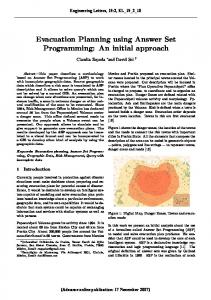
Abstract Currently, people involved in protection against disaster situations must make the decisions about preparing and executing evacuation plans for potential causes of disaster. Hence, it would be desirable to develop a system capable of obtaining and analyzing evacuation plans based on knowledge about their particular environment, the geographic data and their own capabilities, and of exchanging information and services with similar systems as well as with persons. A possible formalism used to develop such system could be Answer Set Programming (ASP). ASP is a declarative knowledge representation and logic programming language[14]. ASP represents a new paradigm for logic programming that allows, using the concept of negation as failure, to handle problems with default knowledge and produce non-monotonic reasoning. Specifically, the objective of our work is to investigate and evaluate the capabilities of Answer Set Programming to represent disaster situations in order to give support in defining evacuation plans. The motivation of our work is based on the idea that ASP posses most of the capabilities that would be desirable that such system should have: It is possible translate geographic information into a format that ASP can handle. There exists Answer Set Planning that provides a natural and elegant way to model planning problems [16]. ASP uses the concept of negation as failure that allows us to express exceptions and represent incomplete knowledge. In ASP there exist different approaches to express
preferences. ASP allows to express restrictions. In order to investigate and evaluate the capabilities of ASP to represent disaster situations we studied the format of geographic information. Based in our own experience we introduce a procedure to construct the hazard zone background knowledge from non spatial part of the geographic information. Normally, in a zone in risk there is a set of pre-defined evacuation routes. However, in a real case it is possible that part of the pre-defined evacuation routes become blocked. In this case definition of alternative evacuation plans are needed. We use Consistency Restoring rules (CR-rules) in order to obtain the alternative evacuation plans. We also prove that programs with CR-rules can be properly represented using ordered disjunction logic programs (ODLP). The alternative evacuation routes obtained using CR-rules do not consider any other characteristic of the path that they follow. Hence, we propose to use language PP in order to express preferences at different levels over the alternative plans. We also define PP par language, as an extension of PP language where the connectives allow to represent compactly preferences having a particular property. Additionally, we present a brief overview about the relationship between language PP and propositional Linear Temporal Logic (LT L), since we consider that language PP could take advantage of the working framework of LT L to express preferences. We also propose an extension of ODLP to a wider class of logic programs. Moreover, we show that in particular extended ordered rules with negated negative literals could be useful to allow a simpler and easier encoding of obtaining the preferred plans w.r.t preferences expressed in PP. Finally, we introduce the notion of Semantic Contents of a program as an alternative point of view to obtain different answer set semantics of a program. One of them is a new semantics introduced in this work, called partial answer sets.
Chapter 1 Resumen en Espa˜ nol 1.1
Introducci´ on
Actualmente, los responsables de la protecci´on contra situaciones de desastre deben tomar decisiones sobre la preparaci´on y ejecuci´on de los planes de evacuaci´on considerando causas potenciales de desastre. Por lo tanto, ser´ıa deseable desarrollar un sistema capaz de obtener y de analizar los planes de la evacuaci´on. Donde este sistema este basado en el conocimiento sobre su ambiente particular, los datos geogr´aficos y sus propias capacidades. Adem´as, debe ser capaz de intercambiar informaci´on y servicios con sistemas similares as´ı como con las personas. Un formalismo que proponemos para desarrollar tal sistema es Answer Set Programming (ASP). ASP es un lenguaje de programaci´on l´ogico y declarativo para la representaci´on del conocimiento [14]. ASP representa un nuevo paradigma para la programaci´on l´ogica que permite, manejar problemas con conocimiento por defecto y razonamiento no-monot´onico mediante con el concepto de la negaci´on como falla. Espec´ıficamente, el objetivo de nuestro trabajo es investigar y evaluar las capacidades de ASP para representar situaciones del desastre con el objetivo de dar ayuda en la definici´on de planes de evacuaci´on. La motivaci´on de nuestro trabajo se baso
1
en la idea que ASP cuanta con muchas de las capacidades que tal sistema debe tener: Es posible traducir la informaci´on geogr´afica a un formato que ASP pueda manejar. Existe Answer Set Planning que proporciona una manera natural y elegante de modelar los problemas de planificaci´on [16]. ASP utiliza el concepto de negaci´on como falla que permite expresar excepciones, restricciones y representar conocimiento incompleto. Adem´as en ASP existen diversos enfoques para expresar preferencias. Para lograr nuestro objetivo, comenzamos estudiando el formato de la informaci´on geogr´afica. Basados en nuestra propia experiencia proponemos un procedimiento para extraer el conocimiento necesario para representar la zona del peligro a partir de la informaci´on geogr´afica. Adem´as consideramos que normalmente en una zona en riesgo hay un conjunto de rutas de evacuaci´on predefinidas. Sin embargo, en un caso real es posible que parte de estas rutas predefinidas se bloqueen. En este caso la definici´on de planes de evacuaci´on alternativos es necesaria. Utilizamos Reglas para restaurar consistencia (reglas-RC) para obtener los planes de evacuaci´on alternativos. Tambi´en mostramos que los programas con reglas-RC se pueden representar correctamente usando programas con disyunci´on ordenada (ODLP). Utilizamos el Lenguaje PP para expresar preferencias a diversos niveles sobre los planes alternativos. Definimos el lenguaje PP par , como extensi´on del lenguaje PP donde sus conectivos permiten que representemos de forma compacta las preferencias que tienen una caracter´ıstica en particular. Adem´as, en este trabajo presentamos una breve descripci´on sobre la relaci´on entre la lenguaje PP y la l´ogica lineal proposicional temporal (LT L), puesto que consideramos que el lenguaje PP podr´ıa tomar ventaja del marco de trabajo de LT L para expresar preferencias. Tambi´en desarrollamos una extensi´on de ODLP a una clase m´as amplia de programas l´ogicos. Es importante mencionar que un subconjunto de estos programas son u ´tiles para permitir una codificaci´on m´as simple y m´as f´acil de obtener los planes 2
preferidos con respecto a las preferencias expresadas en PP. Finalmente, introducimos la noci´on de Contenido Sem´antico de un programa como un punto de vista alternativo para obtener variantes de la sem´antica de Answer Sets. Una de estas variantes es una nueva sem´antica que introducimos en este trabajo, llamada answer sets parciales.
1.2 1.2.1
Antecedentes Answer Set Programming
El uso de Answer Set Programming (ASP) permite describir un problema computacional como un programa l´ogico cuyos answer sets corresponden a las soluciones de problema dado. En este trabajo, un programa es interpretado como una teor´ıa proposicional y la u ´nica negaci´on usada es la negaci´ on como falla. Para lectores no familiarizados con este enfoque, recomendamos [38, 33] como lectura posterior. Por lo tanto nuestra discusi´on se limita a programas proposicionales. Usamos el lenguaje de la l´ogica proposicional de la manera usual, donde los s´ımbolos proposicionales son p, q, . . . ; los conectivos proposicionales son ∧, ∨, →, ⊥, y los s´ımbolos auxiliares son (, ). Una f´ ormula proposicional bien formada es definida inductivamente como sigue: Un s´ımbolo proposicional es una f´ormula proposicional bien formada. Si f y g son f´ormulas proposicionales bien formadas, entonces tambi´en lo son ¬f , f ∧g, f ∨g, f → g. Una f´ormula proposicional bien formada puede ser llamada s´olo f´ ormula. Un atomo es un s´ımbolo proposicional. Dada cualquier f´ormula bien formada f , asumimos ´ que ¬f es exactamente la abreviaci´on de f → ⊥ y > es la abreviaci´on de ⊥ → ⊥. Hacemos ´enfasis en que la u ´nica negaci´on usada en este trabajo es la negaci´ on como falla y es representada por el s´ımbolo ¬. Vale la pena mencionar que siempre es posible manejar la otra negaci´on llamada cl´ asica o tambi´en negaci´ on fuerte, denotada por
3
−, por medio de transformar los ´atomos con negaci´on cl´asica [15]. Cada ´atomo con negaci´on cl´asica, −a, que ocurre en la formula es sustituido por un nuevo ´atomo, a◦ , y la regla ¬(a ∧ a◦ ) es agregada. La regla ¬(a ∧ a◦ ) puede tambi´en ser escrita como (a ∧ a◦ ) → ⊥ basada en el hecho de que ¬f es solo una abreviaci´on de f → ⊥. La firma de un programa P , denotada como LP , es el conjunto de ´atomos que ocurren en P . Una literal es cualquier ´atomo p (una literal positiva) o la negaci´on de un ´atomo ¬p (una literal negativa). Una literal negada es el signo de negaci´on ¬ seguido por una literal, i.e. ¬p or ¬¬p. En particular, f → ⊥ es llamada restricci´ on y tambi´en es denotada como ← f . Una teor´ıa regular o programa l´ogico es solo un conjunto de formulas bien formadas, y puede ser llamado solamente teor´ıa o programa cuando no surjan ambig¨ uedades. En algunas definiciones usamos l´ogica intuicionista, la cual ser´a denotada por I. Para un conjunto dado de ´atomos M y un programa P , escribiremos P `I M para abreviar [27] para toda a ∈ M . Para un conjunto dado de ´atomos M y un programa P , escribiremos P °I M para denotar que: P `I M y que P es consistente con respecto a I (es decir, que no hay una formula A tal que P `I A y P `I ¬A). Algunas veces escribiremos ` en lugar de `I cuando no surjan ambig¨ uedades. Ahora definimos los answer sets (o modelos estables) de programas l´ogicos. La sem´antica de answer sets fue primero definida en t´erminos de la as´ı llamada reducci´ on Gelfond-Lifschitz [14] donde es estudiada en el contexto de transformaciones sobre el programa dependientes de la sintaxis. Nosotros seguimos un enfoque alternativo estudiado por Pearce [38] y tambi´en estudiado por Osorio et.al. [33]. Este enfoque caracteriza los answer sets de una teor´ıa proposicional en t´erminos de l´ogica intuicionista y es presentada en el siguiente teorema. La notaci´on est´a basada en [33]. Theorem 1.1. Sea P una teor´ıa y M un conjunto de ´atomos. M es un answer set
4
para P sii P ∪ ¬(LP \ M ) ∪ ¬¬M °I M . Como notaci´on adicional que ser´a utilizada en el resto de este trabajo tenemos lo siguiente: Un conjunto finito de formulas P es consistente [27] si no hay alguna formula A tal que A y ¬A sean teoremas de P . Un conjunto finito de formulas P es completo [27] si, para cualquier formula A de P , P ` A o P ` ¬A. Un conjunto finito de formulas P 0 es una extensi´ on de un conjunto finito de formulas P [27] si cada teorema de P es un teorema de P 0 . Dados dos conjuntos X y Y , escribimos X ⊂ Y para denotar que X ⊆ Y and X 6= Y . Como de costumbre en Answer Set Programming, consideramos que un programa con s´ımbolos del predicado es solamente una abreviatura del programa sin variables, denotado como sinV ariables(P ). En algunos casos, necesitamos modelar algunos problemas usando s´ımbolos del predicado con variables, donde estas variables deben ser instanciadas solamente con un subconjunto del universo de Herbrand del programa. Esta clase de programas se llama programas de clases con s´ımbolos de predicado [4]. Por ejemplo, utilizaremos programas de clases con s´ımbolos de predicado cuando estudiamos la codificaci´on de un problema de planificaci´on en la secci´on 1.2.4. Actualmente, hay varios resolvedores para Answer Sets. En este trabajo hemos usado DLV1 , SMODELS2 , un frontend para DLV llamado DLVK3 , una modificaci´on de SMODELS que puede ser usada para obtener los answer sets preferidos bajo la sem´antica de Disyunci´on Ordenada llamado PSMODELS, y el Logics Workbench (LWB)4 que nos permite trabajar con l´ogica Intucionista [38]. 1 2 3 4
http://www.dbai.tuwien.ac.at/proj/dlv/ http://www.tcs.hut.fi/Software/smodels/ http://www.dbai.tuwien.ac.at/proj/dlv/K/ http://www.lwb.unibe.ch/about/index.html
5
1.2.2
Programas-RC y Programas Abductivos
Las reglas para restaurar consistencia (reglas-RC) son las reglas que se agregan a los programas l´ogicos disyuntivos est´andares, pero se aplican solamente cuando las reglas regulares (las reglas est´andar) en el programa conducen a inconsistencia. Una regla+
RC es escrita como α ← β, lo cual se lee intuitivamente como: Si el programa es inconsistente, entonces asumimos α ← β. En otro caso, ignore la regla. Recordamos el siguiente ejemplo presentado en [3], puesto que ilustra claramente el uso de las reglasRC. En este ejemplo r1 denota el nombre de la regla-RC. a ← ¬b. ¬ a. +
r1 : b ← . Las primeras dos reglas son reglas regulares y la tercera regla es una regla-RC. Esta clase de programas ser´a llamada CR-programas. Podemos ver que el programa sin la regla-RC es inconsistente. Sin embargo, si la regla-RC se utiliza entonces se restaura la consistencia, as´ı el answer set {¬a, b} es obtenido. La sem´antica de los programas-RC se define en t´erminos de los answer sets m´ınimos generalizados. En [3] los autores dan una traducci´on de programas-RC a programas l´ogicos abductivos, que llaman hard reduct, y la sem´antica se define como los answer sets m´ınimos generalizados del hard reduct del programa. Las definiciones siguientes se encuentran en [3]: Definition 1.1. [3] Un programa l´ogico abductivo es un par hP, Ai donde P es un programa arbitrario y A un conjunto de ´atomos, llamado abducibles. Definition 1.2. [3] Sea hP, Ai programa l´ogico abductivo y ∆ ⊆ A. Decimos que M (∆) es un answer set generalizado de P con respecto a A sii M (∆) es un answer set de P ∪ ∆. 6
Definition 1.3. [3] Sean M (∆1 ) y M (∆2 ) dos answer sets generalizados de P con respecto a A. Definimos M (∆1 ) < M (∆2 ) sii ∆1 ⊂ ∆2 (orden por inclusi´on de conjuntos). Definition 1.4. Sea P un programa y sea A un conjunto de ´atomos. M (∆) es un answer set m´ınimo generalizado de P con respecto a A y el orden < sii M (∆) es un answer set generalizado de P y es m´ınimo con respecto al orden por inclusi´on de conjuntos. Finalmente, el ejemplo siguiente ilustra c´omo la sem´antica de los programas-RC se define en t´erminos de los answer sets m´ınimos generalizados. Example 1.1. Sea P1 = {p ← ¬q. r ← ¬s. q ← t. s ← t. ← p, r} el programa del Ejemplo 4 introducido en [3]. Podemos ver que el programa P1 no tiene answer sets. Sin embargo, para restaurar consistencia, podemos definir un Programa-RC que agrega algunas reglas-RC. Por ejemplo, definamos el Programa-RC P10 = P 1 ∪ CR1 donde +
+
+
CR1 = {r1 : q ←, r2 : s ←, r3 : t ←}. Como mencionamos, la sem´antica de P10 est´a definida en t´erminos de los answer sets m´ınimos generalizados. Entonces, traduciendo P10 en un programa l´ogico abductivo obtenemos hP1 , Ai donde el conjunto de abducibles es A = {q, s, t}. Podemos verificar que los answer sets m´ınimos generalizado de P1 son {q, r}, {s, p} y {t, q, s}.
1.2.3
Programas L´ ogicos con Disyunci´ on Ordenada
En [7], Brewka introdujo los Programas L´ogicos con Disyunci´on Ordenada, abreviados como LPODs. Para definir esta clase de programas, el conectivo ×, llamado disyunci´on ordenada, se agrega al sistema de conectivos para f´ormulas proposicionales presentados en la Secci´on 1.2.1. La intuici´on detr´as de los LPODs es expresar conocimiento por falla 7
con conocimiento sobre preferencias de una manera simple y elegante [9]. Como hemos mencionado en la Secci´on 1.2.1, en este trabajo estamos considerando solamente un tipo de negaci´on, negaci´on como falla, pero esto no afecta la validez de los resultados dados en [7]. Formalmente, un programa l´ogico con disyunci´on ordenada es un conjunto de reglas de la forma: C1 × . . . × Cn ← A1 , . . . , Am , ¬B1 , . . . , ¬Bk
(1.1)
donde Ci , Aj y Bl son todos ´atomos sin varables. C1 . . . Cn son normalmente llamados las opciones de una regla y su lectura intuitiva es la siguiente: Si el cuerpo es verdadero y C1 es posible, entonces C1 ; si C1 no es posible, entonces C2 ; . . . ; si ninguno de C1 , . . . , Cn−1 es posible entonces Cn . Algunos casos especiales se pueden precisar, n = 0 (restricciones), n = 1 (programas extendidos), m = k = 0 (hechos). La sem´antica de los programas l´ogico con disyunci´on ordenada ser´a presentada en la Secci´on 1.3.1 donde una extensi´on de los programas l´ogicos con disyunci´on ordenada se presenta. Actualmente, hay una modificaci´on de SMODELS5 que se puede utilizar para el c´alculo del los answer set preferidos de los programas l´ogicos con disyunci´on ordenada llamada PSMODELS6 [9].
1.2.4
Planificaci´ on en Answer Sets
En un problema del planificaci´on, estamos interesados en buscar una secuencia de acciones que conduzca de un estado inicial dado a un estado que define la meta. Para especificar totalmente un problema del planificaci´on, necesitamos indicar que acciones se permiten en un plan. La planificaci´on en Answer Sets usa lenguajes de acciones para especificar los efectos de acciones y en particular son usados para modelar problemas 5 6
http://www.tcs.hut.fi/Software/smodels/ http://www.tcs.hut.fi/Software/smodels/priority/
8
de planificaci´on [16]. Algunos de estos lenguajes de acci´on son A, B, y C [16]. Por otra parte, un problema del planificaci´on especificado en estas clases de lenguajes tiene una codificaci´on natural y f´acil en Answer Set Programming. Languaje A. El alfabeto del lenguaje A consiste de dos conjuntos no vac´ıos y disjuntos de s´ımbolos F llamado el conjunto de fluentes, y A llamado el conjunto de acciones. Intuitivamente, un fluente expresa una caracter´ıstica de un objeto en un mundo, y forma parte de la descripci´on de los estados del mundo. Una literal fluente es un fluente o un fluente precedido por ∼. Un estado σ es un conjunto de fluentes. Decimos que un fluente f se cumple en un estado σ si f ∈ σ. Decimos que un fluente literal ∼ f se cumple en σ si f 6∈ σ. Cuando las acciones son ejecutadas exitosamente cambian el estado del mundo. Las situaciones son representaciones de la historia de la ejecuci´on de acciones. La situaci´on inicial [an , . . . , a1 ] corresponde a la historia donde la acci´on a1 se ejecuta en la situaci´on inicial, seguida por a2 , y as´ı hasta an . Hay una relaci´on simple entre situaciones y estados. En cada situaci´on s algunos fluentes son verdaderos y algunos otros son falsos. El lenguaje A se puede dividir en tres sub-languajes: lenguaje para descripci´ on del dominio, lenguaje de observaci´on y lenguaje de consulta. Dado un problema del planificaci´on, ´este puede ser expresado en una lenguaje de acciones por medio de un triple (D, O, G) tal que D es la descripci´on del dominio, O es el conjunto de observaciones y G es el conjunto de condiciones de la meta. Por otra parte, es posible definir una codificaci´on en Answer Sets de este problema de planificaci´on especificado en un lenguaje de acciones, denotada como π(D, O, G, l), donde l es un n´ umero entero positivo que corresponde a la longitud del plan, es decir, el n´ umero de las acciones que se deben realizar para alcanzar la meta. Entonces, es posible obtener la soluci´on del problema de planificaci´on (los planes) de los answer sets de π(D, O, G, l). La idea b´asica es que decidimos sobre una longitud 9
del plan l para enumerar ocurrencias de las acciones hasta los puntos del tiempo que corresponden a esa longitud, y codificar las metas como restricciones acerca del tiempo l + 1, tales que los answer sets que codifican las ocurrencias de las acciones que no satisfacen la meta en el tiempo l + 1 son eliminados. As´ı cada uno de los answer sets que sobreviven a las restricciones corresponde a un plan. Es importante mencionar que en la codificaci´on en Answer Sets de los problemas de planificaci´on expresados en lenguaje A, si f es un literal fluente negativa ∼ g entonces f ser´a codificada como neg(g), donde, neg(g) corresponde la negaci´on cl´asica. Los detalles de estos sublenguajes y c´omo obtener la codificaci´on de un problema del planificaci´on de una especificaci´on en un lenguaje de acciones pueden encontrarse en [16, 4]. Presentamos solamente un ejemplo que muestra c´omo especificar el problema simple del planeaci´on del mundo de los bloques en lenguaje A que proviene de [4]. Example 1.2. El problema de planificaci´on de los cubos puede ser expresado en lenguaje A como sigue: 1. Clase: block(X). En el resto de este ejemplo, X y Y var´ıan en la clase block. 2. Fluentes: on(X, Y ), ontable(X), clear(X), holding(X), handempty 3. Acciones: pick up(X), put down(X), stack(X, Y ), unstack(X, Y ) 4. Condiciones de ejecuci´on, denotadas por D: executable pick up(X) if clear(X), ontable(X), handempty. executable put down(X) if holding(X). executable stack(X, Y ) if holding(X), clear(Y ). executable unstack(X, Y ) if clear(X), on(X, Y ), handempty. 5. Proposiciones de efecto. pick up(X) causes ∼ ontable(X), ∼ clear(X), holding(X), ∼ handempty. 10
put down(X) causes ontable(X), clear(X), ∼ holding(X), handempty. stack(X, Y ) causes ∼ holding(X), ∼ clear(Y ), clear(X), handempty, on(X, Y ). unstack(X, Y ) causes holding(X), clear(Y ), ∼ clear(X), ∼ handempty, ∼ on(X, Y ). 6. Considerando la clase block como {a, b, c, d} las condiciones iniciales, denotadas por I, son descritas como: initially(clear(a)). initially(clear(c)). initially(clear(d)). initially(handempty). initially(ontable(c)). initially(ontable(b)). initially(on(a, b)). initially(on(d, c)). 7. Las condiciones de meta, denotadas por G, son el conjunto de literales {on(a, c), on(c, b), ontable(d)}. El Lenguaje B resulta cuando el Lenguaje A es extendido para permitir proposiciones de causa est´aticas. Usando proposiciones de causa est´aticas podemos expresar conocimiento acerca de los estados en base a los estados que son posibles o validos. Este conocimiento puede ser usado indirectamente para inferir efectos de acciones, ejecutabilidad de las acciones o ambas. M´as detalles acerca de proposiciones de causa est´aticas y codificaci´on de problemas expresados en Lenguaje B pueden ser encontrados en [16, 4].
1.2.5
Un lenguaje para preferencias de planes: Lenguaje PP
El lenguaje PP [43] permite la especificaci´on de preferencias del usuario. Ademas PP cuenta con una implementaci´on en programaci´on l´ogica, basada en Answer Set Programming. El lenguaje PP permite especificar preferencias entre posibles planes y tambi´en preferencias temporales sobre los planes. Las preferencias que representan tiempo son expresadas usando los conectivos temporales next, always, until y eventually. Hay tres clases de preferencias en PP [43] deseos b´asicos, preferencias at´omicas y preferencias generales . En este trabajo estudiamos las dos primeras clases de preferencias 11
porque ellas fueron u ´tiles para expresar preferencias en los planes de evacuaci´on. Un deseo b´asico, denotado como ϕ, es una f´ormula de PP que expresa una preferencia sobre una trayectoria con respecto a la ejecuci´on de una cierta acci´on o con respecto a los estados que la trayectoria llega cuando se ejecuta una acci´on. Una preferencia at´omica representa un orden entre f´ormulas de deseo b´asico. Indica que las trayectorias que satisfacen ϕ1 son preferibles a los que satisfagan ϕ2 , etc. Claramente, las f´ormulas de deseo b´asico son casos especiales de las preferencias at´omicas.
1.3
Contribuci´ on
Recordemos que el objetivo de nuestro trabajo es investigar y evaluar las capacidades de Answer Set Programming para representar situaciones del desastre con el fin de apoyar en la definici´on de planes de la evacuaci´on. Para ello comenzamos a analizar c´omo la informaci´on geogr´afica de la zona de desastre a modelar se puede traducir a un formato que Answer Sets es capaz de manejar. Continuamos estudiando y aplicando diversos enfoques en Answer Sets que son u ´tiles para definir los planes de la evacuaci´on, tales como, Programas-RC, Programas L´ogicos con Disyunci´on Ordenada, planificaci´on en Answer Sets, el lenguaje para preferencias de planes y los answer sets m´ınimos generalizados. Espec´ıficamente, definimos la extensi´on de Programas L´ogicos con Disyunci´on Ordenada y vimos su utilidad. Ademas se presento c´omo y porqu´e los enfoques en Answer Sets mencionados se aplican para definir planes de la evacuaci´on y tambi´en se presentaron algunas debilidades de estos enfoques que este trabajo trata.
12
1.3.1
Programas L´ ogicos con Disyunci´ on Ordenada Extendidos
En [7] la cabeza de las reglas con disyunci´on ordenada es definida en t´erminos de literales sin variables. En esta secci´on, la cabeza y el cuerpo para reglas con disyunci´on ordenada extendidas son definidos en t´erminos de formulas porposicionales bien formadas. Consideramos que una sintaxis m´as amplia para estas reglas podr´ıa darnos algunas ventajas. Por ejemplo, el uso de expresiones jerarquizadas podr´ıa simplificar la tarea de escribir programas l´ogicos y mejorar su legibilidad puesto que podr´ıa permitirnos escribir reglas m´as cortas y de una manera m´as natural. Definition 1.5. Una regla con disyunci´on ordenada extendida es una formula proposicional bien formada como se defini´o en la Secci´on 1.2.1, o una formula de la forma: f1 × . . . × fn ← g donde f1 , . . . , fn , g son formulas proposicionales bien formadas.
(1.2) Un programa con
disyunci´ on ordenada extendido es un conjunto finito de reglas con disyunci´on ordenada extendida. Las f´ormulas f1 . . . fn generalmente son llamadas las opciones de una regla y su lectura intuitiva es como sigue: si el cuerpo es verdadero y f1 es posible, entonces f1 ; si f1 no es posible, entonces f2 ; . . . ; si ninguno de f1 , . . . , fn−1 es posible entonces fn . El caso particular donde toda fi es una literal y g es una conjunci´on de literales corresponde a los programas con disyunci´on ordenada originales seg´ un lo presentado por Brewka en [7], y que llamaremos programas con disyunci´on ordenada est´andar. Recordamos que los programas con disyunci´on ordenada est´andar de Brewka utilizan el conectivo para la negaci´on fuerte.
13
Aqu´ı consideraremos solamente un tipo de negaci´on (negaci´on como falla) pero esto no afecta los resultados dados en [7]. Si n = 0 la regla es adem´as una restricci´on, es decir, ⊥ ← g. Si n = 1 es una regla extendida y si g = > la regla es un hecho y se puede escribir como f1 × . . . × fn . Ahora, presentamos la sem´antica de los programas con disyunci´on ordenada extendidos. La mayor´ıa de las definiciones presentadas aqu´ı se toman de [7, 9]. Definition 1.6. [7]Sea r := f1 × . . . × fn ← g una regla con disyunci´on ordenada extendida. Para 1 ≤ k ≤ n la k-´esima opci´ on de r es definida como sigue: rk := (fk ← g, ¬f1 , . . . ¬fk−1 ). Definition 1.7. [7] Sea P un programa con disyunci´on ordenada extendido. P 0 es un programa particionado de P si es obtenido por reemplazar cada regla r := (f1 × . . . × fn ← g) en P por una de sus opciones r1 , . . . , rk . M es un answer set de P sii es un answer set7 de un programa particionado P 0 de P . Definition 1.8. [7]Sea M un answer set de un programa con disyunci´on ordenada extendido P y sea r := (f1 × . . . × fn ← g) una regla de P . Definimos el grado de satisfacci´ on de r con respecto a M, denotado por degM (r), como sigue: —si M ∪ ¬(LP \ M ) 6`I g, entonces degM (r) = 1. — si M ∪ ¬(LP \ M ) `I g entonces degM (r) = min1≤i≤n {i | M ∪ ¬(LP \ M ) `I fi }. El teorema siguiente indica la relaci´on entre los answer sets de un programa con disyunci´on ordenada extendido y el grado de satisfacci´on de cada regla en el programa. Theorem 1.2. [7] Sea P un programa con disyunci´on ordenada extendido. Si M es un answer set of P entonces M satisface todas las reglas en P con alg´ un grado. 7
Notemos que debido a que no estamos considerando negaci´on fuerte, no hay posibilidad de tener answer sets inconsistentes.
14
Definition 1.9. [9] Sea P un programa con disyunci´on ordenada extendido y M un i conjunto de literales. Definimos SM (P ) = {r ∈ P | degM (r) = i}.
Con las definiciones anteriores introdicumos dos tipos diferentes de relaciones de preferencia entre los answer sets de un programa con disyunci´on ordenada extendido: preferencia basada en inclusi´on de conjuntos y preferencia basada en la cardinalidad de conjuntos. Definition 1.10. [9] Sea M y N answer sets de un programa con disyunci´on ordenada extendido P . Entonces decimos que M es preferido por inclusi´on a N , denotado como j j i i M >i N , sii hay un i tal que SN (P ). (P ) ⊂ SM (P ) = SN (P ) y para todo j < i, SM
Decimos que M es preferido por cardinalidad a N , denotado como M >c N , sii hay un ¯ ¯ ¯ j ¯ j i i i tal que |SM (P )¯. (P )| > |SN (P )¯ = ¯SN (P )| y para todo j < i, ¯SM Definition 1.11. [9] Sea M un answer set de un programa con disyunci´on ordenada extendido P . M es un answer set preferido por inclusi´on de P si no hay alg´ un answer set M 0 de P , M 6= M 0 , tal que M 0 >i M . M es un answer set preferido por cardinalidad de P si no hay M 0 answer set de P , M 6= M 0 , tal que M 0 >c M .
1.3.2
Answer Set M´ınimos Generalizados y Disyunci´ on Ordenada
Ahora, definimos una caracterizaci´on de los answer set m´ınimos generalizados de un programa en t´erminos de un programa con disyunci´on ordenada est´andar. Este resultado te´orico prueba que ambos programas abductivos y los programas con reglas-RC se pueden representar correctamente usando disyunci´on ordenada. Definition 1.12. Sea hP, Ai un programa l´ogico abductivo. Entonces, definimos una traducci´on a un programa con disyunci´on ordenada est´andar, denotado por ord(P, A), 15
como sigue: Primero, para alguna literal a ∈ A la regla ra es definida como a• × a, donde a• es una literal que no ocurre en el programa original. Definimos ord(P, A) = P ∪ {ra | a ∈ A}. Lemma 1.1. M ∩ LP es un answer set generalizado del programa l´ogico abductivo hP, Ai sii M es un answer set de ord(P, A). El teorema siguiente prueba la validez de nuestra traducci´on para la sem´antica de programa l´ogicos abductivos. Theorem 1.3. Sea hP, Ai un programa l´ogico abductivo y M un conjunto de ´atomos. M ∩LP es un answer set m´ınimo generalizado de hP, Ai sii M es un answer set preferido por inclusi´on de ord(P, A).
1.3.3
Preferencias en t´ erminos de programas con Disyunci´ on Ordenada Extendidos
Podemos especificar un orden entre los answer sets de un programa con disyunci´on ordenada extendido con respecto a una lista de ´atomos. Definition 1.13. Sea P un programa normal. Sean M y N dos answer sets de P . Sea C = [c1 , c2 , . . . , cn ] un conjunto ordenado de formulas. El answer set M es preferido al answer set N con respecto a C ∪ P (denotado como M i N , si et seulement si il y a un i tel que SN (P ) ⊂ SM (P ) et pour tout j j (P ). Nous disons que M est pr´ef´er´e par cardinalit´e `a N , indiqu´e (P ) = SN j < i, SM i i comme M >c N , si et seulement si il y a un i tel que |SM (P )| > |SN (P )| et pour tout ¯ j ¯ ¯ j ¯ j < i, ¯SM (P )¯ = ¯SN (P )¯.
Definition 2.11. [9] Etant donn´e M un answer set d’un programme avec disjonction ordonn´ee ´etendue P . M est un answer set pr´ef´er´e par inclusion de P s’il n’y a aucun answer set M 0 de P , M 6= M 0 , tel que M 0 >i M . M est un answer set pr´ef´er´e par cardinalit´e de P s’il n’y a pas M 0 answer set de P , M 6= M 0 , tel que M 0 >c M .
2.3.2
Answer Set Minimum G´ en´ eralis´ e et Disjonction ordonn´ ee
Nous proposons maintenant une caract´erisation des answer sets minimums g´en´eralis´es d’un programme en terme de programme avec disjonction ordonn´ee standard. Ce r´esultat th´eorique prouve que les deux programmes abductifs et les programmes avec CR-r`egles peuvent ˆetre repr´esent´es correctement en utilisant la disjonction ordonn´ee.
38
Definition 2.12. Etant donn´e < P, A > un programme logique abductif. Alors, nous d´efinissons une traduction `a un programme avec disjonction ordonn´ee standard, indiqu´e par ord(P, A), comme suit : D’abord pour un litt´eral a ∈ A la r`egle ra est d´efinie comme a• × a, o` u a• est un litt´eral qui n’apparaˆıt pas dans le programme original. Nous d´efinissons ord(P, A) = P ∪ {ra | a ∈ A}. Lemma 2.1. M ∩ LP est un answer set g´en´eralis´e du programme logique abductif < P, A > si et seulement si M est un answer set de ord(P, A). Le th´eor`eme suivant prouve la validit´e de notre traduction pour la s´emantique de programmes logiques abductifs. Theorem 2.3. Etant donn´e < P, A > un programme logique abductif et M un ensemble d’atomes. M ∩ LP est un answer set minime ou g´en´eralis´e de < P, A > si et seulement si M est un answer set pr´ef´er´e par inclusion de ord(P, A).
2.3.3
Pr´ ef´ erences en termes de programme avec Disjonction ´ Ordonn´ ee Etendue
Nous pouvons sp´ecifier un ordre entre les answer sets d’un programme avec disjonction ordonn´ee ´etendue relative `a une liste d’atomes. Definition 2.13. Etant donn´e P un programme normal. Etant donn´e M et N deux answer sets de P . Etant donn´e C = [c1 , c2 , . . . , cn ] un ensemble ordonn´e de formules. L’answer set M est pr´ef´er´e `a l’answer set N respectivement `a C ∪ P (indiqu´e comme M i N , iff there is an i j j i i such that SN (P ) ⊂ SM (P ) and for all j < i, SM (P ) = SN (P ).
CHAPTER 6. EXTENDED ORDERED DISJUNCTION PROGRAMS
106
Example 6.4. If we consider the extended ordered program P from Example 6.1 and the results from Example 6.3, then we can verify that M1 is inclusion preferred to M2 and 1 1 1 1 (P ). (P ) ⊂ SM to M3 , i.e., M1 >i M2 and M1 >i M3 since SM (P ) ⊂ SM (P ) and SM 3 1 1 2
Definition 6.8. [9] Let M and N be answer sets of an extended ordered program P . Then we say that M is cardinality preferred to N , denoted as M >c N , iff there is an ¯ j ¯ ¯ j ¯ i i i such that |SM (P )| > |SN (P )| and for all j < i, ¯SM (P )¯ = ¯SN (P )¯. Example 6.5. If we consider the extended ordered program P from Example 6.1 and the results from Example 6.3, then we can verify that M2 is cardinality preferred to 2 2 1 1 M3 , i.e., M2 >c M3 since |SM (P )| > |SM (P )| and |SM (P )| = |SM (P )|. 2 3 2 3
We also can verify that M1 is cardinality preferred to M2 and to M3 , i.e., M1 >c M2 1 1 1 1 and M1 >c M3 since |SM (P )| > |SM (P )| and |SM (P )| > |SM (P )|. 1 2 1 3
Definition 6.9. [9] Let M be an answer set of an extended ordered program P . M is an inclusion preferred answer set of P if there is no answer set M 0 of P , M 6= M 0 , such that M 0 >i M . Definition 6.10. [9] Let M be an answer set of an extended ordered program P . M is a cardinality preferred answer set of P if there is no M 0 answer set of P , M 6= M 0 , such that M 0 >c M . Example 6.6. If we consider the extended ordered program P from Example 6.1, the results from Example 6.3, Example 6.4 and Example 6.5 then we can verify that M1 is the inclusion preferred answer set of P and the cardinality preferred answer set of P.
CHAPTER 6. EXTENDED ORDERED DISJUNCTION PROGRAMS
6.2
107
Translation from an abductive logic program to a standard ordered disjunction program
In Section 4.7 we reviewed CR-programs. We saw that the semantics of a CR-program is defined in terms of the minimal generalized answer sets of a particular abductive logic program. This abductive logic program is based on the original program and a set of abducibles which corresponds to a subset of the signature of this original program. In this section, we propose a characterization of minimal generalized answer sets in terms of ordered disjunction programs. This theoretical result proves that both abductive programs and programs with CR-rules can be properly represented using ordered disjunction. Definition 6.11. Let < P, A > be an abductive logic program. Then we define a translation into a standard ordered program, denoted by ord(P, A), as follows: First, for any literal a ∈ A the clause ra is defined as a• × a, where a• is a literal that does not occur in the original program. We define ord(P, A) = P ∪ {ra | a ∈ A}. Lemma 6.1. M ∩LP is a generalized answer set of the abductive logic program < P, A > iff M is an answer set of ord(P, A). Sketch. Let P(A) be all subsets of A and RP(A) := {rl1 | l ∈ A \ P(A)}∪{rl2 | l ∈ P(A)}. Let us recall that rl = l• × l so that rl1 = l• and rl2 = l ← ¬l• . The proof follows from the fact that all P ∪ RP(A) correspond exactly to the split programs of ord(P, A). The next theorem proves the validity of our ordered translation for the semantics of abductive logic programs when it uses set inclusion. Theorem 6.2. Let < P, A > be an abductive program and M a set of atoms. M ∩ LP is a minimal generalized answer set of < P, A > iff M is an inclusion preferred answer set of ord(P, A).
CHAPTER 6. EXTENDED ORDERED DISJUNCTION PROGRAMS
108
Sketch. It is only needed to prove that M ∩ LP is minimal w.r.t. abductive inclusion/cardinality order iff M is minimal w.r.t. inclusion/cardinality preferred order. The proof is straightforward using the fact that for all rules in ord(P, A), which are in the form rules in Definition 6.1, n ≤ 2 implies that g = >. Example 6.7. This example shows how our ordered translation works. It is based on the CR-program P10 from Example 4.11 of Section 4.7. In particular we consider the abductive logic program hP1 , Ai used to obtain the semantics of the CR-program P10 , where P1 is the following program: p ← ¬q. r ← ¬s. q ← t. s ← t. ← p, r. and A = {q, s, t}. According to the translation defined in 6.11 we have that ord(P, A) is the following program: p ← ¬q. r ← ¬s. q ← t. s ← t. ← p, r. q• × q s• × s t• × t Moreover we can verify that the inclusion preferred answer sets o f ord(P, A) are M1 = {q • , q, r}, M2 = {s• , s, p} and M3 = {q • , s• , t• , t, q, s}. Hence, the minimal
CHAPTER 6. EXTENDED ORDERED DISJUNCTION PROGRAMS
109
generalized answer sets of hP1 , Ai are M1 = {q, r}, M2 = {s, p} and M3 = {t, q, s} since LP1 = {p, q, r, s, t} as in Example 4.11.
6.3
Preferences in terms of extended ordered programs with double negation
Preferences are useful when the space of feasible solutions of a given problem is dense but not all these solutions are equivalent w.r.t. some additional requirements. In this case, the goal is to find feasible solutions that most satisfy these additional requirements. In [9] Brewka introduced logic programs with ordered disjunction (LPODs) where the connective ×, called ordered disjunction, allows to express default knowledge with knowledge about preferences in a simple and elegant way. However, if we only want to specify a preference ordering among the answer sets of a program with respect to an ordered set of atoms by means of adding a standard ordered disjunction rule to the original program then, ordered disjunction as defined by Brewka does not work since it corresponds to a disjunction where an ordering is defined. For instance, if P is the following program a←. b ← ¬c. c ← ¬b. d ← ¬a. f ← c, ¬a. e ← b, ¬a. then the answer sets of this program are {a, b} and {a, c}. Now, if we want to specify a preference ordering among the answer sets of a program with respect to the ordered set of atoms [f, c] then we could consider to add to
CHAPTER 6. EXTENDED ORDERED DISJUNCTION PROGRAMS
110
the program P the standard ordered disjunction rule {f × c} that stands for “if f is possible then f otherwise c” (see [7]). Then, thinking in a preference sense, the intuition indicates that the inclusion-preferred answer sets of P ∪ {f × c} should be {a, c}. However, we obtain two inclusion-preferred answer sets {a, b, f } and {a, c, f }. Therefore, in order to specify a preference ordering among the answer sets of a program with respect to an ordered set of atoms, in this section we propose to use a particular set of extended ordered disjunction programs [46]. Specifically, we propose to add to the original program an extended ordered rule such that this rule is defined using the ordered set of atoms and each atom has double default negation. We are going to explain way we propose to use atoms with double default negation. Let us consider ¬¬a where a is an atom. Since ¬¬a is equivalent to the restriction ← ¬a, the intuition behind ¬¬a is to indicate that it is desirable that a holds in the model of a program. Formally, as we defined in Background Section, an atom with double negation corresponds to a negated negative literal where the only negation used is default negation. Hence, if we consider again the previous program P and we want to to specify a preference ordering among the answer sets of P with respect to an ordered set of atoms [f, c] we have to do the following: First we define the extended ordered disjunction rule using the ordered set of atoms [f, c] such that each atom has double default negation, i.e, we define {¬¬f × ¬¬c}. Then, we add this extended ordered disjunction rule to the original program P , i.e., we define the following extended ordered disjunction program: P ∪ {¬¬f × ¬¬c}. As we will prove in the following subsection, we obtain the desired inclusion-preferred answer set {a, c} from this extended ordered disjunction program. We explained that the intuition behind an extended ordered rule using negated negative literals is to indicate that we want to specify a preference ordering among the answer sets of a program with respect to an ordered set of atoms. However, in case that
CHAPTER 6. EXTENDED ORDERED DISJUNCTION PROGRAMS
111
the answer sets of the program do not contain any of the atoms in the given ordered set of atoms then the extended ordered rule must allow to obtain all the answer sets of the program. In order to obtain all the answer sets of the program we propose to add a positive literal to the end of the extended ordered rule that we defined as we explained above. This positive literal must be an atom that does not occur in the original program, for instance the atom all pref . For instance,let us consider again the program P that has the answer sets {a, b} and {a, c}. If we want to specify a preference ordering among the answer sets of this program with respect to the ordered set of atoms C = [f, e] then we define the extended ordered rule as we explained above but we add the atom all pref at the end of the rule, i.e., ¬¬f × ¬¬e × all pref . The new extended ordered rule indicates that we prefer the answer sets where f holds to the answer sets where e holds and if there is no answer sets of the program where f or e holds then all answer sets are preferable. It is worth to mentioning that in case that there is no answer sets of the program where f or e holds then all the answer sets will contain the atom all pref . Hence, the extended ordered program is as follows: a←. b ← ¬c. c ← ¬b. d ← ¬a. f ← c, ¬a. e ← b, ¬a. ¬¬f × ¬¬e × all pref. As we expected, we obtain the inclusion-preferred answer sets: {a, c, all pref } and {a, b, all pref } since there is no answer sets of the program containing f or e. The following short examples also show the role of negated negative literals in an extended ordered program.
CHAPTER 6. EXTENDED ORDERED DISJUNCTION PROGRAMS
112
Example 6.8. If consider the following standard ordered program a×b we can verify that the inclusion preferred answer set of it is {a} since ordered disjunction corresponds to a disjunction where an ordering is defined. However, the following extended ordered program ¬¬a × ¬¬b has no answer sets since the extended ordered rule only indicates that we prefer the answer sets containing a to the answer sets containing b but there is no answer sets. Example 6.9. We also can consider the following standard ordered program, a × b. b ← ¬a we can verify that the inclusion preferred answer set of it is {a} since ordered disjunction corresponds to a disjunction where an ordering is defined. However, the following extended ordered program ¬¬a × ¬¬b b ← ¬a only has {b} as its inclusion preferred answer set, since the extended ordered rule only indicates that we prefer the answer sets containing a to the answer sets containing b and program b ← ¬a has only the answer set {b} . In order to formalize our previous discussion about the specification of an ordering among the answer sets of a normal program with respect to an ordered set of atoms using an extended ordered program, we are going to introduce Lemma 6.7. This lemma
CHAPTER 6. EXTENDED ORDERED DISJUNCTION PROGRAMS
113
allows us to obtain the most preferred answer set of a normal program with respect to an ordered set of formulas in terms of a particular extended ordered program. This particular extended ordered program results from joining the original normal program and a particular ordered disjunction rule that is defined in terms of the ordered set of atoms. It is worth mentioning that the proof of Lemma 6.7 uses other auxiliary lemmas that we are going to present before we present Lemma 6.7. Additionally, we have to mention that most of these auxiliary lemmas are for general purpose. We start introducing a definition and a proposition that allows us to define the most preferred answer set with respect to a program and an ordered set of formulas. Definition 6.12. Let P be a normal program and let M and N be two answer sets of P . Let C = [c1 , c2 , . . . , cn ] be an ordered set of formulas. The answer set M is preferred to the answer set N with respect to C ∪ P (denoted as M |M 0 |, i.e., by definition of partialM odel(∅) of P (Definition 9.3), we have to prove that ∃hS, M 0 i ∈ SC(P )∅ such that M = pos(M 0 ), and @ a M 00 , a partialM odel(∅) of P , such that |M 00 | > |M 0 |. By hypothesis, we have seen that exists hS, M 0 i ∈ SC(P )∅ such that M = pos(M 0 ). We are going to prove by contradiction that @ a M 00 , a partialM odel(∅) of P , such that |M 00 | > |M 0 |. Let M 00 be a partialM odel(∅) of P , such that |M 00 | > |M 0 |. Then
CHAPTER 9. SEMANTIC CONTENTS
191
|M 00 | > |LP | since by hypothesis M 0 is complete, a contradiction. We also want to remark that our definition of partial answer sets is different from the definition of partial stable model semantics introduced in [39] and it is also different from the definition of partial models given in [44]. Using Partial answer sets to restore consistency Now we want to present an example in a planning domain where partial answer sets can be useful. We think that in case that a program has no answer sets, partial answer sets could help to detect the cause of inconsistency. In particular, in planning domains partial answer sets could correspond to partial plans. Then, the idea is to analyze the partial plans and review the possible causes of inconsistency. The following example illustrates this idea presenting a short planing problem. Example 9.8. Somebody plans to submit his/her paper to a congress and present it. Additionally, this person receives an invitation to present his/her paper. Then we can express this problem as a planning problem where there are three fluents: noM oneyP roblems, invitedP aper and inCongress; there are only one action: makeInscription; and the goal is that the person assists to the congress, i. e., the fluent inCongress holds. Then a brief description of the planning problem could be the following:
CHAPTER 9. SEMANTIC CONTENTS
192
% If it is an invitedPaper at time 1 then inCongress holds at time 2 holds(inCongress, 2) ← holds(invitedP aper, 1).
%When action payInscription occurs at time 1 causes inCongress at time 2. holds(inCongress, 2) ← occurs(makeInscription, 1).
%Normally, if there is not evidence about action makeInscription %occurs at time 1 then inCongress does not holds at time 2. holds(neg(inCongress), 2) ← ¬occurs(makeInscription, 1).
%InvitedPaper holds at time 1. holds(invitedP aper, 1).
%If there is no money problems then action makeInscription is possible. occurs(makeInscription, 1) ← holds(noM oneyP roblems, 1). We can verify that the program does not has answer sets, i.e., there is an inconsistency. In order to detect the inconsistency we could analyze the partial answer sets of this program: {holds(invitedP aper, 1), holds(inCongress, 2)} The partial answer set could suggest that there is a contradiction with holds(invitedP aper, 1) or
holds(inCongress, 2).
Then, in order to detect the possible causes of contradiction we could review the program and see that normally, if there is not evidence about action makeInscription occurs at time 1 then inCongress does not hold at time 2. Moreover, since invitedP aper
CHAPTER 9. SEMANTIC CONTENTS
193
holds at time 1 then inCongress also holds at time 2. Hence, we can see that there is an inconsistency with holds(neg(inCongress), 2) and holds(inCongress, 2). Then we could add new information to the program about noM oneyP roblems since we know that a person who has an invited paper does not have to pay inscription and his/her inscription is generated automatically. Then, the program is the following: holds(inCongress, 2) ← holds(invitedP aper, 1). holds(inCongress, 2) ← occurs(makeInscription, 1). −holds(inCongress, 2) ← ¬occurs(makeInscription, 1). holds(invitedP aper, 1). occurs(makeInscription, 1) ← holds(noM oneyP roblems, 1). holds(noM oneyP roblems, 1). This new program has an answer set that corresponds to the desired plan: {holds(noM oneyP roblems, 1). holds(invitedP aper, 1). occurs(makeInscription, 1). holds(inCongress, 2)}
9.3.3
Generalized answer sets
We have presented in the Background section the Definition of Generalized Answer Sets (see Definition 4.2). As we have described, a generalized answer sets of a program is the answer set obtained by adding a set of atoms to the program. Now, we are going to show how to obtain the generalized answer sets of a program in terms of the generalized answer set pair’s of the program. The intuition behind a generalized answer set pair of a program is to denote explicitly the set of abducible atoms added to the program and the generalized answer set of the program as a pair. Moreover, a generalized answer set pair of a program P is based on a modelP air(R) of P where the set R includes a subset of LP . We denote this subset of LP as EA and we
CHAPTER 9. SEMANTIC CONTENTS
194
call it the explicit abducibles. Definition 9.5. Let P be a program, M ⊆ LP and EA ⊆ LP . Then hS, M i is a generalized answer set pair of P w.r.t. EA if hS, M i is a modelP air(EA) of P . In Example 4.11 of Section 4.7 we presented the program P1 to illustrate the abductive logic programs and the minimal generalized answer sets. Now in this example, we consider again program P1 in order to see if the results using the semantic contents of the program agree with the results of Example 4.11. Example 9.9. Let P1 be the program: p ← ¬q. r ← ¬s. q ← t. s ← t. ← p, r. We can see that program P1 does not have answer sets. However, if we consider EA = LP1 = {p, q, r, s, t} then Table 9.6 shows some of the entries of SC(P1 )EA . Additionally, all of these pairs correspond to modelP air(EA)’s of P1 . Hence, all of them are generalized answer set pair’s of P w.r.t. EA. Then, it is possible to use Definition 9.5 to obtain the generalized answer sets of a program. Lemma 9.9. Let P be a program, M ⊆ LP and EA ⊆ LP . Then M is a generalized answer set of P w.r.t. EA iff there exists hS, M 0 i, a generalized answer set pair of P w.r.t. EA, such that M = pos(M 0 ). Proof of Lemma 9.9. We split the proof into two parts:
CHAPTER 9. SEMANTIC CONTENTS
195
1. Let P be program, M ⊆ LP and EA ⊆ LP . If M is a generalized answer set of P w.r.t. EA then there exists hS, M 0 i, a generalized answer set pair of P w.r.t. EA, such that M = pos(M 0 ). 2. Let P be program, M ⊆ LP and EA ⊆ LP . If hS, M 0 i is a generalized answer set pair of P w.r.t. EA then pos(M 0 ) is a generalized answer set of P w.r.t. EA. We start proving (1): Let P be a program, M ⊆ LP and EA ⊆ LP . Let M a generalized answer set of P w.r.t. EA, i.e., by definition of generalized answer set of P w.r.t. EA (see Definition 4.2), ∃∆ ⊆ EA such that M is an answer set of P ∪ ∆, i.e., by definition of answer set of P (see Theorem 4.1), ∃∆ ⊆ EA such that P ∪ ∆ ∪ ¬(LP \ M ) ∪ ¬¬M °I M
(9.5)
We have to prove that there exists hS, M 0 i, a generalized answer set pair of P w.r.t. EA, such that M = pos(M 0 ), i.e., by definition of generalized answer set pair of P w.r.t. EA (Definition 9.5), we have to prove that exists hS, M 0 i, a modelP air(EA) of P , such that M = pos(M 0 ), i.e., by definition of modelP air(EA) of P w.r.t. EA (Definition 9.3), we have to prove that ∃hS, M 0 i ∈ SC(P )EA such that M 0 is complete and M = pos(M 0 ), i.e., by definition of SC(P )EA (Definition 9.2) we have to prove that ∃hS, M 0 i such that ∃hS, T i ∈ SC(P ) where S ⊆ (EA ∪ ¬LP ∪ ¬¬LP ), M 0 = literals(T ), M 0 is complete and M = pos(M 0 ), i.e., by definition of SC(P ) (Definition 9.1) we have to prove that ∃hS, M 0 i such that ∃T = {X|P ∪ S ` X} where S ⊆ (EA ∪ ¬LP ∪ ¬¬LP ), M 0 = literals(T ), P ∪ S is consistent, M 0 is complete and M = pos(M 0 ).
CHAPTER 9. SEMANTIC CONTENTS
196
Since M = pos(M ) and ¬(LP \ M ) = neg(M ) then we can rewrite (9.5) as follows: P ∪ ∆ ∪ neg(M ) ∪ ¬¬pos(M ) °I pos(M ) By monotonicity, we can have P ∪ ∆ ∪ neg(M ) ∪ ¬¬pos(M ) °I pos(M ) ∪ neg(M )
(9.6)
Let S = ∆ ∪ neg(M ) ∪ ¬¬pos(M ) and M 0 = pos(M ) ∪ neg(M ) then we can rewrite (9.6) as follows P ∪ S °I M 0
(9.7)
Let T = {X|P ∪ S ` X}, then by (9.7) M 0 ⊆ T . Additionally, by construction S ⊆ (∆ ∪ ¬LP ∪ ¬¬LP ), M 0 = literals(T ), M 0 is complete and pos(M 0 ) = M . Finally, by definition of °I , P ∪ S is consistent. Now, we prove (2): Let P be program, M ⊆ LP and EA ⊆ LP . Let hS, M 0 i a generalized answer set pair of P w.r.t. EA, i.e., by definition of generalized answer set pair of P w.r.t. EA (Definition 9.5) exists hS, M 0 i, a modelP air(EA) of P , i.e., by definition of modelP air(EA) of P w.r.t. EA (Definition 9.3), ∃hS, M 0 i ∈ SC(P )EA such that M 0 is complete, i.e., by definition of SC(P )EA (Definition 9.2), ∃hS, M 0 i such that ∃hS, T i ∈ SC(P ) where S ⊆ (EA ∪ ¬LP ∪ ¬¬LP ), M 0 = literals(T ) and M 0 is complete, i.e., by definition of SC(P ) (Definition 9.1), ∃hS, M 0 i such that ∃T = {X|P ∪S ` X} where S ⊆ (EA ∪ ¬LP ∪ ¬¬LP ), M 0 = literals(T ), P ∪ S consistent and M 0 complete. Then by definition of generalized answer set of P w.r.t. EA (see Definition 4.2), we have to prove that ∃∆ ⊆ EA such that pos(M 0 ) is an answer set of P ∪ ∆,
CHAPTER 9. SEMANTIC CONTENTS hS h{q, ¬s} h{s, ¬q} h{p, s, ¬q} h{t, ¬r, ¬p}
, Li , {q, ¬s, r, ¬t, ¬p}i, , {s, ¬q, p, ¬r, ¬t}i, , {s, ¬q, p, ¬r, ¬t}i, , {t, ¬r, ¬p, s, q}i,
197 pos(L) {q, r} {s, p} {s, p} {t, s, q}
Table 9.6: Some entries of SC(P1 )EA of program P1 with EA = LP1 . i.e., by definition of answer set of P (see Theorem 4.1), we have to prove that ∃∆ ⊆ EA such that P ∪ ∆ ∪ ¬(LP \ pos(M 0 )) ∪ ¬¬pos(M 0 ) °I pos(M 0 ) By hypothesis, ∃hS, M 0 i such that ∃T = {X|P ∪S ` X} with S ⊆ (EA∪¬LP ∪¬¬LP ), M 0 = literals(T ), P ∪ S consistent, and M 0 complete. Then in particular, P ∪ S ` M 0 with S ⊆ (EA ∪ ¬LP ∪ ¬¬LP ), M 0 = literals(T ), P ∪ S consistent, and M 0 complete. Since pos(M 0 ) ⊆ (M 0 ) then P ∪ S ` pos(M 0 ) with S ⊆ (EA ∪ ¬LP ∪ ¬¬LP ), M 0 = literals(T ), P ∪ S in consistent, and M 0 complete. Let ∆ ⊆ EA be the minimal set such that P ∪ ∆ ∪ S 0 ` pos(M 0 ) with S 0 ⊆ (¬LP ∪ ¬¬LP ), M 0 = literals(T ), P ∪ S in consistent, and M 0 complete. Clearly, P ∪ ∆ ∪ ¬(LP \ pos(M 0 )) ∪ ¬¬pos(M 0 ) ` pos(M 0 ). Finally, since P ∪ S is consistent then whe have P ∪ ∆ ∪ ¬(LP \ pos(M 0 )) ∪ ¬¬pos(M 0 ) °I pos(M 0 ). For instance, if we consider again the program of Example 9.9, we can verify for each entry in Table 9.6 that pos(L) is a generalized answer sets of program P1 .
9.3.4
Minimal generalized answer sets
We have presented in the Background section the Definition of Minimal Generalized Answer Sets (see Definition 4.4). Now, we are going to show how we can obtain the minimal generalized answer sets in terms of the generalized answer set pairs of a program
CHAPTER 9. SEMANTIC CONTENTS
198
w.r.t. the set EA. First, we introduce an order among the generalized answer set pairs of a program w.r.t. the set EA, denoted as