Planning in Answer Set Programming using Ordered Task ... - CiteSeerX

Planning in Answer Set Programming using Ordered Task Decomposition ¨ rgen Dix and Ugur Kuter and Dana Nau Ju

1

abstract. In this paper we investigate a formalism for solving planning problems based on ordered task decomposition using Answer Set Programming (ASP). Our planning methodology is an adaptation of Hierarchical Task Network (HTN) planning, an approach that has led to some very efficient planners. The ASP paradigm evolved out of the stable semantics for logic programs in recent years and is strongly related to nonmonotonic logics. It also led to various very efficient implementations (Smodels, DLV ). While all previous approaches for using ASP for planning rely on action-based planning, we consider for the first time a formulation of HTN planning as described in the SHOP planning system and define a systematic translation method from SHOP’s representation of a planning problem into a logic program with negation. We show that our translation is sound and complete: answer sets of the logic program obtained by our translation correspond exactly to the solutions of the planning problem. Our approach does not rely on a particular system for computing answer sets and serves several purposes. (1) It constitutes a means to evaluate ASP systems by using well-established benchmarks from the planning community. (2) It makes the more expressive HTN planning available in ASP. (3) When our approach is implemented on ASP solvers, its time requirement appears to grow no faster than roughly proportional to that of a dedicated HTN planning system (SHOP). (4) It outperforms the transformation of an STRIPS-style planning problem into ASP proposed in [Son et al., 2001]. The particular relevance of that transformation method to our work is that, in their work, [Son et al., 2001] proposed to use a form of control knowledge to speed up the classical planning process. In this paper, we show that HTN control knowledge provides more time-efficient transformations compared to the control strategies presented in [Son et al., 2001]. 1 Authors’ addresses: J¨ urgen Dix, Technical University of Clausthal, Institut f¨ ur Informatik, Julius-Albert-Str. 4, D–38678 Clausthal, Germany. Ugur Kuter and Dana Nau, University of Maryland, Dept. of CS, College Park, MD 20752, USA.

2

1

J¨ urgen Dix and Ugur Kuter and Dana Nau

Introduction

In the past few years, the availability of fast nonmonotonic systems based on logic programming (LP) made it possible to attack problems from other, non-LP areas, by translating these problems into logic programs and running a fast prover on them. One of the first such systems was Smodels [Niemelä and Simons, 1996] and one of the early applications [Dimopoulos et al., 1997] was to transform planning problems in a suitable way and to run Smodels on them (see also [Dix et al., 2001]). Since then, additional systems with different properties for dealing with logic programs have become available: DLV [Eiter et al., 1998], XSB [Chen and Warren, 1996; Rao et al., 1997], to cite the most well-known. In addition, the paradigm of Answer Set Programming (ASP) has emerged (put forth in [Niemelä, 1999; Marek and Truszczy´ nski, 1999], see also [Apt et al., 1999]). It is based on two key ideas: (1) to solve problems by computing models for logic programs rather than by evaluating queries against logic programs (as used to be done in conventional logic programming), (2) to tackle the problems located on the second level of the polynomial hierarchy, which seem well suited for the machinery of answer sets. In particular, many planning problems fit in this picture. In this paper, we investigate how to formulate and solve HTN planning problems using nonmonotonic logic programs under the ASP semantics. HTN planning is an AI-planning paradigm in which the goals of the planner are defined in terms of activities (tasks) and the planning process is performed by using the techniques of task decomposition. HTN planning was first proposed more than 25 years ago [Sacerdoti, 1990; Tate, 1977]. Historically, most of the HTN planning research has focused on specific application domains. Examples include production-line scheduling [Wilkins, 1988], crisis management and logistics [Currie and Tate, 1991; Tate et al., 1994; Biundo and Schattenberg, 2001], planning and scheduling for spacecraft [Aarup et al., 1994; Estlin et al., 1997], equipment configuration [Agosta, 1995], manufacturability analysis [Hebbar et al., 1996; Smith et al., 1997], evacuation planning [Mu˜ noz-Avila et al., 2001], and the game of bridge [Smith et al., 1998a; 1998b]. However, there are several domain-independent HTN planning systems, such as Nonlin [Tate, 1977], Sipe-2 [Wilkins, 1990], O-Plan [Currie and Tate, 1991; Tate et al., 1994], UMCP [Erol et al., 1994], SHOP [Nau et al., 1999], ASHOP [Dix et al., 2003; 2002], and SHOP2 [Nau et al., 2001]. In this work, we focus on the SHOP planning system, which is a domainindependent HTN planning system that is built around a concept called ordered task decomposition. In particular:

Planning in ASP using OTD

3

• We describe a systematic translation method Trans(·) which transforms

•

•

•

•

•

HTN planning problems as formalised in SHOP into logic programs with negation. Our basic goal is that an appropriate semantics of the logic program captures the solutions (plans) of the planning problem. We establish soundness and completeness results for our method: answer sets of the transformation are in one-to-one correspondence with solutions of the original planning problem. We propose to use established benchmarks for planning problems as benchmarks for testing ASP systems, by transforming the former using our translation into logic programs. Although we describe our transformation using the syntax of the Smodels software, our translation does not depend on the system used. We have implemented our approach using Smodels and DLV . We present several experimental comparisons between these systems and the SHOP planning system. We demonstrate that our method outperforms the transformation of a classical (i.e., STRIPS-style) planning problem into ASP proposed in [Son et al., 2001] by a factor of 40-100. The particular relevance of that transformation method to our work is that, in their work, [Son et al., 2001] proposed to use a form of control knowledge to speed up the classical planning process. In this paper, we show that HTN control knowledge provides more time-efficient transformations compared to the control strategies presented in [Son et al., 2001]. We investigate on how grounding affects the performance. It seems that systems allowing for unbound variables (without grounding) are better suited and would come closer in performance to SHOP than current ASP systems.

We have created a website where all our formalisations can be downloaded in a form ready to run on DLV and Smodels: . This site will be maintained and new examples will be added as we progress in our research. 1.1

Organisation

This paper is organised as follows. In the next section, we present the approaches in the literature which, we believe, are directly related to our efforts. In Section 3, we describe the HTN planning paradigm and the SHOP planning system. In Section 4, we present our causal theory for HTN planning and our translation method for transforming HTN planning problems into logic programs with negation. Section 5 contains our results. Our main theorem is that our translation method is correct and complete with re-

4


spect to SHOP. We also present a variety of experimental results along with some discussions on the sources of complexity. In particular, we compare the performance of DLV and Smodels on planning benchmarks. Finally, we conclude with Section 6 and provide our future research directions.

2

Related Work

The published literature includes many efforts at formulating actions in logic programs and solving planning problems by using formulations such as [Gelfond and Lifschitz, 1998; Turner, 1997; Lifschitz, 1999; 2002]. [Gelfond and Lifschitz, 1998] describes three different action description languages that formalise theories of actions. These languages provide means to implement that formalisms as logic programs to solve planning problems effectively and efficiently [Lifschitz, 1999; Giunchiglia and Lifschitz, 1998]. The C language consists of general templates to define actions that have preconditions and effects. [McCain and Turner, 1997] presents a language for causal theories. They have also developed a system called Ccalc, which is a model checker for the language of causal theories translated from propositions in the C action language using rewrite rules [McCain, 1999]. The idea in all these works is to represent a given computational problem by a logic program whose models correspond to the solutions for the original problem. This idea was the main inspiration for the work presented here. [Eiter et al., 2002] proposes a declarative language, called the K language, for planning with incomplete information. The K language makes it possible to describe transitions between knowledge states that describes the agent’s knowledge about the world. Knowledge states may be incomplete, compared to the actual states of the world. This language is implemented as a frontend to the DLV logic programming system. [Eiter et al., 2003] describes a language K c , which extends the language K for dealing with the action costs during planning. In particular, the language K c can express planning problems with optimality criteria, such as computing the shortest or the least-cost plans. [Baral et al., 2002] presents a language about actions using causal laws to reason in probabilistic settings and solves the planning problems in such settings. The language resembles similarities to those described above, but the action theory incorporates probabilities and probabilistic reasoning techniques—as described in [Pearl, 1988]—to solve the planning problems with uncertainty. [Dimopoulos et al., 1997] presents a framework for encoding planning problems in logic programs with negation-as-failure. In this work, the idea is almost the same as ours, that is, the models of the logic program correspond to the plans. However, this work incorporates ideas from planners such as


5

GraphPlan and SATplan, and it does not consider any sort of search-control knowledge in the logic-program encodings. In this respect, our approach is completely different. [Son et al., 2001] discusses solving planning programs by logic programs. The difference between this work and the one described in [Dimopoulos et al., 1997] is that [Son et al., 2001] incorporates domain-dependent control knowledge to improve the performance of the planning. In this respect the work is similar to HTN planning. However, the encoding is conceptually different from HTN planning: it exploits domain constraints to define the ordering relationships between the actions, and uses these constraints to prune the search for correct sequence of actions to solve a planning problem. This technique does not eliminate an action in a state if it is applicable in that state and it satisfies the input constraints, although that action is not part of any solution for the input planning problem. In HTN planning, on the other hand, the search-control knowledge eliminates actions from consideration for the states that the planner visits during its search, which provides better search control.

3

Hierarchical Task Network (HTN) Planning

HTN planning is like classical planning in that each state of the world is represented by a set of atoms, and each action corresponds to a deterministic state transition. However, HTN planners differ from classical planners in what they plan for, and how they plan for it. The purpose of an HTN planner is to produce a sequence of actions that perform some activity or task . The description of a planning domain includes a set of operators similar to those of , and also a set of methods, each of which is a prescription for how to decompose a task into its subtasks (smaller tasks). Within a domain, the description of a planning problem contains an initial state. Instead of a goal formula, however, there is a partially ordered set of tasks to accomplish. Planning proceeds by decomposing tasks recursively into smaller and smaller subtasks, until primitive tasks, which can be performed directly using the planning operators, are reached. For each task, the planner chooses an applicable method, instantiates it to decompose the task into subtasks, and then chooses and instantiates other methods to decompose the subtasks even further. If the constraints on the subtasks or the interactions among them prevent the plan from being feasible, the planning system will backtrack and try other methods. HTN planning has been proved to be more expressive than classical [Erol et al., 1996]. Moreover, HTN planning algorithms have been experimentally proved to be more efficient than their action-based counterparts. This

6


is because the domain knowledge and the notion of decomposing a task network while satisfying the given constraints enable the planner to focus on a much smaller portion of the search space than is typically searched by procedures. Due to their ability to generate plans very efficiently, HTN planners are used in a large variety of real-world applications [Wilkins, 1990; Currie and Tate, 1991; Nau et al., 2003]. 3.1

HTN planning using Ordered Task Decomposition (OTD)

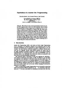
In this paper, we are interested in a special case of HTN planning, namely HTN planning with Ordered Task Decomposition (OTD). This special case was first introduced in the SHOP system [Nau et al., 1999; 2000]. The difference between SHOP and most other HTN-planning algorithms is that SHOP plans for tasks in the same order that they will later be executed. Planning for tasks in the order that those tasks will be performed makes it possible to know the current state of the world at each step in the planning process, which reduces the complexity of reasoning by eliminating a great deal of uncertainty about the world. This makes it easy to incorporate substantial inferencing and reasoning power into the planning system, including the ability to call external programs and the ability to perform numeric computations. In order to do planning in a given planning domain, SHOP needs to be given knowledge about that domain. SHOP’s knowledge base contains operators and methods. Each operator is a description of what needs to be done to accomplish some primitive task, and each method is a prescription for how to decompose some compound (abstract) task into a totally ordered sequence of subtasks, along with various restrictions that must be satisfied in order for the method to be applicable. More than one method may be applicable to the same task, in which case there will be more than one possible way to decompose that task. Given the next task to accomplish, the SHOP algorithm nondeterministically chooses an applicable method, instantiates it to decompose the task into subtasks, and then chooses and instantiates other methods to decompose the subtasks even further. The deterministic implementation of the SHOP algorithm uses depth-first backtracking: if the constraints on the subtasks prevent the plan from being feasible, then the implementation will backtrack and try other methods. As an example, Figure 1 shows two methods for the task of travelling from one location to another: travelling by air, and travelling by taxi. Travelling by air involves the subtasks of purchasing a plane ticket, travelling to the local airport, flying to an airport close to our destination, and travelling from there to our destination. Travelling by taxi involves the subtasks of calling a taxi, riding in it to the final destination, and paying the driver.


Task

travel by air long travel-distance

buy ticket(ax, ay)

travel(x, ax)

7

travel(x,y)

travel(UMD, MIT) buy ticket(BWI, Logan) travel by taxi travel(UMD, BWI) Methods get taxi ride taxi(UMD, BWI) Preconshort travel-distance pay driver ditions fly(BWI, Logan) travel(Logan, MIT) get-taxi ride-taxi (x,y) pay-driver get taxi ride taxi(Logan, MIT) fly(ax, ay) travel(ay, y) pay driver Subtasks

Figure 1. Travel planning example. Note that each method’s preconditions are not used to create subgoals (as would be done in ). Rather, they are used to determine whether or not the method is applicable: thus in Figure 1, the travel by air method is only applicable for long distances, and the travel by taxi method is only applicable for short distances. Now, consider the task of travelling from the University of Maryland to MIT. Since this is a long distance, the travel by taxi method is not applicable, so we must choose the travel by air method. As shown in Figure 1, this decomposes the task into the following subtasks: (1) purchase a ticket from Baltimore-Washington International (BWI) airport to Logan airport, (2) travel from the University of Maryland to BWI, (3) fly from BWI airport to Logan airport, and (4) travel from Logan airport to MIT. For the subtasks of travelling from the University of Maryland to BWI and travelling from Logan to MIT, we can use the travel by taxi method to produce additional subtasks as shown in Figure 1. Here are some of the complications that can arise during the planning process: • The planner may need to recognise and resolve interactions among the

subtasks. For example, in planning how to travel to the airport, one needs to make sure one will arrive at the airport in time to catch the plane. To make the example in Figure 1 more realistic, such information would need to be specified as part of SHOP’s methods and operators. • In the example in Figure 1, it was always obvious which method to use. But in general, more than one method may be applicable to a task. If it is not possible to solve the subtasks produced by one method, SHOP will backtrack and try another method instead. 3.2 HTN-planning with OTD: Syntax and Semantics We use the same definitions for variable and constant symbols, predicate symbols, and terms, as in the SHOP planning system [Nau et al., 1999;

8


2000]. Our definitions for logical atoms, states, tasks, task networks, axioms, operators, and methods are adapted from SHOP. Following the notation used in SHOP, we will write logical atoms using the format (name t1 t2 . . . tn ), where name is a predicate symbol, and t1 , t2 , . . . , tn are terms. In SHOP we can classify the atoms into three kinds: • Rigid Atoms: These are atoms whose truth values never change during

planning. These atoms appear in states, but do not appear in the effects of planning operators nor in the heads of Horn clauses. • Primary Atoms: These atoms can appear in states and in the effects of planning operators, but cannot appear in the heads of Horn clauses. • Secondary Atoms: These are the ones whose truth values are inferred rather than being stated explicitly. They can appear in the heads of Horn clauses, but cannot appear in states nor in the effects of planning operators. Now, we define the states and the axioms as in SHOP: DEFINITION 1 (States (S), Axioms (AX )). A state S is a set of ground primary atoms. An axiom is an expression of the form a ← l1 , . . . , ln , where a is a secondary atom and the l1 , . . . , ln are literals that constitute either primary or secondary atoms. Axioms need not be ground. We assume that the set of axioms does not contain cycles through negation.1 SHOP starts with a state S and modifies this state by taking into account the delete and add lists of the operators in the plan. Axioms are used only to check whether the preconditions of methods are satisfied. A precondition might not be explicitly satisfied (in the sense that the atom in question is contained in S), but might be caused by S and the axioms AX . The precise definition of this relation “caused by” is given as follows and extended in Subsection 4. DEFINITION 2 (Literal caused by (S,AX )). A literal l is caused by (S, AX ) if l is true in all answer sets of S ∪ AX . Because of our assumption on AX , the set of axioms constitutes a stratified logic program which has exactly one answer set. This ensures that any 1 This is just to ensure that a unique stable model always exist and thus the state is always complete (see the next definition). Without this condition, our approach is still complete but no more correct wrt. SHOP: SHOP does not terminate while our translation still gets meaningful results.


9

state described by the stable model of S ∪ AX is complete: any literal is either caused or its negation is caused. In order to check which literals follow from (S, AX ), SHOP uses an axiomatic inference procedure. To discuss this procedure, we need to make a distinction between the abstract SHOP algorithm and the SHOP implementation. On one hand, the abstract SHOP algorithm is nondeterministic and it makes no commitment to what inference procedure is used for checking whether literals follow from (S, AX ). The completeness proof for SHOP [Nau et al., 2000] says that if the inference procedure is complete, then SHOP is complete (i.e., if a planning problem has a solution, then at least one of SHOP’s execution traces will find a solution). On the other hand, the SHOP implementation uses an inference procedure that does a depth-first search similar to the one in Prolog. This inference procedure is complete only if the axioms satisfy some restrictions similar to those needed in Prolog (no positive cycles, no cycles through negation).2 However, all the axioms AX we are dealing with in this paper are of this sort. In fact, checking causality for these simple instances can be done in linear time. A task is an expression of the form (name t1 t2 . . . tn ), where name (the task’s name) is a task symbol, and t1 , t2 , . . . , tn (the task’s arguments) are terms. A ground task is a task that has no variables in its arguments. A task can be either primitive (if it is to be accomplished directly in the world) or compound (if it is to be decomposed into other tasks). We use a prefix ? to denote a variable (such as ?x and ?y) and ! to denote the name of a primitive task. For example, to tell the planner that getting a taxi, riding in it, and paying the driver are primitive tasks, we would give them names like !get-taxi, !ride-taxi, and !pay-driver. Tasks using these names are (!get-taxi ?x), (!ride-taxi ?x ?y), or (!pay-driver ?x ?y). A task list is a list of tasks, like the following: ((!get-taxi ?x) (!ride-taxi ?x ?y) (!pay-driver ?x ?y))) A ground task list is a task list that consists of only ground tasks, like the following: ((!get-taxi umd) (!ride-taxi umd mit) (!pay-driver umd mit))) An operator specifies how to accomplish a primitive task by modifying the current state of the world by removing every atom in its delete list and by adding every atom in its add list. 2 In addition, the SHOP implementation also computes its task decompositions using a depth-first search. Thus, in order to achieve completeness, the HTN methods also need to satisfy a similar acyclicity restriction.

10


DEFINITION 3 (Operator: (Op h ²del ²add ) ). An operator is an expression of the form (Op h ²del ²add ), where h (the head ) is a primitive task and ²add and ²del are lists of primary atoms (called the add- and delete-lists, respectively). The set of variables in the atoms in ²add and ²del must be a subset of the set of variables in h.3 As an example, here is a possible implementation of the get-taxi operator from Figure 1: (:Op (!get-taxi ?x) ((taxi-called-to ?x)) ((taxi-standing-at ?x))) Operators are used in decomposition of primitive tasks during planning: DEFINITION 4 (Decomposition of Primitive Tasks). Let t be a primitive task, and let Op = (Op h ²del ²add ) be an operator. Suppose that θ is a unifier for h and t. Then the ground operator instance (Op)θ is applicable to t, in which case we define the decomposition of t by Op to be (Op)θ. The decomposition of a primitive task by an operator results in a ground instance of that operator – i.e., it results in an action that can be applied in a state of world. We now define the result of such an application: DEFINITION 5 (Plans, result(S,π)). A plan is a list of heads of ground operator instances.4 A plan π is called a simple plan if it consists of the head of just one ground operator instance. Given a simple plan π = (h), we define result(S, π) to be the set S \ ²del ∪ ²add obtained by deleting from S all atoms in ²del and by adding all ground instances of atoms in ²add . If π = (h1 , h2 , . . . , hn ) is a plan and S is a state, then the result of applying π to S is the state result(S, π) = result(result(. . . (result (S, h1 ), h2 ), . . .), hn ). In SHOP, a method specifies a possible way to accomplish a compound task. The set of methods relevant for a particular compound task can be seen as a recursive definition of that task. 3 Unlike

the operators used in , ours have no preconditions. Preconditions are not needed for operators in our formulation, because they occur in the methods that invoke the operators. 4 In Definition 8, we will require that in any planning domain, every planning operator must have a unique name. This is sufficient to guarantee that every plan specifies an unambiguous sequence of operator instances.


11

DEFINITION 6 (Method: (Meth h ρ t) ). A method is an expression of the form (Meth h ρ t) where h (the method’s head ) is a compound task, ρ (the method’s preconditions) is a conjunction of literals and t is a totally-ordered list of subtasks, called the decomposition list of the method. The set of variables that appear in the decomposition list of a method must be a subset of the variables in h (the head of the method) and ρ (the preconditions of the method). 5 Here is a possible implementation of the travel-by-taxi method from the same figure: (:Meth (travel ?x ?y) ((smaller-distance ?x ?y)) ((!get-taxi ?x) (!ride-taxi ?x ?y) (!pay-driver ?x ?y))) Let m = (Meth h ρ t) be a method. Note that there may be variables in ρ that do not appear in the head h of the method m. These variables are called the unbound variables of m. During planning, these variables are grounded when the method is used for the decomposition of a compound task, as described below. DEFINITION 7 (Decomposition of Compound Tasks). Let t be a compound task, S be the current state, Meth = (Meth h ρ t) be a method, and AX be an axiom set. Suppose that θ is a unifier for h and t, and that θ0 is a unifier such that all literals in (ρ)θθ0 are caused wrt. S and AX (see Definition 2). Then, the ground method instance (Meth)θθ0 is applicable to t in S, and the result of applying it to t is the ground task list r = (t)θθ0 . The task list r is the decomposition of t by Meth in S. Note that the decomposition of a compound task by a method does not change the state of the world. The result of such a decomposition is a ground task list that needs to be further decomposed until we get a list of only ground operator instances — i.e., a plan. DEFINITION 8 (Planning Domain Descriptions and Problems). A planning domain description D is a triple consisting of (1) a set of axioms, (2) a set of operators such that no two operators have the same head, and (3) a set of methods. 5 This restriction is needed to ensure that our programs do not violate the safeness restrictions of the ASP systems we are using. However, the restriction has no effect on the expressivity of our formalism. Any method that does not satisfy the restriction can easily be translated into an equivalent method that does satisfy the restriction, by introducing a dummy precondition that can always be satisfied.

12


A planning problem is a triple (S, t, D), where S is a state, t= (t1 , t2 , . . . , tk ) is a ground task list, and D is a planning domain description. We now define a solution of a planning problem. DEFINITION 9 (Solutions). Let P = (S, t, D) be a planning problem and π = (h1 , h2 , . . . , hn ) be a plan. Then, π is a solution for P ,6 if any of the following is true: • Case 1: t and π are both empty, (i.e., k = 0 and n = 0); • Case 2: t = (t1 , t2 , . . . , tk ), t1 is a ground primitive task, (h1 ) is the

decomposition of t1 , and (h2 . . . hn ) solves (result(S, (h1 )), (t2 , . . . , tk ), D); • Case 3: t = (t1 , t2 , . . . , tk ), t1 is a ground compound task, and

there is a decomposition (r1 . . . rj ) of t1 in S such that π solves (S, (r1 , . . . , rj , t2 , . . . , tk ), D). The planning problem (S, t, D) is solvable if there is a plan that solves it. One important issue that we want to point out about this definition is that the SHOP formalism does not require the tasks to be ground. This and the restriction in Definition 6, are both necessary in the formalism of our translation method, simply because, otherwise, the logic programs that are generated by our translation would contain rules that violate the safeness conditions that are imposed by current ASP systems. However, this is a mild restriction and can always be ensured by adding dummy predicates. It will be very helpful for the main proof of Theorem 30 to introduce the notion of a search ree. The successful paths of this tree correspond to the solutions of the planning problem. DEFINITION 10 (Search Tree for Trans(·)). Given a planning problem (S, t, D), we define the search tree for (S, t, D) as follows. Nodes of the tree are triples of the form hS 0 , tcaused , t0 i, where S 0 is a state, tcaused is an ordered list of ground primitive tasks, and t0 is a (possibly empty) ordered list of ground (compound or primitive) tasks. The start node consists of the triple hS, ∅, ti. Leaf nodes are those of the form hS, tcaused , ∅i. Branches ending in such leaves are called successful. Given a node hS 0 , tcaused , t0 i with t0 6= ∅, its children are defined as follows: • If the first task in t0 is primitive and there is an operator in D for it, then

there is exactly one child hS ? , t?caused , t? i. t?caused is the old list tcaused plus this first task appended. S ? is obtained by modifying S 0 according to the add and delete lists of the operator. t? is t0 with the first element 6 Or equivalently, we say that π solves P , or π achieves t from S in D (we will omit the phrase “in D” if the identity of D is obvious).


13

m1(t1)

m3(t1)

m1(t111)

m2(t1)

m2(t111)

…

o(t1111)

…

o(t121)

…

m1(t122)

… … …

… …

FAILURE!

…

o(ti)

…

SUCCESS!

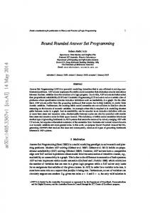
Figure 2. Search Tree for (S, t, D). Edge labellings mi (t) (resp. o(t)) represent a method (resp. an operator) application to a task t, which is compound (resp. primitive). deleted. The edge to this child is labelled with the name of this first task. If the first task in t0 is primitive and there is no operator, then there is no child and the branch is marked with Failure. • If the first task in t0 is compound, and there exist method instances applicable to it (according to Definition 7), then each such method instance mi leads to a child node hS, tcaused , ti i the edge to which is labelled with mi . ti is obtained from t0 by replacing the first task by the subtasks according to mi . If the first task in t0 is compound, and there are no methods applicable to it, then the branch is marked Failure. We define the task-depth of a node and its edges as follows. The start node gets task-depth 0. Whenever a method is used to extend a node, the children nodes keep the same task-depth. When an operator is applied, and thus a task is moved from t0 into tcaused then the task depth of the child node is incremented by one. Obviously, the task depth of a node is the size of the list of tasks in tcaused . Such a tree (or a part thereof) is depicted in Figure 2. Note that there can be different paths (corresponding to the application of different methods) that finally lead to the same plans (as a list of the heads of ground instances

14


of operators). DEFINITION 11 (Solution Set of a Planning Problem: Sol(S, t, D)). Let P = (S, t, D) be a planning problem, and suppose T is the search tree for P . Then, Sol(S, t, D) is a multi set: it contains exactly the ordered lists tcaused in the leaf nodes that are reached by the successful paths of T . We also say T represents Sol(S, t, D). Note that Sol(S, t, D) may contain more than one copy of the same plan.

4

Encoding HTN planning in Nonmonotonic Logic Programming

Our approach of encoding HTN planning problems as logic programs is based on SHOP’s representation of a planning problem as described in the last section. We now present the first steps of a causal theory of HTN planning based on that formalism. This theory serves as an intermediate step and a motivation for our translation methodology, which is given in the next subsection. We conclude this section with the formalisation of a particular example. 4.1 Causal Theory for HTN Planning In this section we prepare the ground for our translation in the next subsection. We give some definitions of a causal theory for HTN planning in a SHOP-like ordered task decomposition. DEFINITION 12 (Causable Literals). Let S be a state, and let D be a planning domain description. A literal l is causable wrt. (S,D) if it is caused by (S, AX ) (according to Definition 2), where AX is the set of axioms in D. A conjunction of literals is causable wrt. (S, D) if every literal in the conjunct is causable wrt. (S, D) (according to the Definition 2). DEFINITION 13 (Causable Tasks). Let S be a state, and let D be a planning domian description. The definition of an ordered list of ground tasks to be causable wrt. (S, D) comes in three steps. 1. The empty list [ ] is causable wrt. (S, D). 2. An ordered list of ground primitive tasks t1 , . . . , tn is causable wrt. (S, D) if for each ti , there exists an operator (Op h ²del ²add ) ∈ D and there is a unifier θ such that ti = (h)θ. 3. An ordered list of ground tasks t1 , . . . , tj , . . . , tn , where tj is a ground compound task and all tasks t1 , . . . , tj−1 are ground primitive tasks, is causable wrt. (S, D) if the following holds:


15

• There exists a method (Meth h ρ {tj1 , . . . , tjm }) ∈ D for tj , and there is a unifier θ such that tj = (h)θ; and • There exists a unifier θ0 such that the preconditions list (ρ)θθ0 is causable wrt. (result(S, (t1 , . . . tj−1 )), D); and • The ordered decomposition list (t1 , . . . , tj−1 , (tj1 )θθ0 , . . . , (tjm )θθ0 , tj+1 , . . . tn ) is causable wrt. (S, D). Note that this is a recursive definition. The condition in the last part (compound tasks) eventually ends when there are only primitive tasks left, and thus the second part (primitive tasks) can be applied. The notion of literals being causable is used to make sure that the appropriate methods (used to decompose the task tj ) can be applied in the current state. Using this causal theory as an intermediate step, we developed a systematic translation method for mapping planning problems to logic programs with negation which we illustrate in the subsequent section. The next theorem states the equivalence of the original SHOP planning framework as presented in the last section with the notion of causable tasks just introduced. THEOREM 14. Let P = (S, t, D) be a planning problem. Then, there is a solution to P if and only if the task list t is causable wrt. (S, D). Proof. Rather than giving a full proof using structural induction, we give a detailed proof sketch from which the full proof can be easily worked out. The proof starts by recursively constructing the solution of an HTN planning problem (S, t, D) and showing the causal relationships based on our causal theory at the same time. Suppose there exists a solution to (S, t, D). If t is empty, then (S, t, D) contains exactly one plan, namely the empty plan. This is because of the fact that there will be no tasks to be accomplished—thus, no task to be causable . If t is not empty, and consists of primitive tasks only, then there must be operators for all these tasks and thus, by Definition 13 (2nd step), t is causable wrt. (S, D). We now reduce the general case to the case where only primitive tasks occur. Let t be non-empty, and assume it contains compound tasks. Then we recursively carry out the task decompositions (see Definition 7) until we reach a list of ground primitive tasks. This is possible because a solution exists (this solution is given by the final list of primitive tasks). Note that

16


there might exist different such lists, corresponding to different choices of decompositions via methods. But this list is causable according to the second part of Definition 13 (primitive tasks). Now, according to the third part of Definition 13, we can recursively replace the primitive tasks with the compound tasks they were induced from (via methods) and we get the result that all the intermediate ordered lists obtained in that way themselves are causable wrt. (S, D). Note that the conditions in the third part of Definition 13 correspond exactly to the notion of the decomposition of a compound task (Definition 7). Therefore, it follows from the recursive construction above that if a list of ground tasks t is achieved according to our planning theory, it must be causable as well. The proof of the converse is similar. Once a list of ground tasks t is causable wrt. (S, D), we can find a list of primitive tasks that is causable. This list is obtained by certain decompositions, and these decompositions constitute a solution of the planning problem. ¥ 4.2

Encoding Planning Problems as Logic Programs

In this section, we present our translation method for encoding planning problems as logic programs with ASP semantics. Our translation method is a general technique that is independent from the implementation details and syntactic requirements of the any underlying ASP system. Note that there are several differences between the syntactic requirements of the ASP systems. In this respect, the presentation in this section is given in a more conceptual level in general; however, where necessary, we adapted the syntax of Smodels.7 Translating a planning problem (S, t, D) to its logic program counterpart requires encoding the initial state and the state transition characteristics of SHOP, the goal tasks and the ordered task decomposition technique in SHOP, and the domain description including the axioms, the operators, and the methods, which are given in the description of a planning problem. For this reason, we describe our translation method in several steps such that each step encodes a part of the complete translation corresponding to the components of a planning problem as described above. Combining these steps yield a complete logic program in ASP semantics that is capable of 7 However, note that when implementing our translation methodology, one must address the syntax requirements of the underlying system that is being used. In this paper, we concentrated on the two ASP systems Smodels and DLV , so we made system-specific syntactic changes to the conceptual description of our translation method during the implementation in these systems. Our complete implementation of planning examples for both DLV and Smodels are available at .


17

solving planning problems in the way that SHOP does. We now present our main definition: DEFINITION 15 (Trans((S, t, D)): Translation for the Planning Problem). Let P = (S, t, D) be a planning problem. The logic program Trans((S, t, D)) that solves P is defined as Trans((S, t, D)) = Trans(⊥) ∪ Trans(S) ∪ Trans(t) ∪ Trans(AX ) ∪ Trans(OP) ∪ Trans(F) ∪ Trans(MET H), where • Trans(⊥) is the logic program segment that marks the successful termi• • • • • •

nation of the planning process, Trans(S) is the logic program segment that encodes the initial state S, Trans(t) is the logic program segment that encodes the goal task list t, Trans(AX ) is the logic program segment that encodes the axioms given in the domain description D, Trans(OP) is the logic program segment that encodes the operator descriptions given in D, and Trans(F) is the logic program segment that encodes the state-transition characteristics of SHOP, and Trans(MET H) is the logic program segment that encodes the method descriptions given in D.

In the following subsections, we give the definitions for the logic program segments mentioned above. The Time Line In order to be able to keep track of different states of the world in an answer set of a logic program, we attached a time variable that will occur in many predicates in our translation. The domain of a time variable is a time line, which is a set of integers {0, 1, . . . , τ }, where τ is called the end point of the time line. Given a planning problem P = (S, t, D), we need to know τ in advance in order for our translation methodology to work. P does not specify this information since SHOP does not need a notion of time line during planning — the search process naturally differentiates different states of the world. One way to determine a correct value for τ is an incremental approach. That is, we start with τ = 0, use our translation to produce the logic program Trans((S, t, D)), and generate the answer sets of Trans((S, t, D)). Then, we increment τ , and repeat the whole process until no new answer

18


sets are generated by Trans((S, t, D)). Note that, using this approach, we eventually generate all of the possible answer sets of Trans((S, t, D)), as shown in Theorem 30. An alternative approach would be as follows. Let Sol(S, t, D) be the set of solutions of P , as in Definition 11. Then, we define τ as τ = max{|π| : π ∈ Sol(S, t, D)}, where |π| denotes the size of the solution π. Note that we can find the set Sol(S, t, D) by solving P using SHOP. We use time variables in various rules in our translation, so before going into the details of the translation, we believe that the following points are worth noting: 1. As described above, we assume that planning starts at time point 0 (see Definitions 16 and 19). 2. Planning proceeds by selecting a task to be accomplished next (see Definition 19. The rules about taskT BA and causable are given in Definition 17). Note that the task to be decomposed may be either primitive or compound. 3. The time variable T is incremented only when the task to be decomposed is a primitive task and there is an operator for it (a simple reduction) in the domain description provided as a part of the planning problem (see Definition 18). This means that, in general, there may be more than one task that is selected and decomposed at a particular time point T . However, among these tasks, there is only one primitive task at any particular point in time. For example, consider Figure 2. Task t1 is a compound task and so are t111 and t1111 (obtained by respective methods). So taskT BA(t1 , 0), taskT BA(t111 , 0), taskT BA(t1111 , 0) are all true (resp. hold in a stable model). Only after the primitive task t1111 has been accomplished by an operator is the time incremented by 1. 4. As a result of this formulation, the task depth in the search tree corresponds to the value of the time variable T . Encoding the Initial State SHOP’s initial state is a set of ground atoms. In this respect, given a planning problem (S, t, D), the logic program encoding for the initial state S is defined as follows:


19

DEFINITION 16 (Trans(S): Translation for Initial State). Given a planning problem (S, t, D), for each ground atom a ∈ S, the logic program Trans(S) contains the rule

in state(a, 0) : −

where 0 indicates the initial time. Encoding the Goal Task(s) Given a planning problem (S, t, D), where S is the initial state, t is a ground task list, and D is a domain description for this planning problem, the aim of the planning process is to find a plan that accomplishes all of the (goal) tasks in t from the initial state S in the order they are given (according to Definition 8). A task is accomplished if and only if it is causable with respect to the initial state and the domain description given in the planning problem, and this is due to the Definition 13 and a direct consequence of Theorem 14. In this respect, planning proceeds by selecting a task as the “current task” – i.e., the task that the planner will try to accomplish next. In the logic programs produced by our translation, this is encoded by using a special predicate defined as follows: DEFINITION 17 (Tasks To Be Accomplished). Given a planning problem (S, t, D), we define a special predicate taskT BA n for each possible task (e.g. primitive or compound) such that if the task that needs to be decomposed at time T is h ≡ (nameh arg1 arg2 . . . argN ) then taskT BA n(nameh , arg1 , arg2 , . . . , argN , T ) denotes this fact and n is a natural number which equals N + 2 (n is the number of arguments of this predicate). As an example, if the task to be accomplished is travelling from UMD to MIT denoted as (travel umd mit), then we use the predicate taskT BA 4(travel, umd, mit, T ) to denote this fact. For the sake of clarity, we will use the shorthand notation taskT BA(h, T ) in the rest of the paper. We define the fact that whether a task is causable as follows: DEFINITION 18 (CAUSABLE).

Given a ground task t, we define

20


CAU SABLE(t, Ts , Ta ) as follows:  f alse         f alse    taskT BA(t, Ts ) and Ta = Ts + 1         causable(t, Ts , Ta )   

if t is a primitive task and there is no operator for it in D, if t is a compound task and there is no method for it in D, if t is a primitive task and there is an operator for it in D, if t is a compound task and there is a method for it in D.

where Ts denotes the time when the task t was selected to be decomposed and Ta denotes the time when t is actually accomplished (i.e., Ta is the time when t is caused). In the definition above, causable(t, Ts , Ta ) is a shorthand notation for the predicate causable n(namet , arg1 , arg2 , . . . , argN , Ts , Ta ) in which the symbol n = N +3 denotes the number of arguments of the predicate causable n. For the sake of clarity, we will use causable(t, Ts , Ta ) in the rest of the paper. We are now ready to define the logic program segment that encodes the goal task list of a given planning problem. DEFINITION 19 (Trans(t): Translation for Goal Tasks). Given a planning problem (S, t, D), let t = h1 , h2 , . . . , hn be the ordered sequence of ground tasks. Then, Trans(t) is the logic program that contains one rule for each ground task hi , where i = 1, 2, . . . , n, as follows: 1. Case 1: i = 1, taskT BA(h1 , 0) : − 2. Case 2: Otherwise, taskT BA(hi , Ti ) : −

CAU SABLE(hi−1 , Ti−1 , Ti ), Ti ≥ Ti−1 .

Note that if there exists only one goal task to be accomplished for the problem in hand, then only defining the first rule will suffice. Definition 19 enforces the fact that a goal task hi is designated as the current task to be accomplished if the previous goal task hi−1 in t is causable. This is a direct consequence of our Theorem 14. The planning process terminates successfully when all of the goal tasks are accomplished (i.e., caused) in the order they are given in the planning problem. The following definition is given to encode the successful termination of the planning process.


21

DEFINITION 20 (Trans(⊥): Successful Termination). Given a planning problem (S, t, D), the logic program segment Trans(⊥) that encodes the successful termination of the planning process (i.e., the fact that a solution to the given planning problem is found) is defined as follows: plan f ound plan f ound

:− :−

CAU SABLE(hn , Tn , Tn+1 ), Tn+1 ≥ Tn . not plan f ound.

where hn is the last goal task in t, Tn denotes the time at hn is decomposed by a simple reduction for it (see Definition 7), and Tn+1 is the time at which hn is causable (accomplished). These two rules together state that if the last goal task is causable then there is a plan (solution) for the planning problem (S, t, D) as a result of Definition 19. Otherwise, there is none. Encoding the Axioms We now define the logic program segment that encodes the axioms of a domain description. We start with notion of translation for a literal. DEFINITION 21 (Translation for Literals). Given a literal, l, we define C(l, T ), the translation of l at time T , as ½ in state(a, T ) if l = a is a positive literal, C(l, T ) := not in state(a, T ) otherwise. DEFINITION 22 (Trans(AX ): Translation for Axioms). Given a planning problem (S, t, D), Trans(AX ) is the logic program segment that contains the following rules: for all “ a ← l1 , . . . , ln ” ∈ AX , in state(a, T ) : − C(l1 , T ), C(l2 , T ), . . . , C(ln , T ), where C(li , T ) is the translation of the literal li , as defined in Definition 21 above. Encoding the Operators and the State Transitions SHOP uses the operator descriptions in D in decomposition of primitive tasks that needs to be accomplished during planning. In the translation, the logic program segment that encodes the operators in D is given as follows: DEFINITION 23 (Trans(OP): Translation for Operators). Given a planning problem (S, t, D), for all Op ∈ OP, Trans(Op) is the logic program that contains the following rules: for all a ∈ Del(Op): out state(a, T + 1) : − taskT BA(h, T ).

22


and for all a ∈ Add(Op): in state(a, T + 1) : − taskT BA(h, T ). where h is a primitive task – i.e., the ground head of the operator that is used in the decomposition of h. Note that these two rules encode the delete- and the add-lists of the operator respectively. The result of a decomposition of a primitive task by an operator application is a new state of the world, which is generated by deleting all of the atoms that are in the delete-list of that operator from the current state and by adding all of the atoms that are in the add-list of that operator to the current state. An operator only describes the change it causes to occur in the current state. The planner is still responsible for keeping track of the other facts that remain unchanged after an operator application. This is known as the famous Frame Problem in AI Planning. In the translation, the logic program segment that addresses the frame problem is defined as follows: DEFINITION 24 (Trans(F): Keeping Track of the State S). The logic program segment Trans(F) that encodes the frame axiom is defined as follows: in state(A, T + 1)

: − in state(A, T ), not out state(A, T + 1).

Note that the state of the world in SHOP consists of only positive ground primary atoms. Basically the above rule states that if a positive ground atom, a, is initially true, then it should be true in the next state unless it has been marked as to be deleted during the transition from the current state to the next state. Encoding the Methods SHOP uses the method descriptions in D in decompositions of compound tasks that need to be accomplished during planning. Before proceeding with the definition of the logic program segment that encodes the methods in D, we give the following definition: DEFINITION 25 (Methods for a Compound Task). Given a planning problem (S, t, D) and a compound task h ≡ (nameh arg1 arg2 . . . argN ), we define a special predicate method n i(nameh , arg1 , arg2 , . . . , argN , T ) for each method mi ∈ D whose head unifies with h. The symbol n in the predicate name denotes the number of arguments of the predicate, i.e. n = N +2. For purposes of clarity, we will use the following shorthand notations in the rest of this paper: Given a planning problem (S, t, D) and a compound task h, if there is only one method m whose head unifies with


23

h in D then we will use method(h, T ) to refer to m, instead of the method n 1(nameh , arg1 , arg2 , . . . , argN , T ) predicate as defined above. If there are more than one methods mi for h then we will use the notation methodi (h, T ) for each such method mi . We present the translation for methods of SHOP in four steps: (1) the translation for the nondeterministic choice of applying alternative methods to a particular compound task; (2) the translation for evaluating the preconditions of a method in order to decide whether it is applicable to a particular compound task; (3) the translation for the task decomposition specified by a method; and (4) the translation for the accomplishment of a particular task by a method. Given a SHOP method, if the translations in these four steps are performed, then we produce a logic program segment, Trans(MET H), which is the ASP encoding of that method. DEFINITION 26 (Translation for Encoding Alternative Methods). Given a planning problem P = (S, t, D), let h be a compound task that needs to be accomplished in the solution of P . Suppose D contains N methods whose heads unify with h; namely, m1 , m2 , . . . , mN . Then, the logic program segment that encodes the nondeterministic choice of which method to apply to the task h is as follows: for i, j = 1, . . . , N , V methodi (h, T ) : − i6=j not methodj (h, T ), taskT BA(h, T ). Intuitively, the rules in Definition 26 enforce the translation to create N different answer sets for N possible method applications to the task h. This is due to the fact that each such method specifies a different way to decompose the task h, and therefore, the planner can find different solutions due to each such method. Next, we present the translation for evaluating the preconditions of each such method. Note that if the precondition of the method is not satisfied in the state of the world, then the method cannot be applied to the task h. DEFINITION 27 (Translation for Precondition Evaluations). Let h be a compound task that needs to be accomplished, mi be a method whose head unifies with h, and ρ be the preconditions of mi . Then, we have two steps: 1. Let p ∈ ρ be a precondition of m and χ1 , χ2 , . . . , χf be the unbound variables in p such that if f = 0 then p has no such variables. Suppose that Rj denotes the range of χj in p – i.e., Rj is the set of all possible instantiations of χj in the world. Then, for each unbound variable χj of p, we create new variable symbols χj,k such that j = 1, . . . , f and k = 1, . . . , |Rj |.

24


2. For each precondition p ∈ ρ, • if p does not contain unbound variables, then we have

checked state(p, T ) : − C(p, T ), methodi (h, T ). where C(p, T ) is as defined in Definition 21. • Otherwise, we have checked state(p(χ1,1 , χ2,1 , . . . , χf,1 ), T ) : − methodi (h, T ), in state(p(χ1,1 , χ2,1 , . . . , χf,1 ), T ), not checked state(p(χ1,1 , χ2,1 , . . . , χf,2 ), T ), .. . not checked state(p(χ1,1 , χ2,1 , . . . , χf,|Rf | ), T ), .. . not checked state(p(χ1,1 , χ2,|R2 | , . . . , χf,|Rf | ), T ), not checked state(p(χ1,2 , χ2,1 , . . . , χf,1 ), T ), .. . not checked state(p(χ1,|R1 | , χ2,|R2 | , . . . , χf,|Rf | ), T ), Vf j=1 χj,1 ! = χj,2 ! = . . . ! = χj,|Rj | . where χ1 , χ2 , . . . , χf are the unbound variables in p. Intuitively, the rules of Definition 27 create an answer set for each possible instantiation of the unbound variables of mi in the world. This is due to the fact that SHOP creates an instance of mi for each instantiation of the unbound variables in mi , and decomposes the task h with each such method instance. In order for our translation to be correct, we need to simulate this behavior of SHOP in our translation since ASP systems do not provide such semantics, to the best of our knowledge. Note that for each precondition p ∈ ρ, there must be at least one answer set in which both methodi (h, T ) and checked state(p, T ) are true for the method mi to be applicable to the task h in the current state of the world (denoted by the time variable T ). If there is no such answer set then it means that mi is not applicable to h. Now that we have established the rules for checking the applicability of mi to h, we are ready to give the definition for the decomposition of the task h by mi . DEFINITION 28 (Translation for Method Decomposition). Let h be a compound task that needs to be accomplished, and let mi be a method


25

that is applicable to h. Then, the decomposition of h by mi is encoded by the following rules: taskT BA(t1 , T )

:−

taskT BA(t2 , T2 )

:−

.. . taskT BA(tn , Tn )

.. . :−

method i (h, T ), V checked state(p, χ1 , χ2 , . . . , χf , T ). p∈ρ method (h, T ), i V p∈ρ checked state(p, χ1 , χ2 , . . . , χf , T ), CAU SABLE(t1 , T, T2 ), T2 ≥ T. .. . method i (h, T ), V checked state(p, χ1 , χ2 , . . . , χf , T ), p∈ρ CAU SABLE(tn−1 , Tn−1 , Tn ), Tn ≥ Tn−1 .

where χ1 , . . . , χf are the unbound variables of the precondition p, and t1 , . . . , tn are the subtasks of m –i.e., the ordered list of tasks in the decomposition list of m. The translation in Definition 28 encodes the fact that the decomposition of each subtask tk can only be done if the previous subtask tk−1 has been already accomplished – i.e. tk−1 has been already CAU SABLE. The only exception is the first task, which is decomposed if and only if the particular method, h, has been chosen to be applied to the current task in the planning process. This property is encoded by using the CAU SABLE(tk , Tk , Tk+1 ) construct for each subtask tk (see Definition 18). The time point Tk denotes the time when the current task is decomposed and Tk+1 denotes the time when it is accomplished – i.e. causable. By this way, we can identify the exact place where a specific task is causable in the entire search tree. Finally, we have the definition of the accomplishment of a task by a particular method. DEFINITION 29 (Translation for Accomplishment of Compound Tasks). Let h be a compound task that needs to be accomplished, let mi be a method that is applicable to h, and suppose that h has been already decomposed into its subtasks tk specified by the decomposition list of mi . Then, the accomplishment (i.e., causation) of h by the method mi is encoded as follows: causable(h, T, Tn+1 )

:− V methodi (h, T ), p∈ρ checked state(p, χ1 , χ2 , . . . , χf , T ), CAU SABLE(tn , Tn , Tn+1 ), Tn+1 ≥ Tn .

where χ1 , . . . , χf are the unbound variables of the precondition p of m.

26


Intuitively, h is accomplished (i.e., caused) when/if the last subtask in its decomposition by mi is accomplished (i.e., caused.) This is a direct consequence of Theorem 14. Note that some of the rules given Definitions 26 and 27 could also be encoded into disjunctive rules, which seems to be conceptually simpler. However, not all ASP systems do handle disjunctions. Therefore, we decided to use non-disjunctive rules. At this point, we refer to the discussion in subsection 5.2. 4.3

A Translation Example: An Elevator Domain

One of the planning domains in the AIPS-2000 planning competition was the Miconic-10 Elevator domain. In order to accommodate the representational power of different planning systems, several different versions of this domain were used in the competition. The simplest version, which we will call Miconic-10-simtest,8 has the following specifications: (1) the planner simply has to generate plans to serve a group of passengers of whom the origin and destination floors are given, and (2) there are no constraints such as satisfying space requirements of passengers or achieving optimal elevator controls. Below, we describe how to use the techniques in the previous section to translate an HTN version of the domain into an ASP encoding. For the sake of simplicity and clarity, we present our translation methodology on a simplified and modified version of this problem domain in Smodels syntax. The SHOP axioms, operators, and methods for this problem domain are shown in Figures 3, 4, and 5, respectively. Our complete encodings of the original Miconic-10-simtest domain for both DLV and Smodels are available at . In our modified elevator example, there is only one person to be transported in a five floor building. The elevator starts its operation at the ground floor. Our passenger is at the top floor and wants to go down to the ground floor. The elevator can move between any two floors in one step; however, this movement can be either slow or fast, depending on the distance between those floors. The fast movement of the elevator depends on the amount of energy available to it. The elevator has initially enough energy for such movements. However, a fast movement decreases the total energy of the elevator by a specific amount. More specifically, a fast movement between two adjacent floors consumes one unit of energy. Unlike fast movements, slow movements do not require energy. The elevator always makes slow movements when it is empty, in order to conserve energy. 8 We use this name because the domain is available at .


27

Now, we will describe the basics of the translation process step by step as described in the previous section. Prelude We have to formulate all of the possible atoms that can ever be used during the planning process. Due to the fact that each variable in Smodels semantics must have a range of values, we must also define type predicates in our translation as described in the previous section. In a SHOP domain description, we do not need to make these definitions about the set of all possible atoms and tasks, nor about the type predicates. In our elevator example, we have the following rules for specifying the possible atoms: atom(boarded(P )) atom(goal(P )) atom(lif t at(F )) atom(destination(P, F )) atom(on f loor(P, F )) atom(on lif t(P )) atom(total energy(E))

:− :− :− :− :− :− :−

person(P ). person(P ). f loor(F ). person(P ), f loor(F ). person(P ), f loor(F ). person(P ). energy levels(E).

And also the following rules for the type predicates such as: time(0..10) :− person(p0) :− f loor(0..4) :− energy levels(0..10) : − Note that we define the time line of our logic program to be the set {0, 1, . . . , 10}. This definition is just for illustrative purposes in this example. Normally, we use one of the two techniques for defining the time lines, as described in the previous section. Encoding the Initial State The logic program segment Trans(S) consists of the following rules to specify the initial state in our encoding of the elevator example: in in in in in

state(lif t at(0), 0) state(goal(p0), 0) state(on f loor(p0, 4), 0) state(destination(p0, 0), 0) state(total energy(10), 0)

:− :− :− :− :−

As it can be seen from these rules, they specify certain ground atoms to be in the initial state of the planner (Definition 16 in the previous section).

28


;; SHOP Axioms for the simplified Miconic-10-simtest Domain. (:- (can-move-fast ?floor1 ?floor2) ((> ?floor1 ?floor2)(total energy ?energy) (≥ (- ?floor1 ?floor2) ?energy)) (:- (can-move-fast ?floor1 ?floor2) ((≤ ?floor1 ?floor2)(total energy ?energy) (≥ (- ?floor2 ?floor1) ?energy))) (:- (floorDiff ?floor1 ?floor2 ?d) ((> ?floor1 ?floor2)(assign ?d (- ?floor1 ?floor2))) (:- (floorDiff ?floor1 ?floor2 ?d) ((≤ ?floor1 ?floor2)(assign ?d (- ?floor2 ?floor1))))

Figure 3. Examples of the SHOP axioms for the simplified version of Miconic-10-simtest planning domain.

The last argument for each in state(A, T ) predicate is the time T at which the atom A holds. As mentioned before, we define the starting time of the planning process to be 0. The frame axiom Trans(F) is as follows: in state(A, T + 1)

:−

time(T ), atom(A), in state(A, T ), not out state(A, T + 1).

Encoding the Goal Task(s). Suppose we have a single goal task to accomplish, namely the task of transporting our passenger. Then, the logic program segment Trans(t) will encode this task via the following rule: taskT BA(transport person, p0, 0) : − This rule specifies that our goal task to be accomplished at the beginning of planning process is the task (transport person p0) — i.e., the task of transporting the person p0. Encoding the Axioms Suppose that we have the axioms shown in Figure 3. The intended meaning of these axioms is to decide whether the elevator can make a fast movement between the specified two floors. The criteria for this decision is that if the distance between the two floors is greater than or equal to the total energy of the elevator, then it can move fast between these two floors. The encoding


29

;; SHOP Operators for the simplified Miconic-10-simtest Domain. (:operator (!markServed ?person) ((goal ?person)) ()) (:operator (!moveSlow ?floor1 ?floor2) ((lift at ?floor1)) ((lift at ?floor2))) (:operator (!moveFast ?floor1 ?floor2 ?old ?new) ((lift at ?floor1)(total energy ?old)) ((lift at ?floor2)(total energy ?new)) (:operator (!board ?person ?floor) ((on ?person ?floor)) ((on lift ?person))) (:operator (!debark ?person ?floor) ((on lift ?person)) ((on ?person ?floor)))

Figure 4. Examples of the SHOP operators for the simplified version of Miconic-10-simtest planning domain. of this axiom as the logic program segment Trans(AX ) is straightforward: in state(can move fast(F 1, F 2), T )

: − time(T ), f loor(F 1), f loor(F 2), energy level(E), in state(total energy(E), T ), F 1 > F 2, F 1 − F 2 ≥ E. in state(can move fast(F 1, F 2), T ) : − time(T ), f loor(F 1), f loor(F 2), energy level(E), in state(total energy(E), T ), F 1 ≤ F 2, F 2 − F 1 ≥ E. in state(floorDiff(F 1, F 2, F 1 − F 2), T ) : − time(T ), f loor(F 1), f loor(F 2), F 1 > F 2. in state(floorDiff(F 1, F 2, F 2 − F 1), T ) : − time(T ), f loor(F 1), f loor(F 2), F 1 ≤ F 2.

Encoding the Operators Suppose that in the domain description of our elevator example, we have the planning operators shown in Figure 4. The first operator in Figure 4 is for the primitive task of marking a person served. This operator basically removes the (goal ?person) atom from the state of the world, which means that the goal of transporting the person ?person has been achieved. Note that this operator does not add any atoms to the state of the world. The second operator is for the primitive task of

30


moving the elevator slowly from one floor to another. It simply deletes the (lif t at ?f loor1) atom from the state, which describes the location of the elevator before it started its move, and adds the atom (lif t at ?f loor2), which describes the location of the elevator after it completed its move. The third operator is for the primitive task of moving the elevator fast. Note that this operator also changes the total amount of energy that the elevator has. The fourth and the fifth operators are for boarding a person to the elevator and for debarking a person from the elevator, respectively. In our translation, the markServed operator is encoded by a single rule: out state(goal(P ), T + 1)

:−

time(T ), person(P ), taskT BA 3(markServed, P, T ).

The encoding of the moveSlow operator corresponds the following: out state(lif t at(F 1), T + 1)

:−

in state(lif t at(F 2), T + 1)

:−

time(T ), f loor(F 1), f loor(F 2), taskT BA 4(moveSlow, F 1, F 2, T ). time(T ), f loor(F 1), f loor(F 2), taskT BA 4(moveSlow, F 1, F 2, T ).

The moveFast, board, and debark operators are encoded similarly. Encoding the Methods We have the following four methods in our domain description: We have two methods for fast transporting the person from his/her original floor to his/her destination floor. The first method is for the case in which the elevator and the person are on the same floor, so the person can be immediately boarded to the elevator and transported to his/her destination. The second method is for the case in which the elevator and the person are not on the same floor; the elevator must be first moved to the floor of the person so that the person can be transported. Figure 5 shows the SHOP specification of these two methods. We have also two methods for slow transportation of the person, similar to the ones described above. The two groups of methods – i.e., the first two and the second two – correspond to a branching (i.e, backtracking choice) point in the planner’s search space, in which different branches may possibly lead to different solution plans. However, the first two methods cannot both yield to a solution due to the way their preconditions are defined. The same is true for the second two as well. According to Definition 26, the translation of the nondeterministic choice among these four methods is the following set of rules, which correspond to the same branching point in the search space. Here, we only give the rule(s)


31

;; SHOP Methods for the simplified Miconic-10-simtest Domain. ;; Method for FAST transporting a person when the lift is at the same floor ;; as him/her. (:method (transport person ?person) ;; preconditions ((lift at ?floor1)(on ?person ?floor1)(destination ?person ?floor2) (total energy ?old)(can move fast ?floor1 ?floor2) (floorDiff ?floor1 ?floor2 ?d)(assign ?new (- ?old ?d))) ;; decomposition task list ((!board ?person ?floor1) (!moveFast ?floor1 ?floor2 ?old ?new) (!debark ?person ?floor2) (!markServed ?person))) ;; Method for FAST transporting a person when the lift is not at the same floor ;; as the person. (:method (transport person ?person) ;; preconditions ((lift at ?floorX)(on ?person ?floor1)(destination ?person ?floor2) (total energy ?old)(can move fast ?floor1 ?floor2) (floorDiff ?floor1 ?floor2 ?d)(assign ?new (- ?old ?d))) ;; decomposition task list ((!moveSlow ?floorX ?floor1)(!board ?person ?floor1) (!moveFast ?floor1 ?floor2 ?old ?new)(!debark ?person ?floor2) (!markServed ?person)))

Figure 5. Examples of the SHOP methods for the simplified version of Miconic-10-simtest planning domain. for the first method; the others are almost identical. method 3 1(transport person, P, T ) : − time(T ), person(P ), taskT BA 3(transport person, P, T ), not method 3 2(transport person, P, T ), not method 3 3(transport person, P, T ), not method 3 4(transport person, P, T ). We now describe the encoding for evaluting the preconditions of this method. For that matter, we need to encode the rules given by Definition 27 for every precondition of this method. As an example, consider the first precondition, which is (lif t at ?f loor1) (see Figure 5). This precondition has only one unbound variable; namely, ?f loor1. Then according to Definition 27, we have the following rule: checked state(lif t at(F 1, T ) : −

method 3 1(transport person, P, T ), in state(lif t at(F 1), T ).

32


Note that, although ?f loor1 is an unbound variable, we did not create new variable symbols for it and did not use the first rule given in Definition 27. The reason for this is that the elevator can be at one and only one floor at any time in this domain. The rules for the other preconditions are almost identical to the one above, so we do not give them here due to space limitations (for a complete encoding of this domain, see ). This finishes our encoding of the precondition evalution for the first method of Figure 5. The following rules encode the decomposition list of this method: taskT BA 4(board, P, F 1, T ) : − f loor(F 1), f loor(F 2), person(P ), energy level(Old), number(D), time(T ), checked state(lif t at(F 1), T ), checked state(on(P, F 1), T ), checked state(destination(P, F 2), T ), checked state(total energy(Old), T ), checked state(can move f ast(F 1, F 2), T ), checked state(f loorDif f (F 1, F 2, D), T ), method 3 1(transport person, P, T ). taskT BA 6(moveF ast, F 1, F 2, Old, Old − D, T 2) : − f loor(F 1), f loor(F 2), person(P ), energy level(Old), number(D), time(T ), time(T 2), checked state(lif t at(F 1), T ), checked state(on(P, F 1), T ), checked state(destination(P, F 2), T ), checked state(total energy(Old), T ), checked state(can move f ast(F 1, F 2), T ), checked state(f loorDif f (F 1, F 2, D), T ), method 3 1(transport person, P, T ), causable 5(board, P, F 1, T, T 2), T 2 ≥ T. taskT BA 4(debark, P, F 2, T 3) : − f loor(F 1), f loor(F 2), person(P ), energy level(Old), number(D), time(T ), time(T 2), time(T 3), energy level(N ew), checked state(lif t at(F 1), T ), checked state(on(P, F 1), T ), checked state(destination(P, F 2), T ), checked state(total energy(Old), T ), checked state(can move f ast(F 1, F 2), T ), checked state(f loorDif f (F 1, F 2, D), T ), method 3 1(transport person, P, T ), causable 7(moveF ast, F 1, F 2, Old, N ew, T 2, T 3), T 3 ≥ T 2.


33

taskT BA 3(markedServed, P, T 4) : − time(T ), time(T 3), time(T 4), person(P ), f loor(F 1), f loor(F 2), energy level(Old), number(D), method 3 1(transport person, P, T ), checked state(lif t at(F 1), T ), checked state(on(P, F 1), T ), checked state(destination(P, F 2), T ), checked state(total energy(Old), T ), checked state(can move f ast(F 1, F 2), T ), checked state(f loorDif f (F 1, F 2, D), T ), causable 5(debark, P, F 2, T 3, T 4), T 4 ≥ T 3. The rules for the decomposition list of the method define the successor subtasks with the order they were specified in that method. Note that in the formalism for HTN planning with Ordered Task Decomposition, the ordering of the subtasks enforces the fact that a subtask t can be selected as the current task for decomposition only if all of the subtasks preceding t are accomplished successfully. This is achieved in our translation by the causable properties of the tasks (see Definition 13). Note also that although the first method of Figure 5 has an unbound variable ?new, we have not encoded this variable as an unbound variable in our rules. This is due to the fact that this variable is used in the method for storing the energy that is left after the elevator moves fast between two levels, and we can encode this as we did in the head of the second rule above. In fact, SHOP’s assign statement serves the same purpose; it was a design choice in SHOP to handle these cases in the preconditions of a method using an assign statement, rather than handling them in the arguments of the subtasks as we did in our encodings. At this point, we want to emphasise again that the translation method presented in the previous section is a general technique; one can make several optimisations and modifications during actual implementation. Now, we are ready to give the rule for accomplishment of the task of transporting the person via the method encoded above: causable 4(transport person, P, T, T 5) : − time(T ), time(T 4), time(T 5), person(P ), f loor(F 1), f loor(F 2), energy level(Old), number(D), method 3 1(transport person, P, T ), checked state(lif t at(F 1), T ), checked state(on(P, F 1), T ), checked state(destination(P, F 2), T ), checked state(total energy(Old), T ), checked state(can move f ast(F 1, F 2), T ), checked state(f loorDif f (F 1, F 2, D), T ), causable 4(markedServed, P, T 4, T 5), T 5 ≥ T 4.

34

5


Results: Theory and Practice

In this section, we present our theoretical results on the correctness and completeness of our translation method. These results in soundness and completeness theorems are for the resulting logic programs under the answer set semantics for planning problems. We also describe in detail the experiments we have undertaken. All the detailed formalisations as well as more implementation related information can be obtained from . 5.1 Soundness and Completeness Our first theorem states that our translation indeed corresponds to HTN planning as done in SHOP. Soundness and completeness are the two important requirements for any planning system. Soundness means that all of the plans that are generated by the planner are actually true solutions to the given planning problem; that is, no plan, which is not solution to the problem, should be generated. Completeness means that the planning system must be able to generate all of the possible plans (solutions) for the given planning problem. A more formal treatment and the fact that SHOP is sound and complete is contained in [Nau et al., 2000; 1999]. Let Trans(·) be the translation method described in the previous section. Given any HTN planning problem described in SHOP’s formalism, we are interested in the relationship between the solutions to the problem and the models (or answer sets) of Trans(·). THEOREM 30 (Trans(·) and HTN planning using OTD). Given a planning problem (S, t, D), where S is the initial state, t is the list of ground tasks to be accomplished and D is the domain description, let Trans((S, t, D)) be the corresponding logic program with negation. We assume that the set of axioms in D does not contain any cycles through negation. Furthermore, let Sol(S, t, D) be the set of solutions as defined in Definition 11. Then, 1. Sol(S, t, D) = ∅ if and only if Trans((S, t, D)) has no answer sets. 2. If Sol(S, t, D) 6= ∅, then the following holds: (a) For every plan P ∈ Sol(S, t, D), there is an answer set of Trans((S, t, D)) and a sequence of primitive tasks t0 , t1 , . . . , tn , such that the predicates taskT BA(ti , i) that are true in this answer set and the ti correspond exactly to the steps pi in P . (b) For every answer set of Trans((S, t, D)) there is a sequence of primitive tasks t0 , . . . , tn , such that the predicates taskT BA(ti , i)


35

are true in this answer set, and this sequence constitutes a plan [t0 , . . . , tn ] ∈ Sol(S, t, D). Proof. The proof is in three steps: Step 1: We take a close look at the search tree, introduced in Definition 10, which gives a formal and handy description of the causal theory introduced in Section 4. Through Theorem 14, this search tree is linked with our planning problem as introduced in Definition 8. Step 2: Here we list some facts about the rules used in the translation Trans(·). They will be used in the next step. Step 3: We show by induction the precise relationship between branches in the search tree and the existence of stable models and the predicates true in them. We now give the details of the steps. Step 1 It is immediate that the 2nd entry in the triple hS 0 , tcaused , t0 i represents the caused tasks (as defined in Definition 13): they are all ground and primitive. The operators that are applied to these tasks are the markings on the edges above that node hS 0 , tcaused , t0 i. There are also edges marked by methods: they just denote which method has been used in the process to decompose the first compound task in the 3rd entry of the node immediately above it. As long as the 3rd entry t0 is not yet empty, the tree is expanded until a successful branch is built up. Of course, it can also lead to (1) a dead end: the final node might be unsuccessful, or (2) it might never end and the same methods are applied and lead to longer and longer lists of tasks in t0 . By the very construction of the tree and by the Definition 13, we have the following t is causable wrt. (S, D) if and only if there is a successful branch for the tree for hS, ∅, ti. Moreover, comparing the definition of the tree with the original definition of a planning problem, we get that all the plans π ∈ Sol(S, t, D) are obtained by traversing the successful branches and putting together the edge labellings that correspond to the operator applications (note that these are the ground instances of primitive tasks, i.e., the actions in our plan).

36


Step 2 We now show formally the relation of the tree to the stable models of Trans((S, t, D)). Several things are worth noticing before we give the formal proof. 1. All the predicates used in Trans((S, t, D)) carry as last argument a time variable T . This is used, informally, to denote the time when this predicate is active. In a stable model where taskT BA(t1 , 5) holds, this is interpreted as task t1 is to be accomplished at time 5. Similarly, method3 (h, 7) means that the third method for the task h is selected to decompose h at time 7. 2. The first task at time 0 is h1 in t0 (forced by Definition 19) in all stable models of Trans((S, t, D)). 3. The state predicates represent the current state at any point in time: in state(a, 5) means that atom a is true at time 5, out state(a, 5) means that a is not true at time 5. Note that the initial state is encoded in Definition 16, and all changes (when operators are applied) are formalised in Definition 23: out state(.) is responsible for the delete lists. The checked state predicate uses the state predicates to check whether the preconditions of a method are satisfied in the state at time T . 4. The first part of Trans((S, t, D)) defined in Definition 26 ensures the following: in all stable models of Trans((S, t, D)), for all time points T , exactly one of the methods m1 , . . . , mN that are applicable to the current task is selected at time T to decompose it. This is because stable models are minimal. 5. We note that the taskT BA predicate can be true for several tasks at a particular time point. Suppose we have a stable model of Trans((S, t, D)) where taskT BA(t, 5) holds and t is a compound task. Suppose further that a method m is selected to decompose t (i.e. method(t, 5) holds in that stable model), and that the preconditions of m are true in the current state so t can be decomposed into t1 , t2 . Then, because of the first rule in Definition 28, taskT BA(t1 , 5) is true as well. If t1 were a compound task and a method decomposes it into other tasks, then the first of these tasks would again be the current task at time 5. This goes on as long as a primitive task is found (which would also be true at time 5). In that case, there are no rules of the form in Definition 26 available (since these rules are only stated for compound tasks). Then the time T is incremented by one, due to the 2nd case in the definition of CAU SABLE.


37

6. causable(h, T1 , Tn+1 ) informally means that the task h is caused at time point Tn+1 using a method, which was decomposed at time T1 . Such a predicate is true in a stable model only if there is a path on the search tree in which h has been decomposed and its subtasks have all been caused. 7. Note that the two rules mentioning the predicate plan f ound (see Step 5. above) ensure that either there is at least one stable model (in which the causable predicate is true) or there are no stable models at all (because there is a negative cycle). This is the only place where there is a potential cycle through negation which could lead to the nonexistence of stable models. Step 3 Let us consider the translation Trans∗ ((S, t, D)), which is exactly like Trans((S, t, D)), except that the clause plan f ound : − not plan f ound is not included. Note that this is the only cycle through negation in Trans((S, t, D)) which can be the cause of nonexistence of stable models. The other two places where there are potential conflicts are in Trans(AX ) and in Trans(MET H) (via the checked state predicates and the method predicates in 1.). However, we explicitly assumed that AX is free of cycles through negation, and it can be easily seen that the complete instantiation of the checked state predicates is also stratified. Also the rules for the methods ensure that if the taskT BA predicate is true, there are always stable models (there are only even cycles through negation). It is trivial (but tedious) to show formally by induction on the length of a path in the search tree that the following holds: 1. If path is a path in the search tree for (S, t, D), then there is an answer set Ans of Trans∗ ((S, t, D)) such that the following holds: (a) For all tasks t and time point i: taskT BA(t, i) holds in Ans if and only if task t (compound or not) occurs as the first task in t0 at a node of task-depth i. (b) For all tasks t and time points i: methodj (t, i) holds in Ans if and only if methodj is the labelling of an edge at task-depth i of the path, for every j = 1 . . . N . (c) For all tasks h and time points i, e, f : causable(h, e, f ) holds in Ans if and only if the following holds: • the task h has been decomposed at the path at task-depth e, and

38


• all h’s successor tasks tj are causable at time points g such that e ≤ g ≤ f (i.e. causable(tj , ·, gj ) holds in Ans for all successor tasks tj of h, where we have e ≤ gj ≤ f ). (d) For all atoms a and time point i: in state(a, i) holds in Ans if and only if a is true in the state represented by the node of task-depth i in the path. 2. If Ans is an answer set of Trans∗ ((S, t, D)), then there is a path in the search tree for (S, t, D) such that the above properties 1(a)–1(d) hold. Note that the above formulation includes the situation where the planning problem has no solution. In that case, there is no successful path in the search tree. But there still might be infinite paths. These are generated because tasks are decomposed without being replaced, eventually, by primitive tasks. So even for those paths, there are corresponding stable models (in which the time variable T is unbounded). Of course, the predicate plan f ound does not hold in these stable models. Thus, if we include the rule plan f ound : − not plan f ound, then we get the desired result: successful branches exist if and only if there exist stable models. ¥ COROLLARY 31 (Soundness and Completeness of Trans(·)). The answer sets of Trans((S, t, D)) correspond exactly to the plans in Sol (S,t,D). There is a bijection between these two sets and each plan in Sol (S,t,D) can be reconstructed from its corresponding answer set in Trans((S, t, D)) and vice versa. COROLLARY 32 (Soundness and Completeness of Trans(·) wrt SHOP). If the axioms AX in D do not contain any (positive or negative) cycles, then the answer sets of Trans((S, t, D)) correspond exactly to the plans computed by SHOP. The corollary follows easily from the theorem and the fact that SHOP itself has been shown to be a sound and complete planner. Note that the only reason why we assume the axiomatic theory in D is free of cycles is because the SHOP implementation cannot handle such axioms. In principle, such axioms would cause no problem for the abstract SHOP procedure, which makes no commitment about what kind of inference procedure to use. The soundness and completeness result for the abstract SHOP procedure [Nau et al., 1999; 2000] says something like “if the inference procedure is sound and complete, then so is the planning procedure.” However, in the inference procedure used in the implementation of SHOP, SHOP would go into an infinite loop even for simple axioms like a ← a.


39

So our overall result (all plans returned by SHOP are also obtained using our ASP framework) still holds, even without this assumption. In fact, our method computes plans that an ideal version of SHOP would compute as well. It is thus complete for such a version of SHOP. 5.2 Experimental Study In our experiments, we used the following three different planning domains: The Simple-Travel Domain This domain is one of the domains included in the distribution of the SHOP planning system. The scenario for the domain, as described in [Nau et al., 1999; 2000], is that we want to travel from one location to another in a city. We have three locations: downtown, uptown, and park. There are two possible means of transportation: by taxi and by bus. Taxi travel involves hailing the taxi, riding to the destination and paying the driver $1.50 plus $1.00 for each mile travelled. Bus travel involves hailing the bus, paying the driver $1.00, and riding to the destination. Thus, different plans are possible depending on the weather conditions, the distance between our current location and the one we want to go, and how much money we have. The Miconic-10-simtest Domain This is the domain as described in Section 4.3. It is contained in a series of benchmarks and it was recently used not only to measure the performance of various planners but also for other translation methods from planning problems into ASP (see http://www.fcs.nmsu.edu/~tson/asp_planner/>. The Zeno-Travel Domain The Zeno-Travel problem was one of the domains that were introduced as recent benchmarks in International Planning Competition (IPC-2002).9 This domain involves transporting people around in planes, using different modes of movement: fast and slow. There were four versions of this domain in the competition; namely STRIPS, NUMERIC, SIMPLE-TIME, and TIME. In the NUMERIC version, aircrafts consume fuel at different rates according to the mode of travel. Using a small set of symbolic fuel levels, the SIMPLE-TIME version manages to combine the benefits of fast travel (shorter journey times) with the associated costs (higher fuel consumption) that must be balanced with the cost of refuelling to arrive at time-efficient plans. In the TIME version, the domain uses 9 IPC-2002 was organised within the Sixth International Conference on AI Planning and Scheduling 2002 (AIPS-2002). For more information on AIPS-2002 and IPC-2002, please see .

40


Table 1. Comparison between our Smodels encoding of Miconic-10-simtest and the encoding described in [Son et al., 2001]. In this table, ”no solution” means that the computer used in these experiments ran out of memory. Problem Trans(·) [Son et al., 2001] S1-0 0.160 8.29 S2-0 1.160 73.41 S3-0 4.450 162.24 S4-0 12.790 964.01 S5-0s1 44.090 no solution S5-0s2 44.490 no solution S6-0 46.300 no solution numbers to encode fuel consumptions, dependent on distances, and speeds to calculate travel times in each travel mode. This version is essentially the domain used to illustrate the Zeno planning system developed by Penberthy and Weld []. In our experiments we used the STRIPS version of the domain. We describe our experiments in the following subsections. In these experiments, we used the Smodels system v2.27 (which is available at ) and the DLV system (available at ). For the experiments in the Smodels system, we used lparse v1.0.11 as a grounding front-end. We ran our experiments on an HP Notebook PC with an AMD 900Mhz Processor and 256MB RAM running Linux RedHat v7.2 operating system. In all of our experiments, we were finding all of solutions to each planning problem. Note that we also redid the experiments of [Son et al., 2001] on our machine so that fair comparisons could be done. All of our source codes are available at . In our experiments on the Simple-Travel Domain using our method together with DLV , we got a speed-up of two orders of magnitude compared to Smodels. Comparing our method with [Son et al., 2001] This section describes our comparison of the time performance of the logic programs produced by using our translation methodology with that of the logic-program encodings presented in [Son et al., 2001]. Note that the encodings proposed in [Son et al., 2001] do not produce actual HTN encodings. Instead, they make use of only a few properties


41

of HTNs, in order to implement some control knowledge in logic programs that perform classical . In their paper, Son et al. showed that employing that control knowledge has improved the time performance of the logic program that encodes an action-based planner. For our experimental comparison, we had to be very careful about how we wrote our HTN formulation of the planning domain. If two different formulations of a planning problem perform differently, then there are several different ways in which this can occur: • The two formulations may be based on different ways of conceptualising

the problem. For example, one formulation might involve reasoning about the movement of the elevator and where it needs to go next, and another formulation might involve reasoning about the movement of the people and where they need to go next. These two problem formulations would produce very different search spaces. • The two different formulations may use basically the same tasks, and use them to mean basically the same thing. However, one formulation may take less time because it has lower overhead, or because it does a better job of deciding which tasks should actually be generated and explored. For our experiments, we did not want to use a different conceptual representation than the one used by [Son et al., 2001], because we wanted our experiments to test the performance of the two different approaches, not our ability to devise a clever conceptual representation! Thus, we were careful to write our HTN formulation of Miconic-10-simtest so that we used basically the same conceptual representation that they did. The problems that we used in these experiments are from http://www. cs.nmsu.edu/~tson/asp_planner>. Table 1 shows both our results and the results from [Son et al., 2001], which were also obtained on the Smodels system. In our experiments, the logic programs produced by our translation methodology were about 1.5 to 2 orders of magnitude faster than the logic programs produced by the methodology described in [Son et al., 2001]. In addition, our encoding was able to solve problems for which the encoding in [Son et al., 2001] ran out of memory. In this respect, these results confirm the fact that a SHOP-like HTN planning approach is a much more effective way for solving planning problems if a good set of HTN methods is available, because the HTN methods constrain the size of the search space. They also illustrate that our translation method provides a way to produce efficient HTN-logic programs with ASP semantics to solve planning problems compared to action-based encoding methodologies in the style of [Son et al., 2001].

42


Table 2. Comparing Smodels Problem Smodels P1 3.430 P2 3.330 P3 3.190 P4 3.340 P5 3.410 P6 3.230 P7 3.340 P8 3.260 P9 3.230 P10 3.410 P11 3.340 P12 3.250 P13 3.410 P14 3.350 P15 3.270 P16 3.380 P17 3.300 P18 3.260

and DLV on the Simple-Travel Domain DLV DLV grounding+Smodels 0.050 0.040+0.020 0.050 0.050+0.020 0.030 0.030+0.000 0.070 0.060+0.010 0.060 0.050+0.030 0.030 0.030+0.010 0.050 0.050+0.010 0.040 0.040+0.010 0.040 0.040+0.010 0.070 0.050+0.000 0.050 0.040+0.000 0.020 0.030+0.010 0.070 0.060+0.010 0.060 0.050+0.020 0.030 0.030+0.000 0.060 0.050+0.010 0.050 0.050+0.010 0.030 0.030+0.000

Comparing Smodels and DLV using planning benchmarks We believe that our translation methodology provides more efficient logic programs with ASP semantics if the system on which those programs are implemented allows the usage of unbound variables in the programs, or, at least, produces an intelligent grounding. Otherwise, the system tries to make every rule ground in the input program, which decreases the efficiency of planning by causing a combinatorial explosion in the size of the search space. As we described earlier, neither Smodels nor DLV is designed to work on the logic programs with unbound variables. However, DLV ’s grounding differs from that of Smodels, and is generally believed to be more intelligent and smaller in size. Also, DLV is based on deductive database techniques and we expected a better handling of unbound variables. To test this hypothesis, we applied our translation methodology to our elevator and travelling examples. While testing this hypothesis, one must note the way the Smodels system solves a problem. Smodels uses a front-end called lparse to preprocess the programs in order to get them grounded. After the programs are grounded, the Smodels ASP solver solves the ground program itself. Therefore, the problems solved in this system may not reflect the ac-


43

Table 3. Comparison of Smodels and DLV using Trans(·) on the Miconic10-simtest Domain Problem Smodels DLV DLV grounding+Smodels S1-0 0.160 0.040 0.030+0.010 S2-0 1.160 0.060 0.050+0.010 S3-0 4.450 0.080 0.010+0.090 S4-0 12.790 0.260 0.100+0.530 S5-0s1 44.090 0.640 0.080+1.540 S5-0s2 44.490 0.680 0.090+1.840 S6-0 46.300 0.980 0.170+3.560

tual performance of the ASP solver. To accommodate this issue, we also designed a set of experiments in which we used DLV to produce groundings of the programs. These groundings were then given to Smodels. The aim in these experiments was to determine the effect of grounding done by the front-end lparse on the overall performance of the Smodels system. Tables 2 and 3 show our results on the Simple-Travel and Miconic-10simtest problems. We compared our encodings using Smodels with lparse for grounding, DLV , and Smodels with DLV for grounding. These results suggest that our programs are much faster on DLV than on Smodels using lparse for grounding. One possible reason for this behavior is as follows. In Smodels we have to define type predicates for each variable in the problem domain description as well as all possible ground instances of the atoms that can ever be used in the planning process. The result is that as the number of variables and the number of their possible instantiations increase, the time performance of the logic program decreases. However, we do not have such constraints in DLV . In order to test the effect of grounding in two systems, we have also designed the following experiments. We used DLV to produce the ground programs, and fed these into Smodels, instead of using lparse for grounding. The result is that the overall performance of Smodels is increased to almost that of DLV on the Simple-Travel problems. Note that the last column in Table 2 contains the sum of (1) the time for producing the grounded version by DLV , and (2) the time it takes for Smodels to produce the solution based on this grounding. We observed similar behaviour between the two systems for our elevator problems. As can be seen in Table 3, DLV performed better than Smodels not only in direct comparison, but also when Smodels used the grounding obtained by DLV . The reasons behind the differences in the performance of both DLV and Smodels on the problems in Miconic-10-simtest and Simple-

44


Travel domains are twofold: (1) the number of solutions for a problem, and (2) the task depth – i.e., the length of a solution. In Simple-Travel domain, the hardest problems has only 3 solutions, whereas the hardest problem in Miconic-10-simtest domain has 120 solutions. Furthermore, the length of the solutions in Simple-Travel domain is at 4 — i.e., there are 4 steps in the longest plan found in this domain. However, in Miconic-10-simtest domain, we have solutions with 20 actions in them. This means that the search trees that correspond to Miconic-10-simtest problems are much larger than the ones that correspond to Simple-Travel problems. As a result, our programs required much more time to find all of the solutions for the problems in Miconic-10-simtest domain than they required for Simpe-Travel problems. Note that, in Miconic-10-simtest problems, the performance of Smodels using DLV ’s groundings is not as good as that of DLV on the same problems. One possible explanation for DLV ’s dominance in performance over Smodels on these problems is that the implemented search heuristics for the guessand-check method in DLV are better suited for planning problem such as the ones in these experiments. The above results led us to investigate more about the performances of the ASP solvers (without the grounding part) of the two systems. To do this, we designed a new set of experiments using the Zeno-Travel domain, which was introduced as a benchmark problem in the recent AIPS-2002 planning competition. These experiments involved harder problems than the previous ones: the hardest one (e.g. p25 in Table 4) has over 20000 solutions (i.e stable models), whereas no problem in Tables 2 and 3 has more than 120 models. In these experiments, we compared the performance of Smodels using lparse for grounding with that of Smodels using ground programs produced by DLV . Therefore, we were able to investigate the performances of the ASP solvers implemented in the two systems. The results for these experiments are shown in Table 4. Smodels using lparse for grounding was only able to solve the first two problems, and on those problems its performance was about an order of magnitude worse than that of DLV . Smodels with lparse was unable to solve the rest of the problems because lparse ran out of memory. Table 4 also shows the time it takes for DLV to ground the problems. As it can be seen, DLV performs better than Smodels, even when Smodels is using the grounding produced by DLV . These results clearly indicate the difference in model generation algorithms implemented in the two systems. According to these results, we can conclude that DLV is better suited for the encodings of planning with ordered task decomposition. Note that on the hardest problems, namely P22-P25, of Zeno Travel, Smodels could not find a solution (Table 4). This was not because the


45

Table 4. Comparison of Smodels and DLV on the Zeno-Travel Domain. In this table, ”no solution” means that the computer used in these experiments ran out of memory. Problem DLV DLV grounding+Smodels P1 0.590 0.510+0.330 P2 0.670 0.590+0.330 P3 0.410 0.380+0.060 P4 0.320 0.290+0.040 P5 0.490 0.490+0.080 P6 0.360 0.350+0.040 P7 16.440 14.340+35.210 P8 26.180 22.630+85.390 P9 38.390 36.160+76.860 P10 27.220 24.840+52.730 P11 30.370 28.150+55.550 P12 22.930 20.930+21.310 P13 16.560 14.920+22.650 P14 18.230 16.240+66.310 P15 17.020 14.960+38.190 P16 78.060 70.880+152.190 P17 66.300 62.450+62.75 P18 85.000 81.370+194.940 P19 146.030 139.700+138.240 P20 168.630 163.660+329.940 P21 120.080 117.160+106.330 P22 2025.16 1578.69+no solution P23 4275.25 4236.60+no solution P24 3612.96 3462.32+no solution P25 4619.24 4585.35+no solution

ASP solver itself could not solve the problems, but the ground programs generated by DLV were too big for Smodels’s front-end lparse to parse and convert them into the input syntax required by Smodels. On these problems, lparse ran out of memory and the operating system killed its process. Influence of using disjunctions Finally, we did another set of experiments to find out the influence of using disjunctions in our transformation. In Definition 26 we used a set of rules to represent nondeterministic choice of methods. Conceptually, these rules

46


Table 5. Comparison of Smodels and DLV on the Simple-Travel Domain using disjunctions Problem Smodels DLV DLV grounding+Smodels P1 3.640 0.050 0.050+0.010 P2 3.560 0.050 0.030+0.000 P3 3.360 0.030 0.030+0.000 P4 3.590 0.080 0.060+0.010 P5 3.610 0.050 0.050+0.000 P6 3.500 0.030 0.030+0.000 P7 3.580 0.050 0.050+0.020 P8 3.480 0.040 0.030+0.010 P9 3.430 0.030 0.030+0.000 P10 3.560 0.050 0.050+0.010 P11 3.550 0.040 0.030+0.010 P12 3.450 0.020 0.010+0.000 P13 3.570 0.060 0.050+0.020 P14 3.550 0.050 0.050+0.020 P15 3.470 0.030 0.030+0.000 P16 3.580 0.050 0.050+0.010 P17 3.460 0.040 0.040+0.010 P18 3.510 0.030 0.030+0.000 can be much more easily formulated by just one disjunctive rule: method1 (h, T ) ∨ method2 (h, T ) ∨ . . . ∨ methodN (h, T ) ← taskT BA(h, T ). Tables 5 and 6 show the results. While disjunctions pay off for the simpler problem (times are slightly better), they do not pay off for the harder Zeno-Travel problems. We do not have an explanation for this yet. We had expected that since DLV is especially designed to deal with disjunctions, it would perform better when using disjunctions than when we coded them into equivalent non-disjunctive versions. Comparison with SHOP Encouraged by the performances of the logic programs produced by our translation, we prepared a set of experiments to compare the time performances of our logic-program encodings on both the Simple-Travel and Zeno-Travel examples with those of the SHOP planning system itself. Tables 7 and 8 augment our results from Tables 2 and 3 to include comparisons with SHOP on the Simple-Travel and Miconic-10-simtest domains.


47

Table 6. Comparison of Smodels and DLV on the Zeno-Travel Domain with disjunctions Problem DLV DLV grounding+Smodels P1 0.600 0.510+0.340 P2 0.650 0.620+0.310 P3 0.410 0.410+0.070 P4 0.330 0.310+0.040 P5 0.520 0.490+0.080 P6 0.380 0.370+0.050 P7 19.390 14.420+34.790 P8 29.990 22.720+84.950 P9 43.150 35.630+75.690 P10 30.960 24.630+53.670 P11 34.170 27.920+56.080 P12 25.220 20.890+20.590 P13 18.530 14.620+22.550 P14 20.540 16.060+70.750 P15 19.460 14.880+39.430 P16 89.050 70.640+150.000 P17 73.030 62.540+63.600 P18 90.510 81.300+194.900 P19 162.110 142.210+133.450 P20 171.910 164.510+335.090 P21 121.900 120.060+106.680

For the Simple-Travel domain, the comparison is inconclusive, because the amount of time taken by SHOP was too small for us to measure accurately. For the Miconic-10-simtest domain, the time needed by our program using DLV was about 1 to 2 orders of magnitude more than the time needed by SHOP. The results of our experiments on the Zeno-Travel Domain can be seen at Table 9. In most cases, the time needed by our program using DLV was 2.5 to 3.5 orders of magnitude more than SHOP. The experimental results are encouraging in several ways: • To the best of our knowledge, this is the first time that an ASP-based

approach has been able to do this well on planning problems of this calibre. Our ASP programs were slower than SHOP, but this is to be expected since SHOP, and also its successor SHOP2, are known to be efficient planning systems. For example, SHOP2 was one of the fastest

48


Table 7. Comparison of Smodels and DLV with SHOP on the Simple-Travel Domain Problem Smodels DLV DLV grounding+Smodels SHOP P1 3.430 0.050 0.040+0.020 0.000 P2 3.330 0.050 0.050+0.020 0.000 P3 3.190 0.030 0.030+0.000 0.000 P4 3.340 0.070 0.060+0.010 0.000 P5 3.410 0.060 0.050+0.030 0.000 P6 3.230 0.030 0.030+0.010 0.000 P7 3.340 0.050 0.050+0.010 0.000 P8 3.260 0.040 0.040+0.010 0.000 P9 3.230 0.040 0.040+0.010 0.000 P10 3.410 0.070 0.050+0.000 0.000 P11 3.340 0.050 0.040+0.000 0.000 P12 3.250 0.020 0.030+0.010 0.000 P13 3.410 0.070 0.060+0.010 0.000 P14 3.350 0.060 0.050+0.020 0.000 P15 3.270 0.030 0.030+0.000 0.000 P16 3.380 0.060 0.050+0.010 0.000 P17 3.300 0.050 0.050+0.010 0.000 P18 3.260 0.030 0.030+0.000 0.000

planning systems in the AIPS-2002 planning competition http://www. laas.fr/aips/. • Consider the “performance ratio” for our programs, i.e., the ratio of the amount of time they require to the time required by SHOP. If the averagecase time complexity of our programs were worse than that of SHOP, then we would expect their performance ratio to get worse with increasing problem size. In our experiments, the performance ratio did not seem to get worse with increasing problem size. Although there is not enough data to say so conclusively, this suggests that the average-case time complexity of our programs may be roughly the same as that of SHOP. This gives reason to hope that future improvements in our programs and in ASP solvers may make it possible to get performance competitive with planning systems such as SHOP. • In the HTN formulation of the Miconic-10-simtest domain, the average branching factor (the average number of subtasks of each task) is smaller than in the Zeno Travel domain. The performance ratio for our programs is about two orders of magnitude better in the Miconic-10-simtest do-


49

Table 8. Comparison of Smodels and DLV using Trans(·) with SHOP on the Miconic-10-simtest Domain Problem Smodels DLV DLV grounding SHOP (DLV / SHOP) +Smodels Ratio S1-0 0.160 0.040 0.030+0.010 0.000 S2-0 1.160 0.060 0.050+0.010 0.010 6 S3-0 4.450 0.080 0.010+0.090 0.000 S4-0 12.790 0.260 0.100+0.530 0.020 13 S5-0s1 44.090 0.640 0.080+1.540 0.060 10.67 S5-0s2 44.490 0.680 0.090+1.840 0.060 11.33 S6-0 46.300 0.980 0.170+3.560 0.090 10.89 main than in the Zeno Travel domain. As explained later in Section 6, a likely explanation is that the ASP systems are creating ground instances of clauses that are irrelevant for the planning process, because the number of such irrelevant ground instances grows combinatorially with the branching factor. If this hypothesis is correct, then it may be possible to improve the performance of our ASP systems—possibly by several orders of magnitude—if we can avoid creating the ground instances. In the near future, we will test our system on more planning domains and compare our approach with other well-known planning systems. We are also planning to implement our approach on two systems, namely the XSB system ([Rao et al., 1997]) and the front-end software developed by P. Bonatti for Smodels ([Bonatti, 2001b; 2001a]), both of which can handle unbound variables, unlike DLV and Smodels.

6

Conclusions and Future Research Directions

In this paper, we have described a way to encode HTN planning problems into logic programs under the answer set semantics. This transformation is not only sound and complete, but it also corresponds closely to HTN planning systems which generate plans by using ordered task decompositions. Previous encodings (as first introduced in [Dimopoulos et al., 1997]) either consider only or they take a special view of HTN planning (as constraintbased planning in [Son et al., 2001]). In general, STRIPS-style preconditions do not have enough expressive power to provide the amount of control that is needed for efficient planning. It is not hard to formulate examples of planning problems for which a STRIPS-style representation of the problem will have a much larger search space than the search space than can be achieved with a more expressive

50


Table 9. Comparison of DLV with SHOP on the Zeno-Travel Domain Problem DLV SHOP Performance Ratio (DLV / SHOP) P1 0.590 0.000 P2 0.670 0.010 67.00 P3 0.410 0.000 P4 0.320 0.010 32.00 P5 0.490 0.000 P6 0.360 0.000 P7 16.440 0.020 822.00 P8 26.180 0.030 872.67 P9 38.390 0.070 548.43 P10 27.220 0.040 680.50 P11 30.370 0.030 1012.34 P12 22.930 0.020 1146.50 P13 16.560 0.060 276.00 P14 18.230 0.020 911.50 P15 17.020 0.020 851.00 P16 78.060 0.090 867.34 P17 66.300 0.060 1105.00 P18 85.000 0.070 1214.29 P19 146.030 0.120 1216.92 P20 168.630 0.130 1297.15 P21 120.080 0.100 1200.80 P22 2025.16 3.050 663.99 P23 4275.25 12.250 349.00 P24 3612.96 7.980 452.75 P25 4619.24 12.860 359.19

representation such as SHOP’s HTNs, or the temporal-logic control rules used in TLplan [Bacchus and Kabanza, 2000] and TALplanner [Kvarnström and Doherty, 2001]. The practical result of this is that SHOP and TLplan and TALplanner have been able to solve far more planning problems than STRIPS-style planning systems and have been able to solve them in several orders of magnitude less time in extensive empirical comparisons across dozens of planning domains [Nau et al., 1999; Bacchus and Kabanza, 2000; Bacchus, 2001; Fox and Long, 2002]. To test our approach, we have used it to create both Smodels and DLV logic programs, for three different AI planning domains: the Miconic-10simtest domain, the Simple-Travel Domain, and the Zeno-Travel domain.


51

Here is a summary of our experimental results and what we believe they signify: HTN vs. action-based In our experiments, our Smodels logic programs clearly outperformed the corresponding ones described in [Son et al., 2001], which are based on answer set semantics. Our programs took several orders of magnitude less time to solve planning problems, and they solved several problems that were inaccessible to the based ASP systems. This is due largely to the HTN-style control knowledge that our translation methodology encodes into the logic programs. HTN planning is more expressive than [Erol et al., 1996], and in particular, the domain description for an HTN formulation of a domain can include domain-specific knowledge about how to carry out the planning process—knowledge that cannot be expressed in an action-based formalism. To develop this domain-specific knowledge can take a significant amount of human effort, but it can enable the planning system to search a much smaller search space than the search space explored by action-based formalisms. DLV vs. Smodels In our experiments on the Simple-Travel Domain using our method together with DLV , we got a speed-up of two orders of magnitude compared to Smodels. We believe one of the reasons for this is that Smodels requires type predicates to be defined as an input, which creates combinatorially many ground instances of the clauses in the logic program. For any given problem instance, most of these clauses are likely to be irrelevant. But our experiments also revealed that the grounding of Smodels is not the only source responsible for this behaviour. By using the grounding obtained from DLV and then running Smodels, we still got a performance of Smodels that does not compete with DLV . SHOP vs ASP In our experiments, our logic-program encodings were not competitive with SHOP. That is not particularly surprising, since SHOP is a state-of-the-art HTN planning system. However, we find it quite interesting and encouraging that in our experiments, the time requirement for our logic-program encodings did not seem to grow any faster than proportional to SHOP’s time requirement. We believe that most of the difference in performance is due to the grounding mechanism underlying ASP systems. In order to run our logic-program encoding of an HTN domain, both DLV and Smodels must first ground the program. This can generate many ground instances for the rules that correspond to the methods. For example,

52


suppose that a method m corresponds to r different rules, that the number of unground variables in each rule is c, and that the number of possible values for each variable is k. Then there will be rk c ground instances for the rules. Now, suppose we are trying to accomplish a task t that is unified with a method m. Then in DLV and Smodels, the branching factor of the search space may potentially be as high as rk c in the worst case. At the same node of the search space, the branching factor for SHOP will typically be much less, because SHOP will be able to use method instances that are only partially ground. Furthermore, if there are p different predicate symbols in the domain description, then there will be pk c ground instances of the frame axiom for the domain. SHOP will not have any of these instances because it does not need the frame axiom. If the difference in performance is because of the reasons described above, then we should be able to get a great improvement in performance by using systems like XSB. We have just started investigating this aspect. We emphasise the fact that our method does not use any particular features of the engine for computing answer sets. Obviously, taking advantage of the particular search method of Smodels, or the bottom-up evaluation of DLV , it would be possible to write even more efficient translations. But our aim is to develop a translation that is independent of the underlying nonmonotonic engine. As a byproduct, we believe our method can be easily used as a way to transfer benchmarks from the planning community to benchmarks for comparing nonmonotonic systems based on computing answer sets. This is because our method does not rely on the features of a particular ASP system. In the near future, there are several additional investigations that we would like to perform: • We want to test the benchmarks on the XSB system, a Prolog system

which not only allows function symbols but also unbound variables at the same time. These are features that neither Smodels nor DLV provide. We believe that we can get a competitive planning system once we can apply our translation into a nonmonotonic system with these two features. • In all of our experiments, we were finding all of solutions to each planning problem. However, in most planning domains, one just wants to find a single solution (hopefully a near-optimal one). In SHOP, finding a single solution takes exponentially less time than finding all solutions. Whether it takes exponentially less time for our logic-program encodings is an open question, and we would like to run additional experiments to find out.


53

• We are also planning to compare our method with Smodels equipped with

a front-end to allow for (restricted use of) unbound variables ([Bonatti, 2001b; 2001a]). The latter system has been developed by Piero Bonatti and is a front-end system that can be added to any system computing answer sets and based on grounding. This would also allow for comparisons of systems with built-in grounding to those who do not require this (but are, in general, slower). Again, we believe that serious benchmarks from the planning community can help a lot to evaluate nonmonotonic systems. Our overall aim is to investigate to what extent state-of-the-art nonmonotonic theorem provers can compete with dedicated planners (in particular those based on HTN) and what lessons we can learn from the different translation methods. We expect that optimal translations (if they exist) depend on the particular application area. Developing a methodology to determine or classify such domains seems to us to be worthwhile.

Acknowledgments This work was supported in part by the following grants, contracts, and awards: Air Force Research Laboratory F30602-00-2-0505, Army Research Laboratory DAAL0197K0135, and Naval Research Laboratory N00173021G005. Opinions expressed in this paper are those of authors and do not necessarily reflect opinion of the funders.

BIBLIOGRAPHY [Aarup et al., 1994] M. Aarup, M. M. Arentoft, Y. Parrod, J. Stader, and I. Stokes. OPTIMUM-AIV: A Knowledge-based Planning and Scheduling System for Spacecraft AIV. In M. Zweben and M. S. Fox, editors, Intelligent Scheduling, pages 451–469. Morgan Kaufmann, 1994. [Agosta, 1995] J. M. Agosta. Formulation and Implementation of an Equipment Configuration Problem with the SIPE-2 Generative Planner. In Proceedings of AAAI-95 Spring Symposium on Integrated Planning Applications, pages 1–10, 1995. [Apt et al., 1999] K. R. Apt, V. Marek, M. Truszczynski, and D. S. Warren, editors. The Logic Programming Paradigm: Current Trends and Future Directions, Berlin, 1999. Springer. [Bacchus and Kabanza, 2000] F. Bacchus and F. Kabanza. Using Temporal Logics to Express Search Control Knowledge for Planning. Artificial Intelligence, 116(1-2):123– 191, 2000. [Bacchus, 2001] F. Bacchus. AIPS’00 Planning Competition. AI Magazine, 22(3):47–56, 2001. [Baral et al., 2002] C. Baral, N. Tran, and L. Tuan. Reasoning about Actions in a Probabilistic Setting. In AAAI/IAAI 2002, pages 507–512. AAAI Press, 2002. [Biundo and Schattenberg, 2001] S. Biundo and B. Schattenberg. From Abstract Crisis to Concrete Relief. A Preliminary Report on Flexible Integration on Nonlinear and Hierarchical Planning. In A. Cesta and D. Borrajo, editors, Proceedings of the 6th European Conference on Planning (ECP-01), LNAI, pages 157–168, Toledo, Spain, 2001. Springer-Verlag.

54


[Bonatti, 2001a] P.A. Bonatti. Prototypes for Reasoning with Infinite Stable Models and Function Symbols. In Th. Eiter, M. Truszczy´ nski, and W. Faber, editors, Logic Programming and Non-Monotonic Reasoning, Proceedings of the Sixth International Conference, LNCS 2173, pages 416–419, Berlin, September 2001. Springer. [Bonatti, 2001b] P.A. Bonatti. Reasoning with Infinite Stable Models. In B. Nebel, editor, Proceedings of IJCAI-01, pages 603–608, Seattle, Washington, August 2001. Morgan Kaufmann. [Chen and Warren, 1996] Weidong Chen and David S. Warren. Tabled Evaluation with Delaying for General Logic Programs. Journal of the ACM, 43(1):20–74, January 1996. [Currie and Tate, 1991] K. Currie and A. Tate. O-Plan: The Open Planning Architecture. Artificial Intelligence, 52(1):49–86, 1991. [Dimopoulos et al., 1997] Y. Dimopoulos, B. Nebel, and J. Koehler. Encoding Planning Problems in Non-monotonic Logic Programs. In S. Steel and R. Alami, editors, Proceedings of the Fourth European Conference on Planning, pages 169–181, Toulouse, France, September 1997. Springer-Verlag. [Dix et al., 2001] J¨ urgen Dix, Ulrich Furbach, and Ilkka Niemel¨ a. Nonmonotonic Reasoning: Towards Efficient Calculi and Implementations. In Andrei Voronkov and Alan Robinson, editors, Handbook of Automated Reasoning, pages 1121–1234. ElsevierScience-Press, 2001. [Dix et al., 2002] J¨ urgen Dix, Hector Munoz-Avila, and Dana Nau an Lingling Zhang. Theoretical and Empirical Aspects of a Planner in a Multi-Agent Environment. In Giovambattista Ianni and Sergio Flesca, editors, Proceedings of Journees Europeens de la Logique en Intelligence Artificielle (JELIA ’02), LNCS 2424, pages 173–185. Springer, 2002. [Dix et al., 2003] J¨ urgen Dix, Hector Munoz-Avila, Dana Nau, and Lingling Zhang. IMPACTing SHOP: Putting an AI planner into a Multi-Agent Environment. Annals of Mathematics and AI, 37(4):381–407, 2003. [Eiter et al., 1998] Thomas Eiter, Nicola Leone, Cristinel Mateis, Gerald Pfeifer, and Francesco Scarcello. The KR System dlv: Progress Report, Comparisons and Benchmarks. In A. G. Cohn, L. Schubert, and S. C. Shapiro, editors, Proceedings Sixth International Conference on Principles of Knowledge Representation and Reasoning (KR’98), pages 406–417. Morgan Kaufmann, 1998. [Eiter et al., 2002] T. Eiter, W. Faber, N. Leone, G. Pfeifer, and A. Polleres. The DLVK Planning System: Progress Report. In Giovambattista Ianni and Sergio Flesca, editors, Proceedings of Journees Europeens de la Logique en Intelligence Artificielle (JELIA ’02), LNCS 2424, pages 541–544. Springer, 2002. [Eiter et al., 2003] T. Eiter, W. Faber, N. Leone, G. Pfeifer, and A. Polleres. Answer Set Planning Under Action Costs. Journal of Artificial Intelligence Research, 19:25–71, 2003. [Erol et al., 1994] K. Erol, J. Hendler, and D.S. Nau. UMCP: A Sound and Complete Procedure for Hierarchical Task-Network Planning. In K. Hammond, editor, Proceedings of AIPS-94, pages 249–254, Chicago, IL, 1994. AAAI Press. [Erol et al., 1996] K. Erol, J. Hendler, and D. Nau. Complexity Results for Hierarchical Task-Network Planning. Annals of Mathematics and Artificial Intelligence, 18:69–93, 1996. [Estlin et al., 1997] T. A. Estlin, S. A. Chien, and X. Wang. An Argument for Hybrid HTN/Operator-Based Approach to Planning. In S. Steel and R. Alami, editors, Proc. Fourth European Conference on Planning (ECP-97), pages 184–196, Toulouse, France, September 1997. Springer-Verlag. [Fox and Long, 2002] M. Fox and D. Long. International planning competition. http: //www.dur.ac.uk/d.p.long/competition.html, 2002. [Gelfond and Lifschitz, 1991] M. Gelfond and V. Lifschitz. Classical Negation in Logic Programs and Disjunctive Databases. New Generation Computing, 9:365–385, 1991.


55

[Gelfond and Lifschitz, 1998] M. Gelfond and V. Lifschitz. Action Languages. Electronic Transactions on AI, 2(3–4):193–210, 1998. [Giunchiglia and Lifschitz, 1998] E. Giunchiglia and V. Lifschitz. An Action Language Based on Causal Explanation: Preliminary Report. In Proc. AAAI-98, pages 623–630, Madison, Wisconsin, 1998. AAAI Press. [Hebbar et al., 1996] K. Hebbar, S.J. Smith, I. Minis, and D. Nau. Plan-Based Evaluation of Designs for Microwave Modules. In Proc. ASME Design Technical Conference and Computers in Engineering Conference, Irving, California, August 1996. [Kvarnstr¨ om and Doherty, 2001] J. Kvarnstr¨ om and P. Doherty. TALplanner: A temporal logic based forward chaining planner. Annals of Mathematics and Articial Intelligence, 30:119–169, 2001. [Lifschitz, 1999] V. Lifschitz. Action Languages, Answer Sets and Planning. In K. R. Apt, V. W. Marek, M. Truszczynski, and D. S. Warren, editors, The Logic Programming Paradigm: A 25-Year Perspective, pages 357–373. Springer-Verlag, 1999. [Lifschitz, 2002] V. Lifschitz. Answer Set Programming and Plan Generation. Artificial Intelligence, 138(1–2), 2002. [Marek and Truszczy´ nski, 1999] W. Marek and M. Truszczy´ nski. Stable Models and an Alternative Logic Programming Paradigm. In Apt et al. [1999], pages 375–398. [McCain and Turner, 1997] N. McCain and H. Turner. Causal Theories of Action and Change. In Proceedings of the 14th National Conference on Artificial Intelligence (AAAI-97), pages 460–465, Menlo Park, CA, 1997. AAAI Press. [McCain, 1999] N. McCain. Using Causal Calculator with the C Input Language. Technical report, University of Texas at Austin, 1999. [Mu˜ noz-Avila et al., 2001] H. Mu˜ noz-Avila, D.W. Aha, D.S. Nau, R. Weber, L. Breslow, and F. Yaman. SiN: Integrating Case-based Reasoning with Task Decomposition. In B. Nebel, editor, Proceedings of IJCAI-2001, Seattle, Washington, August 2001. Morgan Kaufmann. [N. Leone and Scarcello, 2001] S. Perri N. Leone and F. Scarcello. Improving ASP instantiators by join-ordering methods. In Th. Eiter, M. Truszczy´ nski, and W. Faber, editors, Logic Programming and Non-Monotonic Reasoning, Proceedings of the Sixth International Conference, LNCS 2173, pages 280–294, Berlin, September 2001. Springer. [Nau et al., 1999] D.S. Nau, Y. Cao, A. Lotem, and H. Mu˜ noz-Avila. SHOP: Simple Hierarchical Ordered Planner. In T. Dean, editor, Proceedings of IJCAI-99, pages 968–973. Morgan Kaufmann, 1999. [Nau et al., 2000] D.S. Nau, Y. Cao, A. Lotem, and H. Mu˜ noz-Avila. SHOP and MSHOP: Planning with Ordered Task Decomposition. Technical Report CS TR 4157, University of Maryland, 2000. [Nau et al., 2001] D.S. Nau, Y. Cao, A. Lotem, H. Mu˜ noz-Avila, and S. Mitchell. TotalOrder Planning with Partially Ordered Subtasks. In B. Nebel, editor, Proceedings of IJCAI-01, pages 425–430, Seattle, Washington, August 2001. Morgan Kaufmann. [Nau et al., 2003] Dana Nau, Tsz-Chiu Au, Okhtay Ilghami, Ugur Kuter, William Murdock, Dan Wu, and Fusun Yaman. SHOP2: An HTN planning system. Journal of Artificial Intelligence Research, 20:379–404, December 2003. [Niemel¨ a and Simons, 1996] Ilkka Niemel¨ a and Patrik Simons. Efficient Implementation of the Well-founded and Stable Model Semantics. In M. Maher, editor, Proceedings of the Joint International Conference and Symposium on Logic Programming, pages 289–303, Bonn, Germany, September 1996. The MIT Press. [Niemel¨ a, 1999] Ilkka Niemel¨ a. Logic Programs with Stable Model Semantics as a Constraint Programming Paradigm. volume 25(3–4) of Special Issue of the Annals in Mathematics and Artificial Intelligence, pages 241–273. Baltzer Science Publishers, 1999. [Pearl, 1988] Judea Pearl. Probabilistic Reasoning in Intelligent Systems - Networks of Plausible Inference. Morgan Kaufmann, San Mateo, 1988.

56


[Rao et al., 1997] Prasad Rao, K. Sagonas, T. Swift, D. S. Warren, and J. Freire. XSB: A System for Efficiently Computing Well-Founded Semantics. In J. Dix, U. Furbach, and A. Nerode, editors, Logic Programming and Non-Monotonic Reasoning, Proceedings of the Fourth International Conference, LNAI 1265, pages 430–440, Berlin, June 1997. Springer. [Sacerdoti, 1990] Earl D. Sacerdoti. The Nonlinear Nature of Plans. In James Allen, James Hendler, and Austin Tate, editors, Readings in Planning, pages 162–170. Morgan Kaufmann, 1990. Originally appeared in Proc. IJCAI-75, pp. 206-214. [Smith et al., 1997] S. J. Smith, K. Hebbar, D. Nau, and I. Minis. Integrating Electrical and Mechanical Design and Process Planning. In M. Mantyla, S. Finger, and T. Tomiyama, editors, Knowledge Intensive CAD, volume 2, pages 269–288. Kluwer Academic Publishers, Boston, 1997. [Smith et al., 1998a] S. J. Smith, D. S. Nau, and T. Throop. Success in Spades: Using AI Planning Techniques to Win the World Championship of Computer Bridge. In AAAI-98/IAAI-98, pages 1079–1086. AAAI Press, 1998. [Smith et al., 1998b] Stephen J. J. Smith, Dana S. Nau, and Thomas Throop. Computer Bridge: A Big Win for AI Planning. AI Magazine, 19(2):93–105, 1998. [Son et al., 2001] T.C. Son, C. Baral, and S. McIlraith. Planning with domain-dependent knowledge of different kinds – an answer set programming approach. In Th. Eiter, M. Truszczy´ nski, and W. Faber, editors, Logic Programming and Non-Monotonic Reasoning, Proceedings of the Sixth International Conference, LNCS 2173, pages 226– 239, Berlin, September 2001. Springer. [Tate et al., 1994] A. Tate, B. Drabble, and R. Kirby. O-Plan2: An Architecture for Command, Planning and Control. In M. Zweben and M. S. Fox, editors, Intelligent Scheduling, volume 1, pages 213–239, San Francisco, CA, 1994. Morgan-Kaufmann. [Tate, 1977] A. Tate. Generating project networks. In R. Reddy, editor, Proc. IJCAI-77, pages 888–893, Boston, MA, USA, 1977. Morgan Kaufmann. [Turner, 1997] H. Turner. Representing Actions in Logic Programs and Default Theories: A Situation Calculus Approach. The Journal of Logic Programming, 31(1-3):245–298, 1997. [Wilkins, 1988] D.E. Wilkins. Practical Planning - Extending the Classical AI Planning Paradigm. Morgan Kaufmann, 1988. [Wilkins, 1990] D. Wilkins. Can AI Planners Solve Practical Problems? Computational Intelligence, 6(4):232–246, 1990.

INDEX

K c, 4 K, 4 F, 17, 22, 28 Sol, 14, 18, 34, 35, 38 t, 11–23, 28, 34–38 AX , 8, 9, 11, 14, 17, 21, 29, 37, 38 D, 11–23, 34–38 MET H, 17, 23, 37 OP, 17, 21 O, 8–23, 27, 34–38 Trans, 3, 12, 17–23, 27–29, 34–38, 40, 43, 49 Meth, 11 ASP, 1–3, 39, 41–43, 45, 47–49, 51, 52 HTN, 1–3, 5, 6, 9, 14, 15, 33, 34, 40, 41, 48–51, 53, 58 LP, 2 STRIPS, 49, 50 Op, 10, 21, 22 causable, 14–16 ASHOP, 2 Ccalc, 4 DLV, 1–4, 16, 26, 40, 42–52 GraphPlan, 5 Nonlin, 2 O-Plan, 2 SATplan, 5 SHOP2, 2, 47 SHOP, 1–4, 6–10, 12, 14–18, 21– 24, 26–31, 33, 34, 38, 39, 41, 46–52 Sipe-2, 2 Smodels, 1–4, 16, 26, 27, 40–53 TALplanner, 50

TLplan, 50 UMCP, 2 XSB, 2, 49, 52 lparse, 40, 42–45 Meth, 11, 15 Op, 10, 14 action, 4, 5, 10, 35, 44 action language, 4 answer set, 1–3, 8, 17, 18, 23, 24, 34, 37, 38, 49, 52, 53 atom, 5, 8–10, 19, 22, 27–30, 36, 38, 43 primary, 8, 10, 22 secondary, 8 axiom, 8, 9, 11, 14, 16, 17, 21, 22, 26, 28, 29, 34, 38, 52 benchmark, 1, 3, 4, 44, 52, 53 completeness, 3, 9, 34, 38 decomposition list, 11 encoding, 4, 5, 14, 16, 18, 23, 26– 28, 30–32, 40, 41, 43, 44, 46, 49, 51, 52 experiments, 34, 40, 41, 43–47, 51, 52 performance ratio, 48 grounding, 3, 40, 42–49, 51, 53 HTN method, 5–11, 13, 15–17, 20, 22–26, 30–33, 35–37, 41, 52

58

INDEX

applicability of, 5–7, 11, 13, 23–25, 36 decomposition list, 11, 15, 25, 32, 33 preconditions, 7, 8, 11, 15, 23, 30–33, 36 literal, 8, 9, 11, 14, 15, 21 logic program, 1–4, 8, 12, 16–23, 27–29, 34, 40–42, 46, 49, 51 logic programming, 2 nonmonotonic, 1, 2, 52, 53 ordered task decomposition, 1, 2, 6, 14, 16, 44, 49 plan, 4–6, 10, 12, 13, 19, 21, 26, 34, 35, 38, 39 planning HTN planning, 1–3, 5, 6, 14, 15, 33, 34, 41, 49, 51 action-based planning, 5–7, 10, 41, 49, 51 classical planning, 1, 3, 5 STRIPS-style, 1, 3, 49, 50 with incomplete information, 4 planning domain, 2, 5, 6, 26, 32, 39–41, 44, 46–53 description, 5, 11, 12, 16–19, 21, 27, 29, 30, 34, 43, 51, 52 planning operator, 5, 6, 8–13, 15– 18, 20–22, 26, 29, 30, 35 add list, 8–10, 12, 22 applicability of, 10 delete list, 8–10, 12, 22, 36 preconditions, 10 planning problem, 1–5, 9, 12, 14– 23, 34, 35, 38, 39, 41, 44, 47, 49–51

with causal uncertainty, 4 S, 8–23, 27, 34–38 search control, 1, 3, 5, 41, 49–51 search tree, 12–14, 18, 25, 35–38, 44 solution, 1, 3–5, 9, 12, 15, 16, 18, 21, 23, 30, 34, 38, 40, 43, 44, 52 soundness, 3, 34, 38 stable model, 8, 9, 18, 34–38, 44 state, 4–6, 8–11, 14–19, 21–24, 27, 29, 34, 36, 38 knowledge state, 4 state transition, 5 task, 2, 5–9, 12, 13, 15, 16, 18–21, 23–25, 27, 28, 33, 35–38, 41, 48, 52 accomplishment of, 5, 6, 9, 10, 15, 18–26, 28, 33, 34, 36, 52 arguments, 9 compound, 6, 10–12, 14–16, 18, 22, 23, 35, 36 decomposition of, 5–7, 9, 11, 15, 18–21, 23–25, 35–38 ground, 9, 14, 16, 19 primitive, 5, 6, 9, 10, 12, 14– 16, 18, 21, 22, 29, 30, 35, 36, 38 subtask, 5–7, 13, 25, 26, 33, 37, 48 task depth, 13, 18, 37, 38, 44 task list, 9, 11, 15, 19, 20 ground, 9, 11, 12 task network, 6, 8 task symbol, 9 time time line, 17, 27 time point, 18, 25, 36–38 time variable, 17, 18, 24, 36

INDEX

Trans, 3, 12, 17–23, 27–29, 34–38, 40, 43, 49 transformation, 1, 3, 49 translation, 1, 3, 8, 12, 14–17, 21, 23–27, 30, 33–35, 37, 39– 42, 51–53 unbound variables general, 3, 33, 42, 49, 52, 53 of an HTN method, 11, 23– 25, 31–33

59

Planning in Answer Set Programming using Ordered Task ... - CiteSeerX

Planning in Answer Set Programming using Ordered Task ... - CiteSeerX

Suggest Documents

Planning in Answer Set Programming using Ordered Task - CiteSeerX

Evacuation planning using Answer Set Programming

Evacuation Planning using Answer Set

Annotated Answer Set Programming - CiteSeerX

Coordination in Answer Set Programming - CiteSeerX

An Ordered Choice Logic Programming Front-End for Answer Set

Equivalence in Answer Set Programming

Equivalence in Answer Set Programming

Fuzzy Answer Set Programming

Using Answer Set Programming for pattern mining

Fuzzy Answer Set Programming

Reactive Answer Set Programming

Automatic Music Composition using Answer Set Programming

Extending Answer Set Planning with Sequence ... - CiteSeerX

Stream Reasoning with Answer Set Programming - CiteSeerX

Answer Set Programming with Templates - CiteSeerX

Bound Founded Answer Set Programming

Answer Set Programming and S4

Answer Set Programming and S4

Possibilistic Answer Set Programming Revisited

Answer Set; Programming? - Semantic Scholar

An Answer Set Programming Approach

Answer Set Programming with Templates

Answer Set Programming via Mixed Integer Programming*