Evaluating Coverage of Error Detection Logic for Soft Errors using Formal Methods 1
U. Krautz1, M. Pflanz2, C. Jacobi2, H.W. Tast2, K. Weber2, H.T. Vierhaus3 University of Kaiserslautern, 2 IBM Deutschland Entwicklungs GmbH, 3 Brandenburg University of Technology
Abstract—In this paper we describe a methodology to measure exactly the quality of fault-tolerant designs by combining faultinjection in high level design (HLD) descriptions with a formal verification approach. We utilize BDD based symbolic simulation to determine the coverage of online error-detection and correction logic. We describe an easily portable approach, which can be applied to a wide variety of multi-GHz industrial designs. Index Terms—Formal Verification, Soft Error Injection, Error Detection and Correction, Fault/Error Coverage
I. INTRODUCTION While dimensions and operating voltages of computer electronics have been shrinking constantly over the last years, their sensitivity against radiation phenomena causing softerrors increased dramatically. Thereby a single radiation event can cause corruption of one ore multiple data-bits. Several key radiation mechanisms causing soft-errors have been identified. Among them are alpha-particles and cosmic radiation. Protection against cosmic radiation is accomplished by additional error detection and error correction logic [1]. To estimate the efficiency of these circuits in detection of (soft-) errors, several approaches based on fault injection are known. a) Simulation based injection can be applied early in the design process. It benefits from a wide variety of fault models that can be applied to any HLD or transistor level representation [2], [3], [6]. b) Hardware based fault-injection can be realized in several ways by irradiation, software- or scan-chain-based injection. It can be applied when the actual hardware is available and therefore also the silicon’s sensitivity can be considered [3]-[5], [7]. Manuscript submitted for review September 11, 2005. Udo Krautz is with the University of Kaiserslautern at the Electronic Design Automation Group, P.O. Box 3049, 67653 Kaiserslautern, Germany (e-mail:
[email protected]). Heinrich Theodor Vierhaus is with the Brandenburg University of Technology (BTU) at the Computer Science Dept., 03013 Cottbus, P.O. Box 101344, Germany (e-mail: htv@ informatik.tu-cottbus.de). Matthias Pflanz, Christian Jacobi, Hans-Werner Tast, and Kai Weber are with IBM Germany (IBM Deutschland Entwicklung GmbH) at the Microprocessor Development Dept. and the CP Verification Dept., 71032 Boeblingen, Schoenaicher Str. 220, Germany. Corresponding author from IBM: Matthias Pflanz: phone: +49-7031-16-5138, e-mail:
[email protected] (cj | tast |
[email protected]). 3-9810801-0-6/DATE06 © 2006 EDAA
Both approaches, however, are limited in their coverage of the circuit’s possible state-space as well as the number of faults that can be considered. The simulation can only analyze one circuit-state at a simulation-step. With multi-GHz designs and aggressive pipelining, the simulation covers only small fraction of the circuit’s state-space. The hardware-injection’s limitation is its non-availability during the design-process as well as the overhead of program-execution and analysis. While the hardware is much faster than the simulation, it is additionally limited by the amount of faults that can be injected due to the limited number of circuit nodes that can be controlled. Recently Leveugle proposed a approach which is similar to ours. Both methods overcome the limitations of simulation and hardware fault injection by formal property checking [9]. While Leveugle showed a basic applicability of formal methods in conjunction with fault injection, this paper presents a concrete application. The outcome of our method also extends the approach presented in [9] by counting certain states instead of proving states (un)reachable. In contrast to Leveugle we define a simple VHDL-based fault-injectionscheme for an HDL-description. By comparing a fault-injected model (device-under-test, DUT) with a non-fault-injected model (golden-device) we avoid complex PSL definitions. By exploiting the structural similarities of both models we are able to efficiently verify any possible error behaviour with a property checking approach. We focus on the ability of any error-detection/correction logic to handle the injected fault. We categorize 6 classes according to their behaviour after a fault injection: 4 classes for the combination of error detected / not detected and error propagated / not propagated; and 2 classes for the behaviour error corrected / not corrected. We carry out symbolic simulation for a given sequential circuit and a determined number of cycles. This algorithm constructs a BDD representation of the circuit’s state space reachable within these cycles. By analysing this BDD we can assign any state to one of the defined classes and count their elements. With the given number of elements we calculate the logic’s coverage of injected faults. For portability our approach doesn’t need a special reference model or complex property definitions. The defined behaviour-classes are applicable to any error-detection and correction-logic. Therefore no manual abstraction may be necessary.
The novel contributions of this paper are the following. First, our approach is the first to address a coverage-analysis for error-detection and correction logic with methods of faultinjection and formal-verification. Second, our approach may easily be automated, providing a verification-flow for errordetection/correction coverage. We emphasise the avoidance of complex property definitions. Third, our proposed faultinjection-scheme is easily portable to any HDL-design and allows exhaustive formal analysis of easily adaptable fault models.
lclk dclk q
QSE > Qcrit
L1
d dclk
q lclk
L2
soft error @ latch node (bit flip error)
II. SOFT ERROR INJECTION OVERVIEW In this chapter we give a general overview of the fault injection scheme. We present our fault-model, a general errorbehaviour classification and our verification approach. A. Fault-model Online error detection and correction logic focuses on transient faults. Sources of these errors aren’t necessarily permanent silicon defects but randomly occurring effects. Due to this unpredictable and non-reproducible behaviour, it is impossible to simulate all effects in advance. Phenomena may include electromagnetic influences; single-event upsets through alpha-particle/cosmic radiation, or power supply fluctuation. Figure 1 shows a delay error at a latch input line. A critical load on the logic line causes an instable signal at the latch launch time. lclk dclk
setup d
launch
d
L1
dclk QS
L2
q
lclk
E soft error @ logic input
Fig.1: Soft-Error caused by an additional load at a logic line
Today most soft-errors occur in memory arrays either within SRAM- or DRAM cells. However, due to further technologyscaling will increasingly also be affected latches within combinatorial logic [1]. These latches may be directly hit by a neutron causing the node to change its signal value due to ionisation effects. Figure 2 shows a bit-flip in a latch node of L2 due to a critical load.
Fig.2: Latch node bit-flip
These effects will be represented by our fault model. We use a bit-flip-model that represents the flipping of a signal value at wires within register- or memory cells. It is a common abstraction for transient faults. Despite the fact that a transient fault may occur anywhere in the circuit, we reduce the injection-point to latches. This is because transient faults in combinatorial logic will generate glitches. These are by definition transient and will be overwritten by correct data, unless the glitch reaches a latch during launch-time. Then it will be transformed in a constant faulty signal, affecting the logic behind the latch. We inject faults in a high-level description of the design. Therefore injections in combinational logic are not reliable, since the synthesized circuit may contain a different structure and therefore the injected fault may have different effects. In contrast latch-nodes are un-changed during the overall design flow. Therefore latch-nodes are kept through the synthesis. To focus injection methodology to latches - reduces the amount of injection-points in the circuit. Also we inject only effective faults. A transient fault is effective if the value of a node is inverted. In reality not every transient fault induces a faulty behaviour1. By modelling a bitflip always to the node’s negative value, we reduce the amount of injected faults. We consider two different fault-scenarios: a.
b.
The input-data of the latch is already corrupt. We thereby model delay-effects, which may result from line-coupling in combinational logic. In a master-slave latch-design the injection is made on the output-data of the L1. The latch-node itself is corrupted due to ionizationeffects. We therefore inject faults in the L2.
In general we define a model to inject faults at the node of the L2 latch (see also Fig. 3), since any injected fault will change this value. We thereby reduce the amount of injected fault in a master-slave latch-design.
1 To change a latch-node a certain critical load Qcrit, created by the ionization is necessary. Latches might store the correct value even if a signal is delayed.
fi_L2_sel 0
1 mux
d
overwritten by correct data, e.g., a multiplexer might not select the faulty data. The error detection logic may detect a certain fault and recognize it for further handling or may not detect it. We define four classes for coverage measurement of detection circuits:
L1
Error propagated Error did not propagate to Primary Outputs to Primary Outputs
dclk lclk
OR
L2
Fig. 3: Injecting effective Faults by flipping L2-values
Transient faults in combinational logic may create glitches that will spread through fan-out networks. Also glitches on clockwires may affect several latches. Therefore we have to consider multi-fault-injections, since a single fault-model might not cover certain errors. B. Fault-injection We will now describe the fault-injection-mechanism. As explained in the previous section, we override signals by their inverted values to inject faults. This is realized by a HDL-model describing the injection. A signal will be overwritten for one clock-cycle. Since it is transient this is the minimum time necessary to reach a latch2. We use a VHDL-extension called BugSpray that allows reading and overriding inputs and outputs as well as internal signals of the original VHDL. This allows changing values without changing the code of original VDHL. For fault injection, we define a fault vector in a BugSpray VHDL file which has one bit corresponding to every latch in the DUT. The formal verification tool generates all possible combinations for this fault vector; a ‘1’ in the respective position will flip the corresponding latch. With an ‘n-hot’ function the number of simultaneous error injections is limited; for single-bit injection, e.g., we force the fault vector to contain exactly one ‘1’, but in an arbitrary position. For injection, all input-signals to a latch-stage are read via BugSpray and combined to form a single data-vector. Then a fault-vector is generated to select the bits to be inverted. The faulty data-vector generated by the injection is used to overwrite the output of this latch-stage for one clock-cycle. In pipeline designs this approach can be extended to every pipeline-stage, each creating an appropriate fault-vector. C. Classification A transient fault on an internal circuit node may propagate through the logic and corrupt at least one of the model’s primary outputs; the fault is called observable in that case. Note that it may take multiple cycles till the fault corrupts the primary output. It can also happen that the fault does not propagate to a primary output, in which case it is called unobservable. This may be the case if the error was 2
Not including delay-effects of the silicon-implementation.
Error detected Error not detected
Class(0)
Class(1)
Class(2)
Class(3)
TABLE 1: PROPERTY CLASSIFICATION
Table 1 shows the classification of different properties. By counting the number of events for each class, we can calculate the coverage of error detection logic as Class(0) + Class(1) Coveragedet = –––––––––––––––––––––––– No. Injected Faults – Class(3) This puts the number of “good” cases in relation to the number of total cases. We have to subtract the number of class-3 cases where actually nothing happens. Note that we say case 0 is a “good case” although the error propagates to the outputs. This is because the error is detected and the detection logic can tell some “recovery unit” to deal with it. When we consider correction capabilities, we have to extend the definition of our classes. The error correction logic may detect an error and try to correct it. It then gives a message to the recovery unit that there was an error that has been corrected. However, it may happen that the correction unit reports the error as corrected although it still persist; this can happen, e.g., for an ECC station with too many bit-flips. The ECC logic then detects the error as “correctable” although it is not. The classes for correction logic are Class’(0) = error detected and reported as corrected, but propagated (false correction) Class’(1) = error detected and reported as corrected, not propagated (successful correction) Class’(2) = error not detected, propagated to outputs Class’(3) = error not detected, not propagated (e.g. overwritten faults) Class’(4) = error detected but reported as not corrected, propagated (un-correctable error) Class’(5) = error detected but reported as not corrected, not propagated (false detection) Based on counting the occurrence of these classes, the coverage for combined error detection and correction logic is defined as followed:
Class’(1) + Class’(4) + Class’(5) Coverage = ––––––––––––––––––––––––––––––– No. Inj. Faults – Class’(3) This again puts in relation the cases deemed “good” versus all cases, and again we subtract Class’(3) since neither the fault propagates nor it is detected. We consider cases as “good” if either no fault propagates to the output, or if the “recovery unit” is informed of a potential error, i.e., a non-recovered error is reported. D. Verification For verification the previously described injection-scheme is implemented. The formal verification approach is used to exhaustively analyse each possible error resulting from injected faults and each state of the circuit. This section describes how this is achieved. For verification we construct a fault-injection-model (FIM) to be verified. This contains an entity of the design under verification where errors will be injected (DUT) and a second entity of the same design where no errors will be injected (golden device). To both entities the same data is supplied. An estimation whether an injected fault is observable or not will be achieved by comparing both instance’s primary outputs. Since both consist of the same logic structure, the injected fault must be the reason for any difference at their outputs. Note that this will not allow any conclusion whether the implemented logic is functionally correct. This is feasible to our approach, since we want to measure the error-coverage, although low coverage might indicate a functional problem3. Note that this also assumes that the error appears in a fixed amount of time at the output, since we only check for equality for a fixed number of cycles. This is not a problem for pipelined structures. The FIM’s structure is pictured in Fig. 4. Inputs to the FIM are any faults and data, both considered as vectors of bits. The output indicates whether a property is satisfied or not. The FIM’s state space will be exhaustively explored by the verification-tool counting any states that will satisfy the property. Additional constrains might need to be established.
fault injection
data generator
device under test
FIM
golden device
property checker
3 The approach might be extended to additionally check whether a state exists for which an error is detected/corrected but no error was previously injected.
Fig. 4: Verification Environment Structure
Faults are constrained at the ‘fault injection’ module. Here is an ‘n-hot’ fault-vector ensured, providing a constant amount of simultaneous faults. In pipelined structures we define ‘simultaneous faults’ as faults injected on one data-value across the pipeline. Otherwise the injection would allow several faults on a single value in different pipeline-stages, rendering the counting erroneous. Valid data is constrained via the ‘data generator’. Initially any data is allowed, although some inputs of the design (DUT/golden device) might be dependent to other inputs/states, e.g.: Parity or ECC that require special pattern generation. Properties are defined in the ‘property checker’ module. Basically it defines the 4/6 classes as properties. Additionally a property ‘fault injected’ is defined. This ensures that across the pipeline on any data-value a fault is injected and by counting it also provides the total amount of possible injections. The verification is performed by symbolically simulating the structure from Fig. 4 using the engine from [14]. Symbolic simulation builds cycle-by-cycle a BDD representation of the content of each gate and latch in the design. At every cycle it also builds a BDD for the properties, in our case for the 4 respectively 6 defined classes. Based on the BDDrepresentation input patterns might be calculated that fulfil a certain property and help a designer to find problems. Counting elements of the defined classes is achieved by simply calculating the number of input patterns to the FIM (including faults) that make one of the 4 (or 6) properties true. Given a BDD representation of the properties, this can efficiently be done by enumerating all paths from the BDD’s top variable to the ‘1’-node. III. EXPERIMENTS AND RESULTS The proposed approach was implemented to prove its feasibility. The proof of concept was accomplished by examination of a trivial logic. It was then adapted to more complex designs. The most complex circuit investigated was a single-precision FPU with a Berger-Code-prediction which is presented in this chapter. A. Verification Setup Figure 5 shows the setup for our coverage evaluation approach. The verification tool counts hits on defined properties, which we use to calculate the coverage of detected (corrected) soft-errors:
DUT-VHDL
Golden-VHDL Fault vector
Error det. / Error corr.
ED [=,det]
D [≠,det]
Error Injection
det. / not det.
Error det. / Error corr.
=?
Result golden VHDL
Result DUT
2
nD
[=,not det]
D + ED I - nE
C =
Fig. 5: Verification setup for Coverage evaluation
B. Residual-3 code protected Adder We investigated the feasibility of our approach with different designs: Starting from a simple adder - protected by parity, we measured soft-error coverage of a residual-3 checker (without correction) for a single-stage adder. All injected single bit soft errors could be found by the detection logic. Therefore our residual-3-code checker has a detection coverage of 100% for single-bit soft-errors in a onestage adder. Table 2 shows results for injected double errors (at data bits as well as at res3-code bits). Our verification environment shows that only about 50% of all possible doublebit soft-errors could be found by the checker.
Class(0) Class(1) Class(2) Class(3)
1 bit
60
46.67%
0%
50.00% 3.33%
2 bit 4 bit 8 bit
448 16,896 12,451,840
42.86% 48.90% 50.11%
0% 0% 0%
50.99% 6.25% 48.10% 3.00% 47.79% 2.10%
TABLE 2: RESULTS FOR DOUBLE BIT SOFT-ERROR INJECTIONI N A RES3PROTECTED ADDER
The verification was executed on a 64-bit Power3 workstation with 1.6GHz and 10GB RAM. The runtime for single and double bit injection was about 5 seconds for operand widths 1 to 4-bit and about 6-7 seconds for 8-bit. C. ECC protected data flow A further example was a 64/76-bit ECC station. It can correct all single-bit error and detect all double bit errors. To evaluate the coverage, we injected single – up to 5 soft-errors per operation step. Table 3 shows coverage results:
1
76
Counterexamples Fail classes (0)
(1)
- 100%
- 98,7%
-
3
70,300 3.4%
-
-
- 96.4%
-
4
1,282,975 2.2%
-
- 0.1% 97.7%
-
5
18,474,840 3.2%
-
- 0.1% 96.7%
-
A more complex design was an IEEE 754 single-precision floating point unit (FPU) which was protected by BergerCode-Prediction (BCP) [10], [11]. We used a four-staged pipeline for the FPU design. Every stage provides internal signals for the BCP logic [12]. The Berger-Code is able to find all unidirectional faults in the data-flow (that is if multiple bits flipped to the same value – ‘0’ or ‘1’). Due to the use of internal signals for BC Prediction, it must be assumed, that not all single bit soft errors could be detected properly. To limit the complexity of BDDs, we measured the coverage of BCP checkers for every single stage. Furthermore, we applied case-splitting for alignment-/normalize shifter and variable ordering as described in [13]. To ensure a valid alignment-shift no injection on exponents in the first stage was allowed. This is because otherwise the case-split, as well as the variable ordering could not be applied. Class
No. No. Injections Inj. Faults
-
D. Berger-Code protected FPU
C ... Error detection coverage I ... Number of injected faults
No. Operand possible width Injections
- 1.3%
TABLE 3: ECC COVERAGE RESULTS
nE
[≠,not det]
2,850
(2)
(3)
-
(4)
-
(5)
-
-
absolute
relative
Stage 1 0 1 2 3 Σ
1,833,748,071,658,450,000,000 95.67% 0% 0 276,215,971,115,318,000 0.0144% 82,707,713,779,318,400,000 4.315% 1,916,732,001,408,880,000,000 100.00%
0 1 2 3 Σ
1,980,518,622,404,670,000,000 99.63% 0 0% 6,843,187,526,954,920,000 0.35% 440,652,771,858,807,000 0.02% 1,987,802,462,703,490,000,000 100.00%
0 1 2 3 Σ
1,218,495,483,153,780,000,000 98.89% 0 0% 6,846,034,813,820,280,000 0.55% 6,843,340,080,969,930,000 0.56% 1,232,184,858,048,570,000,000 100.00%
Stage 2
Stage 3
Stage 4 0 1 2 3 Σ
1,295,378,667,588,060,000,000
96.69%
0
0%
15,651,729,154,185,300,000
1.17%
28,668,332,260,581,600,000
2.14%
1,339,698,729,002,830,000,000 100.00%
TABLE 4: SINGLE-BIT SOFT-ERROR COVERAGE OF THE FPU-BCP CHECKER
Our results show an average coverage of 98.75% for the BCP error detection of single bit soft-errors. The share of undetectable errors is 0.66%. If we subtract the share 0.59% for undetected errors which didn’t propagate (overwritten faults), the coverage could be increased. The accumulated run time for FPU experiments was about 2520 min. It could be decreased to less than 24 hours with a parallel run on multiple workstations. IV. CONCLUSION We presented a general approach for verification of errordetection and error-correction logic which is applicable to a wide range of industrial designs. Our main advantage is the possibility to completely evaluate the capability of the ‘deviceunder-verification’ to detect and correct errors. In contrast to known approaches we additionally calculate a coverage rather than proving that a certain error is (un)detectable. We thereby consider any data and any given fault. Since our method does not need a special reference-model, it is applicable early in the design-process and very flexible. Because no complex property definitions are necessary no verification expert is needed and the approach might be performed by the designer. This approach has been extended to estimate the influence of more than one fault at a given time to evaluate the impact of multiple errors. It has been applied on several designs including ECC-stations and simple FPUs. The approach’s main confinement is the verification-task, which sometimes has to be split to several cases. As shown on the FPU, the injection of faults may prohibit an effective case-split. REFERENCES [1]
Robert Baumann, “Soft Errors in Advanced Computer Systems”, IEEE Design & Test of Computers, May-June 2005, p. 263 [2] M. Phadoongsidhi, K.K. Saluja, “Event-Centric Simulation of Crosstalk Pulse Faults in Sequential Circuits”, Proc. 21st Intl. Conference on Computer Design, 2003, pp. 42-47 [3] P. Folkesson, S. Svensson, J. Karlsson, “A Comparison of Simulation Based and Scan Chain Implemented Fault Injection”, 28th Annual International Symposium on Fault-Tolerant Computing, 1998, Munich, pp. 284-293 [4] R.J. Maritnez, P.J. Gil, G. Martin, C. Pererz, J.J. Serrano, “Experimental validation of high-speed fault tolerant systems using physical fault injection”, Dependable Computing for Critical Applications, No. 7, 1999, pp. 249-265 [5] C. Constantinescu, “Experimental evaluation of error detection mechanisms”, IEEE Transactions on Reliability, Mar 2003, pp. 53-57 [6] S.R. Seward, P.K. Lala, “Fault Injection for Verifying Testability at the VHDL Level”, Intl. Test Conference, 2003, p. 131-137 [7] J.R. Samson, W. Moreno, F. Flaquez, “Validating fault tolerant designs using laser fault injection”, IEEE International Symposium on Defect and Fault Tolerance in VLSI Systems, 1997, pp. 175-183 [8] R. Velazco, T. Calin, M. Nicolaidis, S.C. Moss, S.D. LaLumondiere, V.T. Tran, R. Koga, “SEU-hardened storage cell validation using a pulsed laser”, Nuclear Science, Vol. 43 No. 6 Dec. 1996, pp. 2843-2848 [9] R. Leveugle, “A New Approach for Early Dependability Evaluation Based on Formal Property Checking and Controlled Mutations”, 11th IEEE International On-Line Testing Symposium”, July 2005, pp. 260265 [10] J.-C. Lo, S. Thanawastien, T.R.N. Rao, M. Nicolaidis, “An SFS Berger Check Prediction ALU and Its Application to Self-Checking Processors Designs”, IEEE Trans On CAD, vol. 11, No. 4, April 1992, pp. 525-540
[11] M. Pflanz, K. Walther, H.T. Vierhaus, “On-line Error Detection Techniques for Dependable Embedded Processors with High Complexity”, Int. On-line Test Workshop (IOLTW’01), July, 2001, Italy [12] M. Pflanz, “Online Error Detection and Fast Recover Techniques for Dependable Embedded Processors”, Springer book, 2002 [13] C. Jacobi, K. Weber, V. Paruthi, J. Baumgartner, “Automatic Formal Verification of Fused-Multiply-Add FPUs”, Design, Automation and Test in Europe (DATE) 2005, [14] V. Paruthi , C Jacobi_ , K. Weber, “Effcient Symbolic Simulation via Dynamic Scheduling, Don't Caring, and Case Splitting”, CHARME 2005