soybean crop-model prediction errors for anthesis, ma- turity, and yield using variety trial data; (u) determine the effectiveness of cross validation for estimating ...
Evaluating Methods for Simulating Soybean Cultivar Responses Using Cross Validation Ayse Irmak,* James W. Jones, Theodoros Mavromatis, Stephen M. Welch, Kenneth J. Boote, and Gail G. Wilkerson ABSTRACT
Variety trial data are taken from a broad range of environments and have been useful for calibrating models over large areas to improve model performance (Piper et al., 1998). Mavromatis et al. (2001) showed that variety trial data can be used to fit the coefficients of a widely used soybean model (CROPGRO-Soybean, Boote et al., 1998), so that simulation results describe observed genotype x environment interactions. However, the accuracy of the model in predicting independent data has not been tested with coefficients derived from variety trial data. The procedure described by Mavromatis et al. (2001) to estimate model coefficients is computationally intensive. Thus, this procedure may be difficult to integrate into private and public cultivardevelopment programs. Wilkerson and Dunphy (unpublished data, 1998) have developed a simple approach to simulate specific soybean cultivars. This approach makes use of generic MG coefficients in the crop model along with a linear-regression equation (Heiniger and Dunphy, 1998) to adjust predicted yield for specific cultivars. Although data-fitting results have been good, this approach has not been evaluated using independent data. Welch et al. (1999, 2000) introduced a general approach that greatly improves the computational efficiency of estimating genetic coefficients for large sets of cultivars. The method relies on three simple ideas. First, relatively coarse grid searches are adequate because, except for negligible high-frequency noise, crop model goodness-of-fit response surfaces seem to vary slowly over their parameter spaces. This was observed for CERES-Maize by James et al. (1999) and verified for CROPGRO-Soybean (Mavromatis et al., unpublished data, 1999). Second, it is only necessary to simulate those site-year maturity management cases that result in distinct model predictions. This alone can reduce calculations over an order of magnitude when large numbers of cultivars are tested in common plantings. Third, all model runs can be completed first, and the results can be stored for later use in goodness-of-fit calculations. A number of studies have shown the importance of model calibration in the use of crop simulation for making farm-management decisions (Heiniger et al., 1997), estimating large-area yields (Hodges et al., 1987), testing model improvements (Boote et al., 1997), and predicting new cultivar performance (Liu et al., 1989). A technique is needed to both calibrate and test a model with limited data because collecting data is expensive and time consuming. Common practice has been to split available data into two groups: One for parameter estimation and the other for testing. However, with limited data, such
Crop simulation models are used in research worldwide, and efforts are now being made to incorporate them into decision-support systems for farmers and their advisors. However, their on-farm acceptance will be liniited unless methods can be found to determine model coeffidents for new cultivars that are released by public and private breeders. The availability of data to deternine coefficients is usually liniited; however, soybean breeders routinely collect data for new cultivars from variety trials. Objectives of this research were to (i) estimate soybean crop-model prediction errors for anthesis, maturity, and yield using variety trial data; (ii) determine the effectiveness of cross validation for estimating prediction errors of the soybean model; and (iii) compare these errors with those based on regression equations relating specific cultivar yields to simulated maturity group (MG) yields. Root mean squared errors of prediction (RMSEP) were used for comparisons. Georgia variety trial data firom 1987 through 1996 for six MG VII cultivars were divided into sets for fitting model coefficients and independent validation. The RMSEP using cross validation were similar to fitting errors when all (n 40) or only half of the data were used to fit cultivar coefficients. These errors were similar to those computed using independent data. The RMSEP for yield using linear regression were better than using generic MG coefficients but not as good as that found by fitting model coefficients. We condude that soybean yield can be simulated for specific cultivars using either crop model or regression approaches, but the latter was not adequate for predicting cultivar anthesis and maturity dates.
CROP
MODELS have the ability to predict yield and evaluate different options to maximize profit and/ or minimize losses of nutrients or chemicals by integrating the effects of daily weather data with soil characteristics and management practices. They have been used to characterize spatial yield variability and test hypotheses related to the causes of such variability (Paz et al., 1999: Allen et al., 1996). They can also be used to understand the effects of environmental factors, such as temperature, day length. soil characteristics, and water supply on genotype x environment interactions observed in variety trial data. However, the acceptance of crop models for on-farm use has been limited because they require that coefficients describing new cultivars be available as soon as they are marketed. Without these coefficients, the models cannot accurately simulate new cultivars that are being released each year by public and private breeders. v
A. Irmak, J.W. Jones, and T. Mavromatis, Dep. of Agric. and Biol. Eng., Univ. of Florida. Gainesville, FL 32611-0570; K.J. Boote, Dep. of Agron., Univ. of Florida. Gainesville, FL 32611: S.M. Welch, Dep. of Agron., Kansas State Univ., Manhattan, KS 66506; and G.G. Wilkerson, Dep. of Crop and Soil Sci., North Carolina State Univ.. Raleigh. NC 27695. Florida Agric. Exp. Stn. Journal Series no. R-07040. This work was supported in part by Project no. 9223 of the United Soybean Board. Received 20 Aug. 1999. *Corresponding author (airmak@ agen.ufl.edu).
Abbreviations: MG, maturity group; RMSE, root mean squared errors of fitting; RMSEP, root mean squared errors of prediction.
Published in Agron. J. 92:1140-1149 (2000).
1140
1141
IRMAK ET AL.: SIMULATING SOYBEAN CULTIVAR RESPONSES
splitting may result in less-accurate parameter estimates and prediction variances (Jones and Carberry, 1994). Cross validation statistical procedures can be used to estimate cultivar characteristics when data are limited. Parameter estimates obtained from least squares procedures have a bias inversely proportional to sample size that may be unacceptably large with small sample sizes (Jones and Carberry, 1994). Cross validation may provide a more reliable estimate of the prediction variance than that derived from only a subset of the data. The basis of this procedure is the use of resampling from the complete dataset where data are repeatedly divided into pairs of unevenly sized subgroups. The larger group in each pair is used to estimate the parameters, and the smaller group is used to estimate the prediction variance. This sampling with partial replacement is repeated a number of times, resulting in improved estimates of the parameters and prediction variances at the expense of extra computational effort. However, it is not known if the use of cross validation can provide similar estimates of prediction errors for cultivar parameters when compared with the use of an independent data set. The objectives of this research were to: (i) estimate soybean crop-model prediction errors for anthesis, maturity, and yield using variety trial data; (u) determine the effectiveness of cross validation for estimating prediction errors of the soybean model; and (iii) compare these prediction errors with those based on regression equations relating specific variety yields to simulated MG yields.
CROPGRO Model The CROPGRO-Soybean model (Hoogenboom et al., 1994; Boote et al., 1998) has been shown to adequately simulate crop growth at a field or research plot scale (Boote et al., 1998). The model requires inputs, which include management practices (cultivar, row spacing, plant population, fertilizer, and irrigation amounts and dates) and environmental conditions (soil type, daily maximum and minimum temperature, rainfall, and solar irradiance). From this information, daily growth of vegetative and reproductive components are computed as a function of daily photosynthesis, growth stage, and water and N stress (Boote et al., 1998; Hoogenboom et al., 1994). CROPGRO-Soybean requires inputs for variety-specific traits (Boote et al., 1998) to describe: (i) cultivar sensitivity to day length and temperature, (ii) vegetative growth traits (e.g., maximum leaf-photosynthesis rate), and (iii) reproductive growth traits (e.g., potential seed size). A number of other coefficients relate to timing of vegetative and reproductive growth (e.g., time from first flower to first seed, Table 1). These are measured in photothertnaldays, which combine the standard concept of degree days with a measure of day length. Cultivar differences include traits that influence life-cycle duration and degree of determinacy. Soybean cultivars are categorized into MG from 000 to XII, based primarily on their sensitivity to day length, which influences their life-cycle duration. Cultivar coefficients within a MG are generally similar across varieties (Boote et al., 1997) although individual cultivars may depart in one way or another from group norms. These cultivar coefficients, along with site and year-specific enviromnental variations, result in cultivar performance variability. Variety Trial Data
MATERIALS AND METHODS We first evaluated the generic MG coefficients distributed with the CROPGRO-Soybean model (Boote et al., 1998) by comparing simulated values with observations for flowering, harvest maturity, and final yield from variety trial data. Second, an optimization algorithm was used with the crop model to estimate coefficients for specific cultivars by minimizing root mean squared errors of fitting (RMSE) for anthesis, maturity date, and yield. Variety trial data were divided into three sets for separate coefficient estimation and evaluation steps: All n = 40 experiments, half of the experiments randomly selected, and a small orthogonal set (n = 14). In the third step, prediction errors were estimated for independent data using coefficients estimated from the randomly selected (n = 20) and orthogonal (n = 14) subsets of data. Next, cross validation was used for estimating parameters and prediction errors. Finally, prediction errors were estimated when a linear-regression equation was used to predict anthesis, maturity, and yield for independent data.
Variety trial data, which include flowering date, maturity date, and seed yield, were obtained from the Georgia Field Crops Performance Tests reports for 1987-1996 from the Georgia Agricultural Experiment Station (Raymer et al., 1994, 1997). Observed seed yields were decreased by 13% to convert them to a dry-mass basis for comparison with simulated yield. These trials were conducted in sets of 20 to 50 cultivars over multiple years and sites. From 10 yr of the Field Crops Performance Tests publications, cultivars from MG VII ('Colquitt', 'Cook', 'Hagood', 'Perrin', 'Stonewall', and 'Thomas') were selected from five locations (Tifton, Plains, Midville, Athens, and Calhoun) ranging in latitude from 31.17° to 34.17°N. Only rainfed treatments were chosen because insufficient irrigation information was available for the irrigated trials. Forty location-year combinations were available, including both early and late planting dates. However, not all location-year combinations had all six cultivars, which resulted in different numbers of combinations for each cultivar. Plants at all locations were grown on rows 0.76 m apart at a density of 34 plants
Table 1. Cultivar coefficients for the CROPGRO-Soybean model estimated in this study along with their definitions and units. Variable
Definitions
CS-DL RIPRO FL-SH FL-SD SD-PM LFMAX SEDUR PODUR THRESH
Critical short day length below which reproductive development progresses with no day length effect Increase in day length sensitivity after flowering date Time between first flower and first pod Time between first flower and first seed Time between first seed and physiological maturity Maximum leaf photosynthesis rate at 30°C, 350 vpm C0 2 , and high light Seed-filling duration for pod cohort at standard growvth conditions Time required for cultivar to reach final pod load under optimal conditions Thle maximum threshing percentage at maturity, [seed/(seed + shell)]X100
t Photothermal days (Boote et al., 1998).
Units h h ph. ph. ph. mg ph. ph. %
dayst dayst dayst 2 CO, m- sdayst dayst
1142
AGRONOMY JOURNAL, VOL. 92, NOVEMBER-DECEMBER 2000
Table 2. Summary of soil information for each variety trial location used in this study. Each soil was assumed to have a root zone of 200 cm. Variations in lower (LL) and drained upper (DUL) limits of plant available soil water varied by soil type, resulting in differences in total plant available soil water among the locations.
Location
Soil type
Nt
SLPFt
Total available soil water holding capacity, cmi
Calhoun Griffin Midville Plains Tifton
Clay loam Sandy clay loam Loamy sand Sandy loams Sandy loams
69 58 75 73 118
0.78 0.93 0.94 0.76 0.77
29.11 34.73 27.55 20.38 26.57
t N = Sample size. * SLPF = Soil fertility factor. § Shows 7_D(L)[DUL(L) - LL(L)] where D(L) is the depth of each layer, cm; DUL(L) is the drainage upper limit of soil water (volumetric), LL(L) is the lower limit of soil water availability, and L is layer number. m-2 . Data from each location-year included yield, and some combinations also included anthesis and maturity dates. Weather data (daily solar irradiance, precipitation, and maximum and minimum air temperature) for each site were obtained from the Georgia Automated Environmental Monitoring Network (Hoogenboom, 1996; Hoogenboom and Gresham, 1997). The most common soil for each location in the variety trials was identified from soil surveys determined by Perkins et al. (1978, 1979, 1983, 1985, and 1986). Soil textures were loamy sand for Midville, sandy loams for Tifton and Plains, clay loam for Calhoun, and sandy clay loam at Griffin. The soil characteristics were then used by Mavromatis et al. (unpublished data, 1999) to calculate the physical and chemical parameters required to run CROPGRO (Ritchie, 1998; Tsuji et al., 1994). These soil profile data, summarized by soil textures, a dimensionless soil fertility factor (SLPF), rooting depth, and total soil water-holding capacity (between lower limit and drained upper limit) in Table 2, were used in this study. The initial soil water at planting was set to field capacity for all years and locations. The effects of tillage, pests, and diseases were not directly considered in the simulations. Evaluating Existing Generic Maturity Group Coefficients Although the CROPGRO-Soybean model can simulate performance of individual cultivars in an environment, coefficients are only available for a few cultivars. The existing generic MG VII coefficients, provided with CROPGROSoybean (Boote et al., 1998), were first used to test the hypothesis that cultivar coefficients were different from MG norms, and model bias existed between observed and simulated anthesis, harvest maturity, and final yield. Soybean growth and yield were simulated for each of the MG VII cultivars for each location-year combination using generic MG coefficients available in the CROPGRO-Soybean model. Because these data were independent, RMSEP were computed using the following equation: RMSEP =
y
-j
Y )-
[1]
where n is the number of observations, yP is the predicted value, and y° is the observed variable for the specific cultivar in environment i. Predictions were averaged across all siteyear combinations and RMSEP values were computed for anthesis, maturity, and yield.
Fitting and Evaluating Cultivar-Specific Coefficients Three sets of data were used to estimate cultivar-specific coefficients to determine the sensitivity of coefficient estimates to number and choice of environments and estimate errors in predicting independent data. First, data from all location-year combinations (n = 40) were used to estimate coefficients for the Hagood cultivar. Simulated anthesis date, maturity date, and yield were compared with observed values. Second, half of the environments for each of the six cultivars were randomly selected for estimating cultivar-specific coefficients. Nonlinear least squares procedures were used to estimate the set of cultivar coefficients in Table 1 that minimized squared errors between simulated and observed variables. The fitting procedures are described later. The RMSE for the cultivar coefficients were computed using the same equation used for the RMSEP. The other half of the environments were used as an independent data set for validation, and RMSEP values were computed. Finally, a subset of the 40 environments was selected to create an orthogonal data set. Only 14 environments and four of the cultivars could be included in this subset because of the orthogonality requirement; these environments were not randomly chosen. Data for the 14 environments were used to fit cultivar coefficients, and the remaining independent data were used to compute the RMSEP. Since some of the data were missing for anthesis, the subset was orthogonal for maturity and yield, but not for anthesis. By chance, the orthogonal data set included more drought years (lower yields) and only early planted crops. Methods for Estimating Cultivar Coefficients Cultivar-specific coefficients (Table 1) were estimated for each of the three data groups. The steps and ranges of coefficients used in the estimation procedure were those described by Mavromatis et al. (unpublished data, 1999). However, the more efficient computational procedure developed by Welch et al. (1999, 2000) was necessary for cross validation, and thus the procedures followed by Mavromatis et al. (unpublished data, 1999) were implemented using a database of simulated results containing all possible combinations of coefficients. The CROPGRO-Soybean model was run to create the databases with combinations of coefficients from Table 1 that were needed to fit anthesis, maturity, and yield for each cultivar. For Hagood, this required 779 240 runs. Coefficients for anthesis were first estimated by searching through the database for values of CS-DL that minimized errors between simulated and observed variety anthesis dates for the particular set of environments that were used for fitting (n = 40, 20, or 14). CS-DL was varied over values between the generic MG V to MG IX (Boote et al., 1998). After fitting the coefficient CS-DL for anthesis, this new value was retained for estimating other coefficients. The database was searched to estimate RlPRO and SDPM by minimizing the sum of squares of error between simulated and observed maturity dates. The value of RlPRO for the MG VII cultivars was varied in the interval 0.2 to 1.0 h (Piper et al., 1996; Grimm et al., 1994). As SD-PM was varied, the coefficients FL-SH and FL-SD were also varied in proportion to the change in SD-PM to ensure that the relationships among these life-cycle duration variables remained constant. The values of FL-SD and SD-PM were varied by the same values in the interval (default for MG VII ± 4), which is supported by Piper et al. (1996). FL-SH was set to 0.625 times FL-SD. Keeping the optimum coefficients obtained for flowering (CS-DL) and maturity (RlPRO, SD-PM, FL-SH, and FLSD). we estimated coefficients to fit yield for individual cultivars across all sites and years. The optimum coefficients were
1143
IRMAK ET AL. SIMULATING SOYBEAN CULTIVAR RESPONSES
Table 3. Summary statistics in predicting anthesis and maturity dates and yield for the MG VII cultivars used in this study when generic MG VIH cultivar coefficients were used in the CROGPRO-Soybean model. Statistics include root mean squared errors of prediction (RMSEP) and r2 of the cultivar regression line. N is the sample size. Anthesis, dap. Avg. N Observed Simulated RMSEP Colquitt Cook Hagood Perrin Stonewall Thomas Avg. of
21 20 21 33 27 23 3ix
cultivars
54.6 58.1 62.5 60.0 53.5 61.3 58.3
55.7 57.5 57.5 57.3 57.6 58.3 57.3
2.7 2.7 5.9 4.1 5.1 4.6 4.2
Maturity, dap. Avg. r2
N
0.91 0.90 0.88 0.84 0.87 0.85
31 25 34 39 45 30
Yield, kg/ha Avg.
Observed Simulated RMSEP
identified by minimizing sum of squares of errors between simulated and observed yields, using a two-way grid search through the database on two groups of coefficients (LFMAX and THRESH; and SFDUR, PODUR, FL-SH, FL-SD, and SD-PM). These groups of coefficients were referred to in the search process as Xl and X2, respectively. Each coefficient in Xl was changed for each point in the grid search to either increase or decrease yield. Also, as X2 was incremented in the grid search, each cultivar coefficient in the X2 set was changed in proportion to its maximum change. In our study, LFMAX was allowed to vary from 0.93 to 1.13. Boote and Tollenaar (1994) reported LFMAX in a range from 0.82 to 1.39, with an average value of 1.05 mg CO 2 m-2 s-5. A maximum change of ± 2.5% was used to search for the optimal value of THRESH (Vanderlip, Welch, and Schapaugh, unpublished data, 1998). This approach is described in more detail by Mavromatis et al. (unpublished data, 1999). Cross Validation We used cross validation to estimate cultivar-specific coefficients to evaluate the effectiveness of this approach for estimating coefficients and prediction errors. Because of the computational requirements of this approach, only one cultivar (Hagood) was used. Cross validation was first performed using all n = 40 environments. The cultivar coefficients, RMSE, and RMSEP were estimated for anthesis date, maturity date, and yield. There was no independent estimate of the RMSEP because all data are used for parameter estimation and validation using cross validation. In cross validation, all n environments can be used for both paramete:r estimation and model evaluation. The optimum cultivar coefficients were estimated n different times using n - 1 observations each time. During each iteration, a different observation (i) was left out, and yield or maturity and the error of prediction were computed for this it observation. The observation that was left out of the fitting procedure each time was treated as independent data, and coefficients obtained by fitting n - 1 observations were used in the crop model to predict that environment. By repeating this step for each ob-
141.8 144.2 144.2 147.2 139.8 144.6 143.6
146.1 147.0 147.0 145.5 146.6 147.3 146.6
r'
7.6 6.4 6.3 5.6 9.2 7.2 7.1
0.89 0.93 0.92 0.93 0.88 0.91
N Observed Simulated RMSEP 34 28 40 42 49 33
2280 2471 2365 2202 2330 2215 23U
2480 2471 2579 2424 2530 2498 2497
515 364 519 481 511 511 484
r2 0.67 0.77 0.63 0.64 0.67 0.68
servation, a total of n sets of coefficients and prediction errors were estimated. The average coefficient values and RMSEP were then computed. To compare cross-validation results with those obtained from an independent set of observations, the randomly selected subset described above (n = 20) was used in a second cross-validation procedure. This provided estimates of the coefficients, RMSE, and RMSEP using the procedure explained above with cross validation for n = 20. Linear-Regression Approach for Simulating Specific Cultivars Cultivar x environment interactions can be determined by regressing observed cultivar variables (e.g., yields) vs. MG mean variables over all locations and years of available data. However, this approach does not provide a method for predicting cultivar responses in different environments. Therefore, we proposed a modified linear-regression approach that uses linear regression to fit cultivar variables to simulated values using the generic MG coefficients, assuming that these provide an estimate of mean response at each site. If successful, this approach would greatly simplify the procedures for incorporating new cultivars into application software that uses crop models. For this part of the study, one cultivar (Hagood) and all n = 40 environments were used to determine if this regression approach might provide an alternate way to predict yields for specific cultivars. First, all environments were used to estimate linear-regression coefficients for fitting observed cultivar anthesis, maturity, and yield to site means for all MG VII cultivars. The RMSE values for fitting the equations were computed to provide a reference for prediction errors. Secondly, generic MG coefficients were used to simulate MG means for all 40 environments using weather and soil data for each siteyear planting date combination. Cross validation was used to fit linear-regression equations n times, leaving one observation out each time, to fit a_i and b_i in the equation: yP
=
a_; + b_iXMG
[2]
Table 4. Estimates of coefficients for generic MG VII cultivars and for Hagood fit by a nonlinear least-square procedure.
Fitting N N/2 Orthogonal Cross Validlation N N/2
CS-DL
RIPRO
ph. dayst
h
12.33
0.50
10.00
16.00
12.18 12.18 12.16
0.65 0.55 0.51
8.10 8.70 6.90
12.90 14.00 11.60
mg CO2 m2 MG VII (default) 36.00 1.03 HAGOOD 30.08 1.05 29.82 1.07 35.97 0.93
12.18 12.18
0.65 0.58
7.85 8.60
12.56 13.70
30.42 29.49
t Photothermal days (Boote et al., 1998).
FL-SH
FL-SD ph. dayst
SD-PM
LFMAX
1.04 1.04
THRESH 5-1
SFDUR
PODUR
ph. dayst
%s
78.00
23.00
10.00
78.50 79.0 75.50
23.60 23.0 25.20
9.40 10.00 7.80
78.14 79.03
23.86 23.00
9.15 10.00
144
AGRONOMY JOURNAL, VOL. 92, NOVEMBER-DECEMBER 2000
Table 5. Evaluation of fitting and predictions with independent data validation for anthesis, maturity dates, and yield for Hagood variety. Statistics include root mean squared errors of fitting (RMSE) and r2 of the cultivar regression line. N is the sample size. Avg.
Fitting Anthesis day, dap. Harvest maturity, dap.
Grain yield, kgtha Validation, independent data Anthesis day, dap. Harvest maturity, dap. Grain yield, kg/ha
Dataset
N
RMSE
Observed
Simulated
r2
N N/2 Orthogonal N N12 Orthogonal N N/2 Orthogonal
21 11 U 34 17 14 40 20 14
3.1 2.4 2.7 5.1 4.5 3.8 429.1 431.0 428.0
62.5 60.9 68.6 144.2 140.5 155.6 2365 2249 2635
61.8 60.9 68.3 144.5 141.2 155.3 2354 2195 2652
0.87 0.86 0.78 0.94 0.95 0.88 0.62 0.67 0.58
N/2 Orthogonal N/2 Orthogonal N/2 Orthogonal
10 10 17
3.5t 3.4t 5.3t 5.9t 442.2t 511.Ot
64.3 55.8 147.6 128.0 2275 2071
65.6 54.3 145.8 133.0 2325 1813
0.86 0.83 0.91 0.87 0.57 0.42
11 20 14
t These cases refer to RMSEP, the validation of independent data by using the coefficients fitted by a nonlinear least-square procedure.
where yP is the predicted variable for observation i, and XMG is the simulated site mean using generic MG coefficients. These a-i and b-1 values were used to predict the response of the cultivar for the environment left out (i). This was repeated for all i data points resulting in values of a_j, b_j, and yP. The RMSEP were then computed. The reader should note that we did not estimate any cultivar coefficients for the CROPGRO-Soybean model in this regression approach.
RESULTS AND DISCUSSION Generic Maturity Group Coefficients We first evaluated the existing generic MG VII coefficients distributed with the CROPGRO-Soybean model (Boote et al., 1998) by comparing simulated values with observations for flowering, harvest maturity, and final yield for each cultivar across all sites, years, and planting dates. Summary statistics for the six cultivars are given in Table 3. Using generic MG VII coefficients (Table 4), CROPGRO predicted the average observed anthesis dates reasonably well although they were consistently early (except for Stonewall and Colquitt). The model
simulated anthesis within 4.7% of the average value, and the RMSEP averaged 4.2 d across the six cultivars. For all cultivars except Perrin, days to maturity were simulated late compared with observations, averaging 2.8 d for Cook to 6.8 d for Stonewall (Table 3). The model simulated maturity within 2.5% of the average value, and the RMSEP averaged 7.1 d across the six cultivars. Furthermore, measured yield was simulated remarkably well for Cook (RMSEP = 364 kg ha-'). For the other five cultivars, mean measured yields were overestimated by 9.8% on average, indicating an expected model bias when using generic MG VII coefficients. On average, the RMSEP for yield was 484 kg ha-' (21.0% of the yield averaged across six cultivars, Table 3).
Fitting Cultivar-Specific Coefficients Fitting n = 40 Environments This procedure estimated coefficients for Hagood using n experiments as a reference against which to com-
80
Maturity date (days after planting)
Anthesis day (days after planting) 170
70
160
a a
aI
60
'E 150
E so
140 50
130 40
120 40
50
60 Observed
70
80
Fig. 1. Comparison of simulated vs. observed flowering date for Hagood using coefficients estimated firom the Georgia variety trial data, 21 environments.
-
/ 120
130
140
150
160
170
Observed
Fig. 2. Comparison of simulated vs. observed maturity date for Hagood using the coefficients estimated from the Georgia variety trial data, 34 environments.
1145
IRMAK Er AL.. SIMULATING SOYBEAN CULTIVAR RESPONSES
4000
fYield (kglha)
3000 *. e
a
S
2000 -/-
1000 ,
0 0
1000
2000 Observed
3000
4000
Fig. 3. Comparison of simulated vs. observed seed yield for Hagood using the coefficients estimated from the Georgia variety trial data, 40 environments.
pare results obtained from various subsets of data. The estimates of coefficients and summary statistics for anthesis, maturity, and yield are given for Hagood in Tables 4 and 5, respectively. Measured anthesis was simulated well after solving for the critical day length (Fig. 1). The estimated CS-DL value (12.18) is typical for MG VIII cultivars (12.07). Fitting CS-DL resulted in an RMSE of 3.1 d (Table 5) compared with an RMSEP of 6.3 d when MG VII coefficients were used for prediction (Hagood results from Table 3). The simulated anthesis date averaged within 1 d of the observed average dates. Measured maturity was also simulated well by fitting the coefficients (Fig. 2). The estimated RIPRO was higher than the MG VII value (Table 4). The values of FL-SH, FL-SD, and SD-PM were lower than the MG VII values, resulting in earlier observed maturity for Hagood. On average, simulated maturity dates were fit to within 1 d of observed dates (Table 5). The RMSE for maturity was 5.1 d. The LFMAX and THRESH values for Hagood were slightly higher than those for MG VII (Table 4), while SD-PM was lower (30.08 vs. 36.00). The mean measured yield was simulated remarkably well, within 0.5% of average measured yields (Table 5), although simulated yields for individual environments had an RMSE of 429 kg ha-' (Fig. 3). The RMSE was 18.2% of average yields after estimating coefficients. Fitting Randomly Selected Half of Environments This procedure provides insight about the stability of coefficients estimated from a limited, randomly selected dataset vs. those estimated by fitting all data. The estimated ciultivar coefficients for all six cultivars are given
in Table 6. Measured anthesis was simulated remarkably well for all cultivars (Table 7). The estimated CS-DL values were typical of MG VI (12.45) for Colquitt, Stonewall, and Thomas and similar to the MG VII norm (12.33) for Cook, Perrin, and Thomas. The value of 12.18 for Hagood was lower than the other five cultivars, but was the same value obtained by fitting to all environments. Mean measured anthesis was underestimated by